Chapter 4

4.1 – Management Spectrum

Effective software project management focuses on the four P’s: people, product, process, and project.

1. The People –

The “people factor” is so important that the Software Engineering Institute has developed a

People Capability Maturity Model (People-CMM), in recognition of the fact that “every

organization needs to continually improve its ability to attract, develop, motivate, organize, and

retain the workforce needed to accomplish its strategic business objectives”.

The people capability maturity model defines the following key practice areas for software

people: staffing, communication and coordination, work environment, performance

management, training, compensation, competency analysis and development, career

development, workgroup development, team/culture development, and others. Organizations

that achieve high levels of People-CMM maturity have a higher likelihood of implementing

effective software project management practices.

2. The Product –

Before a project can be planned, product objectives and scope should be established,

alternative solutions should be considered, and technical and management constraints should

be identified. Without this information, it is impossible to define reasonable (and accurate)

estimates of the cost, an effective assessment of risk, a realistic breakdown of project tasks, or a

manageable project schedule that provides a meaningful indication of progress.

3. The Process –

A software process (chapter 1)provides the framework from which a comprehensive plan for software

development can be established. A small number of framework activities are applicable to all software

projects, regardless of their size or complexity. A number of different task sets—tasks, milestones, work

products, and quality assurance points—enable the framework activities to be adapted to the

characteristics of the software project and the requirements of the project team. Finally, umbrella

activities—such as software quality assurance, software configuration management, and

measurement—overlay the process model. Umbrella activities are independent of any one framework

activity and occur throughout the process.

4. The Project –

To avoid project failure, a software project manager and the software engineers who build the product

must avoid a set of common warning signs, understand the critical success factors that lead to good

project management, and develop a commonsense approach for planning, monitoring, and controlling

the project.

4.2 Metrics for size estimation –

Measurements in the physical world can be categorized in two ways: direct measures (e.g., the length of

a bolt) and indirect measures (e.g., the “quality” of bolts produced, measured by counting rejects).

Software metrics can be categorized similarly.

Direct measures of the software process include cost and effort applied. Direct measures of the

product include lines of code (LOC) produced, execution speed, memory size, and defects

reported over some set period of time.

Indirect measures of the product include functionality, quality, complexity, efficiency, reliability,

maintainability, and many other “–abilities”.

1. Size-oriented metrics (LoC) –

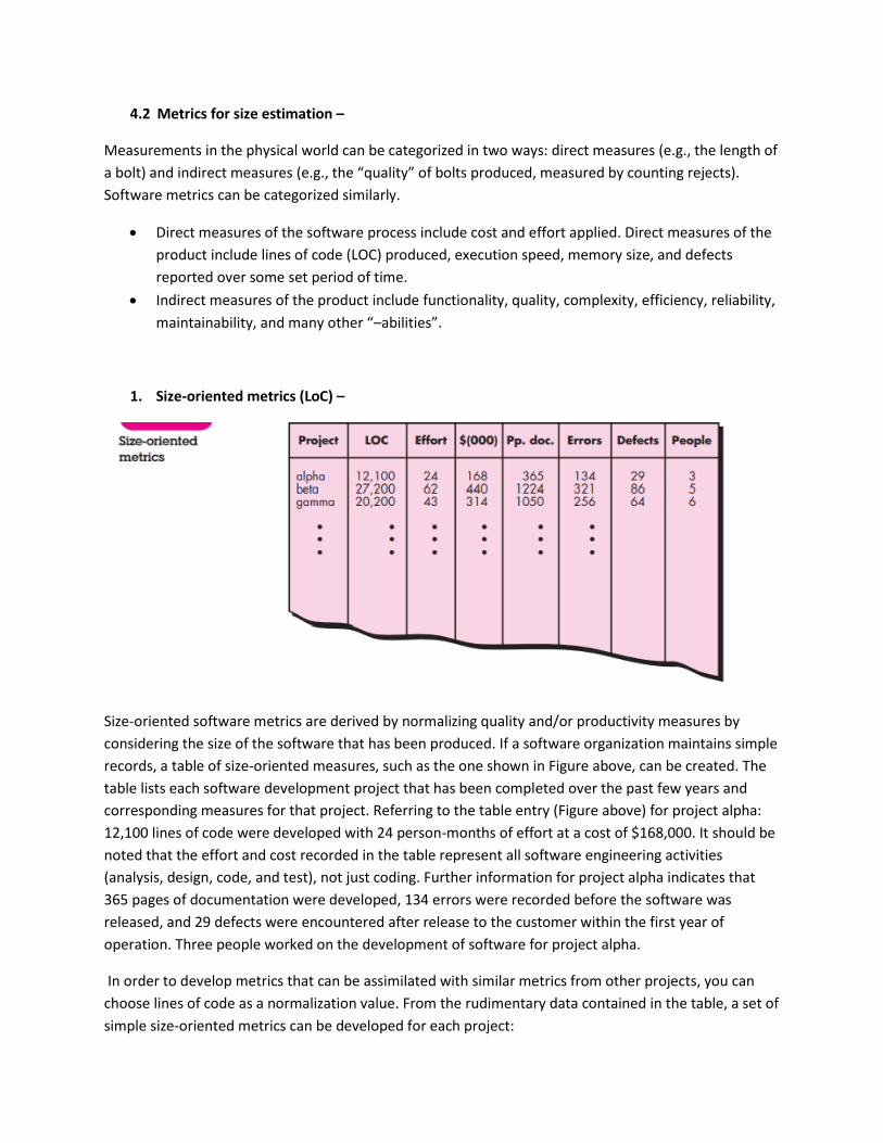
Size-oriented software metrics are derived by normalizing quality and/or productivity measures by

considering the size of the software that has been produced. If a software organization maintains simple

records, a table of size-oriented measures, such as the one shown in Figure above, can be created. The

table lists each software development project that has been completed over the past few years and

corresponding measures for that project. Referring to the table entry (Figure above) for project alpha:

12,100 lines of code were developed with 24 person-months of effort at a cost of $168,000. It should be

noted that the effort and cost recorded in the table represent all software engineering activities

(analysis, design, code, and test), not just coding. Further information for project alpha indicates that

365 pages of documentation were developed, 134 errors were recorded before the software was

released, and 29 defects were encountered after release to the customer within the first year of

operation. Three people worked on the development of software for project alpha.

In order to develop metrics that can be assimilated with similar metrics from other projects, you can

choose lines of code as a normalization value. From the rudimentary data contained in the table, a set of

simple size-oriented metrics can be developed for each project:

• Errors per KLOC (thousand lines of code)

• Defects per KLOC

• $ per KLOC

• Pages of documentation per KLOC

In addition, other interesting metrics can be computed:

• Errors per person-month

• KLOC per person-month

• $ per page of documentation

Size-oriented metrics are not universally accepted as the best way to measure the software process.

2. Function-oriented metrics (Function points) –

Function-oriented software metrics use a measure of the functionality delivered by the application as a

normalization value. The most widely used function-oriented metric is the function point (FP).

Computation of the function point is based on characteristics of the software’s information domain and

complexity.

The function point (FP) metric can be used effectively as a means for measuring the functionality

delivered by a system.Using historical data, the FP metric can then be used to

(1) estimate the cost or effort required to design, code, and test the software;

(2) predict the number of errors that will be encountered during testing; and

(3) forecast the number of components and/or the number of projected source lines in the

implemented system.

Function points are derived using an empirical relationship based on countable (direct) measures of

software’s information domain and qualitative assessments of software complexity. Information domain

values are defined in the following manner:

Number of external inputs (EIs). Each external input originates from a user or is transmitted from

another application and provides distinct application-oriented data or control information. Inputs are

often used to update internal logical files (ILFs). Inputs should be distinguished from inquiries, which are

counted separately.

Number of external outputs (EOs). Each external output is derived data within the application that

provides information to the user. In this context external output refers to reports, screens, error

messages, etc. Individual data items within a report are not counted separately.

Number of external inquiries (EQs). An external inquiry is defined as an online input that results in the

generation of some immediate software response in the form of an online output (often retrieved from

an ILF).

Number of internal logical files (ILFs). Each internal logical file is a logical grouping of data that resides

within the application’s boundary and is maintained via external inputs.

Number of external interface files (EIFs). Each external interface file is a logical grouping of data that

resides external to the application but provides information that may be of use to the application.

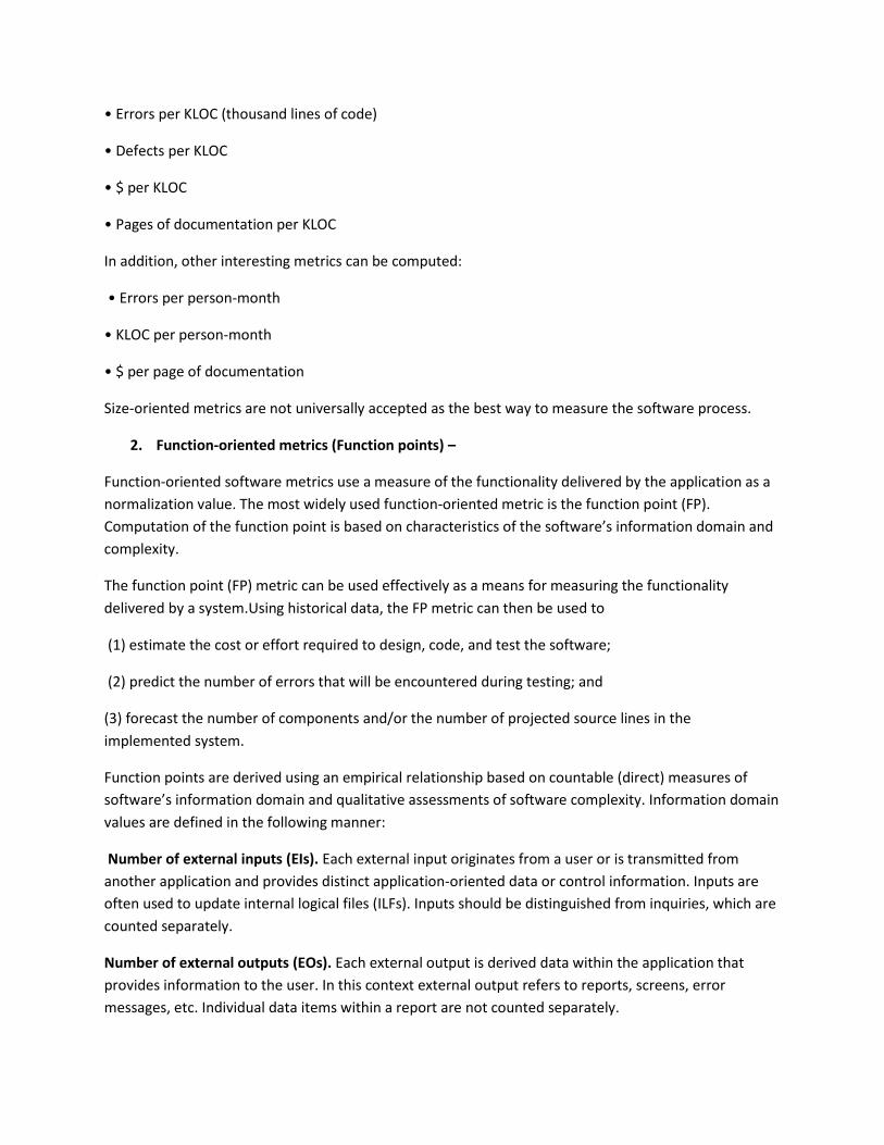
Once these data have been collected, the table in Figure below is completed and a complexity value is

associated with each count.

Organizations that use function point methods develop criteria for determining whether a particular

entry is simple, average, or complex.

To compute function points (FP), the following relationship is used:

FP =count total* [0.65 + 0.01 *Σ(Fi )]

where count total is the sum of all FP entries obtained from Figure above.

The Fi (i 1 to 14) are value adjustment factors (VAF) based on responses to the following sample

questions.

1. Does the system require reliable backup and recovery?

2. Are specialized data communications required to transfer information to or from the application?

3. Are there distributed processing functions?

4. Is performance critical?

5. Will the system run in an existing, heavily utilized operational environment?

Each of these questions is answered using a scale that ranges from 0 (not important or applicable) to 5

(absolutely essential). The constant values in Equation above and the weighting factors that are applied

to information domain counts are determined empirically.

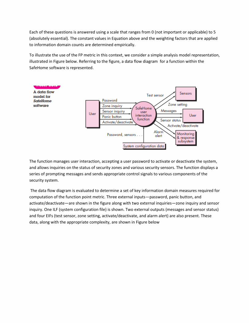
To illustrate the use of the FP metric in this context, we consider a simple analysis model representation,

illustrated in Figure below. Referring to the figure, a data flow diagram for a function within the

SafeHome software is represented.

The function manages user interaction, accepting a user password to activate or deactivate the system,

and allows inquiries on the status of security zones and various security sensors. The function displays a

series of prompting messages and sends appropriate control signals to various components of the

security system.

The data flow diagram is evaluated to determine a set of key information domain measures required for

computation of the function point metric. Three external inputs—password, panic button, and

activate/deactivate—are shown in the figure along with two external inquiries—zone inquiry and sensor

inquiry. One ILF (system configuration file) is shown. Two external outputs (messages and sensor status)

and four EIFs (test sensor, zone setting, activate/deactivate, and alarm alert) are also present. These

data, along with the appropriate complexity, are shown in Figure below

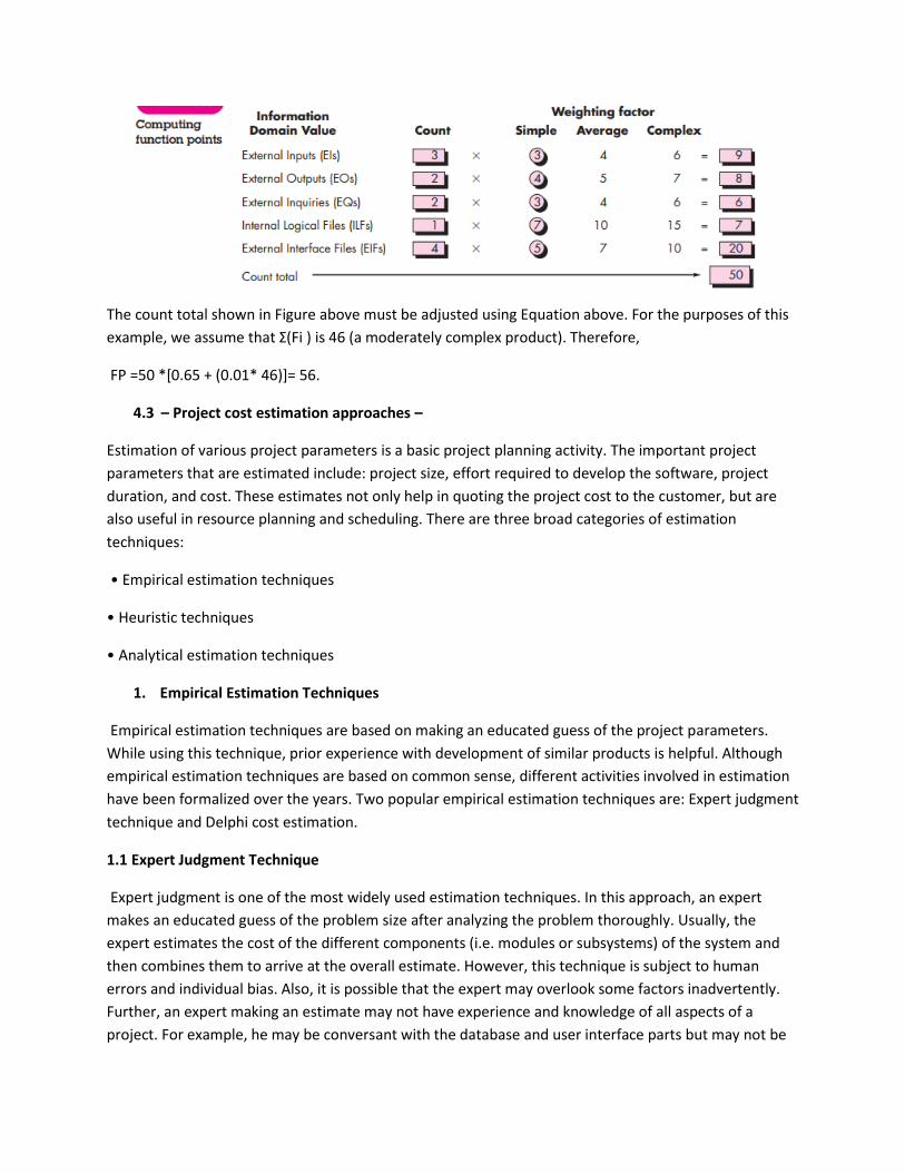
The count total shown in Figure above must be adjusted using Equation above. For the purposes of this

example, we assume that Σ(Fi ) is 46 (a moderately complex product). Therefore,

FP =50 *[0.65 + (0.01* 46)]= 56.

4.3 – Project cost estimation approaches –

Estimation of various project parameters is a basic project planning activity. The important project

parameters that are estimated include: project size, effort required to develop the software, project

duration, and cost. These estimates not only help in quoting the project cost to the customer, but are

also useful in resource planning and scheduling. There are three broad categories of estimation

techniques:

• Empirical estimation techniques

• Heuristic techniques

• Analytical estimation techniques

1. Empirical Estimation Techniques

Empirical estimation techniques are based on making an educated guess of the project parameters.

While using this technique, prior experience with development of similar products is helpful. Although

empirical estimation techniques are based on common sense, different activities involved in estimation

have been formalized over the years. Two popular empirical estimation techniques are: Expert judgment

technique and Delphi cost estimation.

1.1 Expert Judgment Technique

Expert judgment is one of the most widely used estimation techniques. In this approach, an expert

makes an educated guess of the problem size after analyzing the problem thoroughly. Usually, the

expert estimates the cost of the different components (i.e. modules or subsystems) of the system and

then combines them to arrive at the overall estimate. However, this technique is subject to human

errors and individual bias. Also, it is possible that the expert may overlook some factors inadvertently.

Further, an expert making an estimate may not have experience and knowledge of all aspects of a

project. For example, he may be conversant with the database and user interface parts but may not be

very knowledgeable about the computer communication part. A more refined form of expert judgment

is the estimation made by group of experts. Estimation by a group of experts minimizes factors such as

individual oversight, lack of familiarity with a particular aspect of a project, personal bias, and the desire

to win contract through overly optimistic estimates. However, the estimate made by a group of experts

may still exhibit bias on issues where the entire group of experts may be biased due to reasons such as

political considerations. Also, the decision made by the group may be dominated by overly assertive

members.

1.2 - Delphi cost estimation

Delphi cost estimation approach tries to overcome some of the shortcomings of the expert

judgment approach. Delphi estimation is carried out by a team comprising of a group of experts

and a coordinator. In this approach, the coordinator provides each estimator with a copy of the

software requirements specification (SRS) document and a form for recording his cost estimate.

Estimators complete their individual estimates anonymously and submit to the coordinator. In

their estimates, the estimators mention any unusual characteristic of the product which has

influenced his estimation. The coordinator prepares and distributes the summary of the

responses of all the estimators, and includes any unusual rationale noted by any of the

estimators. Based on this summary, the estimators re-estimate. This process is iterated for

several rounds. However, no discussion among the estimators is allowed during the entire

estimation process. The idea behind this is that if any discussion is allowed among the

estimators, then many estimators may easily get influenced by the rationale of an estimator

who may be more experienced or senior. After the completion of several iterations of

estimations, the coordinator takes the responsibility of compiling the results and preparing the

final estimate.

2. Heuristic Techniques

Heuristic techniques assume that the relationships among the different project parameters can

be modeled using suitable mathematical expressions. Once the basic (independent) parameters

are known, the other (dependent) parameters can be easily determined by substituting the

value of the basic parameters in the mathematical expression. Different heuristic estimation

models can be divided into the following two classes: single variable model and the multi

variable model.

Single variable estimation models provide a means to estimate the desired characteristics of a

problem, using some previously estimated basic (independent) characteristic of the software

product such as its size. A single variable estimation model takes the following form:

Estimated Parameter = c1 * ed 1

In the above expression, e is the characteristic of the software which has already been

estimated (independent variable). Estimated Parameter is the dependent parameter to be

estimated. The dependent parameter to be estimated could be effort, project duration, staff

size, etc. c1 and d1 are constants. The values of the constants c1 and d1 are usually determined

using data collected from past projects (historical data). The basic COCOMO model is an

example of single variable cost estimation model.

A multivariable cost estimation model takes the following form:

Estimated Resource = c1*e1 d1 + c2*e2 d2 + ...

Where e1, e2, … are the basic (independent) characteristics of the software already estimated,

and c1, c2, d1, d2, … are constants. Multivariable estimation models are expected to give more

accurate estimates compared to the single variable models, since a project parameter is

typically influenced by several independent parameters. The independent parameters influence

the dependent parameter to different extents. This is modeled by the constants c1, c2, d1, d2, …

. Values of these constants are usually determined from historical data. The intermediate

COCOMO model can be considered to be an example of a multivariable estimation model.

3. Analytical Estimation Techniques

Analytical estimation techniques derive the required results starting with basic assumptions

regarding the project. Thus, unlike empirical and heuristic techniques, analytical techniques do

have scientific basis. Halstead’s software science is an example of an analytical technique.

Halstead’s software science can be used to derive some interesting results starting with a few

simple assumptions. Halstead’s software science is especially useful for estimating software

maintenance efforts. In fact, it outperforms both empirical and heuristic techniques when used

for predicting software maintenance efforts.

3.1 Halstead’s Software Science –

An Analytical Technique Halstead’s software science is an analytical technique to measure size,

development effort, and development cost of software products. Halstead used a few primitive

program parameters to develop the expressions for over all program length, potential minimum

value, actual volume, effort, and development time.

For a given program, let: ƒ

η1 be the number of unique operators used in the program,

ƒ η2 be the number of unique operands used in the program,

ƒ N1 be the total number of operators used in the program, ƒ

N2 be the total number of operands used in the program.

a. Length and Vocabulary

The length of a program as defined by Halstead, quantifies total usage of all operators and

operands in the program. Thus, length N = N1 +N2. Halstead’s definition of the length of the

program as the total number of operators and operands roughly agrees with the intuitive

notation of the program length as the total number of tokens used in the program. The program

vocabulary is the number of unique operators and operands used in the program. Thus,

program vocabulary η = η1 + η2.

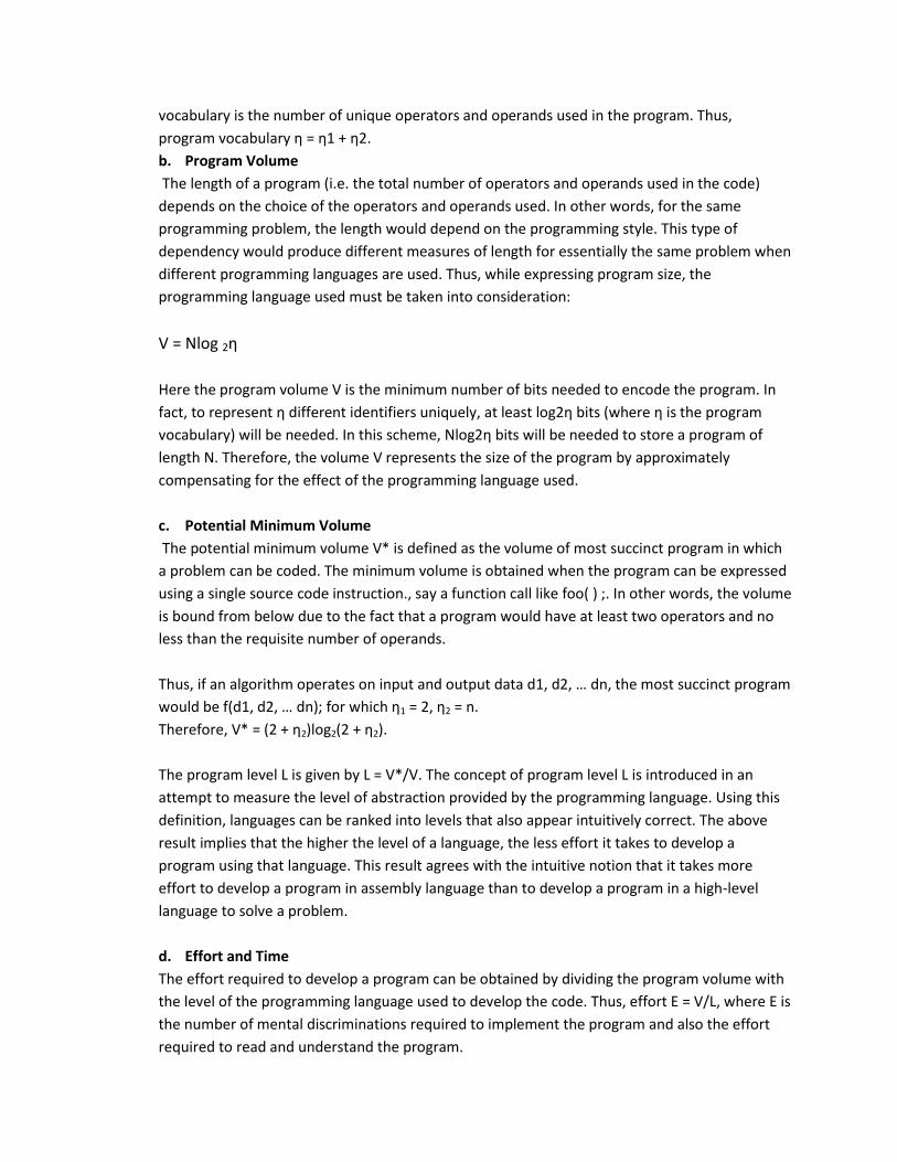
b. Program Volume

The length of a program (i.e. the total number of operators and operands used in the code)

depends on the choice of the operators and operands used. In other words, for the same

programming problem, the length would depend on the programming style. This type of

dependency would produce different measures of length for essentially the same problem when

different programming languages are used. Thus, while expressing program size, the

programming language used must be taken into consideration:

V = Nlog 2η

Here the program volume V is the minimum number of bits needed to encode the program. In

fact, to represent η different identifiers uniquely, at least log2η bits (where η is the program

vocabulary) will be needed. In this scheme, Nlog2η bits will be needed to store a program of

length N. Therefore, the volume V represents the size of the program by approximately

compensating for the effect of the programming language used.

c. Potential Minimum Volume

The potential minimum volume V* is defined as the volume of most succinct program in which

a problem can be coded. The minimum volume is obtained when the program can be expressed

using a single source code instruction., say a function call like foo( ) ;. In other words, the volume

is bound from below due to the fact that a program would have at least two operators and no

less than the requisite number of operands.

Thus, if an algorithm operates on input and output data d1, d2, … dn, the most succinct program

would be f(d1, d2, … dn); for which η1 = 2, η2 = n.

Therefore, V* = (2 + η2)log2(2 + η2).

The program level L is given by L = V*/V. The concept of program level L is introduced in an

attempt to measure the level of abstraction provided by the programming language. Using this

definition, languages can be ranked into levels that also appear intuitively correct. The above

result implies that the higher the level of a language, the less effort it takes to develop a

program using that language. This result agrees with the intuitive notion that it takes more

effort to develop a program in assembly language than to develop a program in a high-level

language to solve a problem.

d. Effort and Time

The effort required to develop a program can be obtained by dividing the program volume with

the level of the programming language used to develop the code. Thus, effort E = V/L, where E is

the number of mental discriminations required to implement the program and also the effort

required to read and understand the program.

Thus, the programming effort E = V²/V* (since L = V*/V) varies as the square of the volume.

Experience shows that E is well correlated to the effort needed for maintenance of an existing

program.

The programmer’s time T = E/S, where S the speed of mental discriminations. The value of S has

been empirically developed from psychological reasoning, and its recommended value for

programming applications is 18.

COCOMO Model

Boehm proposed COCOMO (Constructive Cost Estimation Model) in 1981.COCOMO is one of

the most generally used software estimation models in the world. COCOMO predicts the efforts and schedule of a software product based on the size of the software.

The necessary steps in this model are:

1. Get an initial estimate of the development effort from evaluation of thousands of

delivered lines of source code (KDLOC).

2. Determine a set of 15 multiplying factors from various attributes of the project.

3. Calculate the effort estimate by multiplying the initial estimate with all the

multiplying factors i.e., multiply the values in step1 and step2.

The initial estimate (also called nominal estimate) is determined by an equation of the form

used in the static single variable models, using KDLOC as the measure of the size. To

determine the initial effort Ei in person-months the equation used is of the type is shown below

Ei=a*(KDLOC)b

The value of the constant a and b are depends on the project type.

In COCOMO, projects are categorized into three types:

1. Organic

2. Semidetached

3. Embedded

1.Organic: A development project can be treated of the organic type, if the project deals

with developing a well-understood application program, the size of the development team is

reasonably small, and the team members are experienced in developing similar methods of

projects. Examples of this type of projects are simple business systems, simple inventory management systems, and data processing systems.

2. Semidetached: A development project can be treated with semidetached type if the

development consists of a mixture of experienced and inexperienced staff. Team members

may have finite experience in related systems but may be unfamiliar with some aspects of

the order being developed. Example of Semidetached system includes developing a

new operating system (OS), a Database Management System (DBMS), and complex inventory management system.

3. Embedded: A development project is treated to be of an embedded type, if the software

being developed is strongly coupled to complex hardware, or if the stringent regulations on the operational method exist. For Example: ATM, Air Traffic control.

For three product categories, Bohem provides a different set of expression to predict effort

(in a unit of person month)and development time from the size of estimation in KLOC(Kilo

Line of code) efforts estimation takes into account the productivity loss due to holidays,

weekly off, coffee breaks, etc.

According to Boehm, software cost estimation should be done through three stages:

1. Basic Model

2. Intermediate Model

3. Detailed Model

1. Basic COCOMO Model: The basic COCOMO model provide an accurate size of the project parameters. The following expressions give the basic COCOMO estimation model:

Effort=a1*(KLOC) a2 PM Tdev=b1*(efforts)b2 Months

Where

KLOC is the estimated size of the software product indicate in Kilo Lines of Code,

a1,a2,b1,b2 are constants for each group of software products,

Tdev is the estimated time to develop the software, expressed in months,

Effort is the total effort required to develop the software product, expressed in person months (PMs).

Estimation of development effort

For the three classes of software products, the formulas for estimating the effort based on the code size are shown below:

Organic: Effort = 2.4(KLOC) 1.05 PM

Semi-detached: Effort = 3.0(KLOC) 1.12 PM

Embedded: Effort = 3.6(KLOC) 1.20 PM

Estimation of development time

For the three classes of software products, the formulas for estimating the development time based on the effort are given below:

Organic: Tdev = 2.5(Effort) 0.38 Months

Semi-detached: Tdev = 2.5(Effort) 0.35 Months

Embedded: Tdev = 2.5(Effort) 0.32 Months

Example1: Suppose a project was estimated to be 400 KLOC. Calculate the effort and development time for each of the three model i.e., organic, semi-detached & embedded.

Solution: The basic COCOMO equation takes the form:

Effort=a1*(KLOC) a2 PM

Tdev=b1*(efforts)b2 Months Estimated Size of project= 400 KLOC

(i)Organic Mode

E = 2.4 * (400)1.05 = 1295.31 PM D = 2.5 * (1295.31)0.38=38.07 PM

(ii)Semidetached Mode

E = 3.0 * (400)1.12=2462.79 PM D = 2.5 * (2462.79)0.35=38.45 PM

(iii) Embedded Mode

E = 3.6 * (400)1.20 = 4772.81 PM D = 2.5 * (4772.8)0.32 = 38 PM

Example2: A project size of 200 KLOC is to be developed. Software development team has

average experience on similar type of projects. The project schedule is not very tight. Calculate the Effort, development time, average staff size, and productivity of the project.

Solution: The semidetached mode is the most appropriate mode, keeping in view the size, schedule and experience of development time.

Hence E=3.0(200)1.12=1133.12PM D=2.5(1133.12)0.35=29.3PM

P = 176 LOC/PM

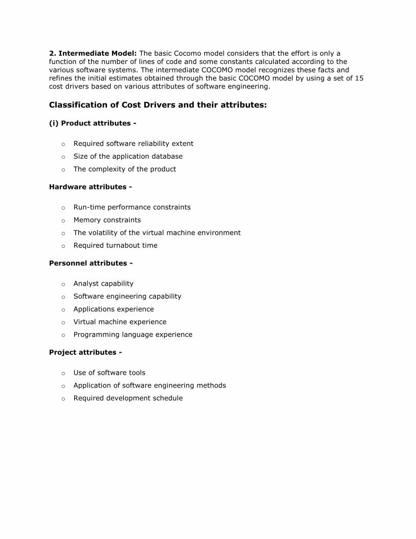
2. Intermediate Model: The basic Cocomo model considers that the effort is only a

function of the number of lines of code and some constants calculated according to the

various software systems. The intermediate COCOMO model recognizes these facts and

refines the initial estimates obtained through the basic COCOMO model by using a set of 15 cost drivers based on various attributes of software engineering.

Classification of Cost Drivers and their attributes:

(i) Product attributes -

o Required software reliability extent

o Size of the application database

o The complexity of the product

Hardware attributes -

o Run-time performance constraints

o Memory constraints

o The volatility of the virtual machine environment

o Required turnabout time

Personnel attributes -

o Analyst capability

o Software engineering capability

o Applications experience

o Virtual machine experience

o Programming language experience

Project attributes -

o Use of software tools

o Application of software engineering methods

o Required development schedule

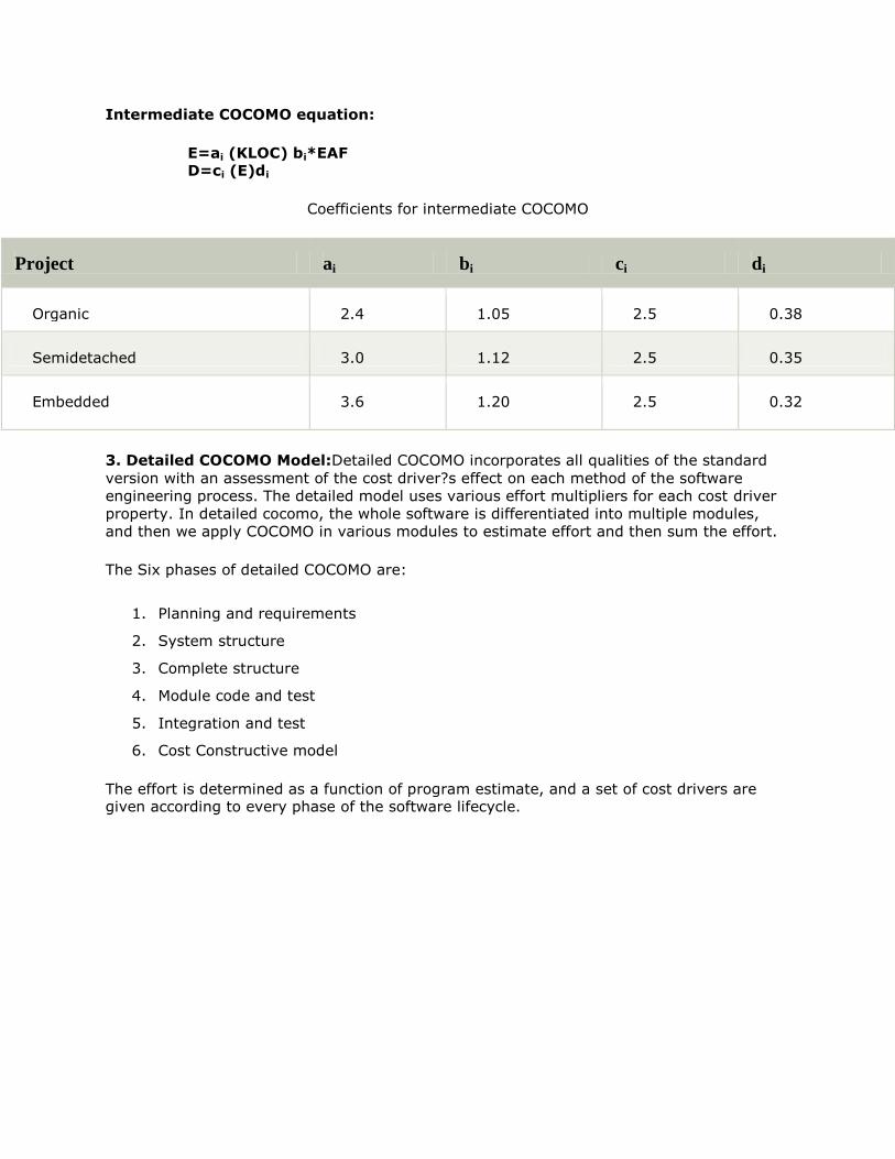
Intermediate COCOMO equation:

E=ai (KLOC) bi*EAF D=ci (E)di

Coefficients for intermediate COCOMO

Project ai bi ci di

Organic 2.4 1.05 2.5 0.38

Semidetached 3.0 1.12 2.5 0.35

Embedded 3.6 1.20 2.5 0.32

3. Detailed COCOMO Model:Detailed COCOMO incorporates all qualities of the standard

version with an assessment of the cost driver?s effect on each method of the software

engineering process. The detailed model uses various effort multipliers for each cost driver

property. In detailed cocomo, the whole software is differentiated into multiple modules,

and then we apply COCOMO in various modules to estimate effort and then sum the effort.

The Six phases of detailed COCOMO are:

1. Planning and requirements

2. System structure

3. Complete structure

4. Module code and test

5. Integration and test

6. Cost Constructive model

The effort is determined as a function of program estimate, and a set of cost drivers are given according to every phase of the software lifecycle.

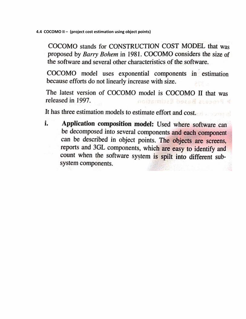
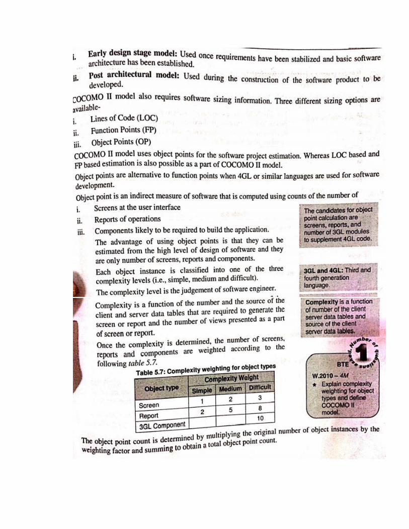
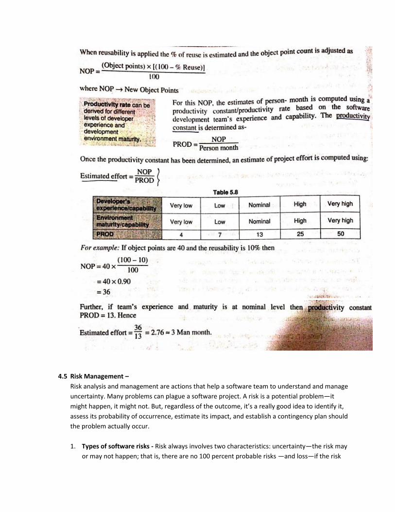
4.4 COCOMO II – (project cost estimation using object points)

4.5 Risk Management –

Risk analysis and management are actions that help a software team to understand and manage

uncertainty. Many problems can plague a software project. A risk is a potential problem—it

might happen, it might not. But, regardless of the outcome, it’s a really good idea to identify it,

assess its probability of occurrence, estimate its impact, and establish a contingency plan should

the problem actually occur.

1. Types of software risks - Risk always involves two characteristics: uncertainty—the risk may

or may not happen; that is, there are no 100 percent probable risks —and loss—if the risk

becomes a reality, unwanted consequences or losses will occur. When risks are analyzed, it

is important to quantify the level of uncertainty and the degree of loss associated with each

risk.

To accomplish this, different categories of risks are considered.

a. Project risks threaten the project plan. That is, if project risks become real, it is

likely that the project schedule will slip and that costs will increase. Project risks

identify potential budgetary, schedule, personnel (staffing and organization),

resource, stakeholder, and requirements problems and their impact on a

software project. Project complexity, size, and the degree of structural

uncertainty were also defined as project (and estimation) risk factors.

b. Technical risks threaten the quality and timeliness of the software to be

produced. If a technical risk becomes a reality, implementation may become

difficult or impossible. Technical risks identify potential design, implementation,

interface, verification, and maintenance problems. In addition, specification

ambiguity, technical uncertainty, technical obsolescence, and “leading-edge”

technology are also risk factors. Technical risks occur because the problem is

harder to solve than you thought it would be.

c. Business risks threaten the viability of the software to be built and often

jeopardize the project or the product. Candidates for the top five business risks

are (1) building an excellent product or system that no one really wants (market

risk), (2) building a product that no longer fits into the overall business strategy

for the company (strategic risk), (3) building a product that the sales force

doesn’t understand how to sell (sales risk), (4) losing the support of senior

management due to a change in focus or a change in people (management risk),

and (5) losing budgetary or personnel commitment (budget risks).

It is extremely important to note that simple risk categorization won’t always work. Some risks are

simply unpredictable in advance. Another general categorization of risks has been proposed.

a. Known risks are those that can be uncovered after careful evaluation of

the project plan, the business and technical environment in which the

project is being developed, and other reliable information sources (e.g.,

unrealistic delivery date, lack of documented requirements or software

scope, poor development environment).

b. Predictable risks are extrapolated from past project experience (e.g.,

staff turnover, poor communication with the customer, dilution of staff

effort as ongoing maintenance requests are serviced). Unpredictable

risks are the joker in the deck. They can and do occur, but they are

extremely difficult to identify in advance.

2. Seven principles of risk management –

Seven principles that “provide a framework to accomplish effective risk management.” They are:

Maintain a global perspective—view software risks within the context of a system in which it is a

component and the business problem that it is intended to solve

Take a forward-looking view—think about the risks that may arise in the future (e.g., due to changes in

the software); establish contingency plans so that future events are manageable.

Encourage open communication—if someone states a potential risk, don’t discount it. If a risk is

proposed in an informal manner, consider it. Encourage all stakeholders and users to suggest risks at any

time.

Integrate—a consideration of risk must be integrated into the software process.

Emphasize a continuous process—the team must be vigilant throughout the software process,

modifying identified risks as more information is known and adding new ones as better insight is

achieved.

Develop a shared product vision—if all stakeholders share the same vision of the software, it is likely

that better risk identification and assessment will occur.

Encourage teamwork—the talents, skills, and knowledge of all stakeholders should be pooled when risk

management activities are conducted.

3. Risk Identification –

Risk identification is a systematic attempt to specify threats to the project plan (estimates, schedule,

resource loading, etc.). By identifying known and predictable risks, the project manager takes a first step

toward avoiding them when possible and controlling them when necessary.

There are two distinct types of risks for each of the categories: generic risks and product-specific risks.

Generic risks are a potential threat to every software project. Product-specific risks can be identified

only by those with a clear understanding of the technology, the people, and the environment that is

specific to the software that is to be built.

To identify product-specific risks, the project plan and the software statement of scope are examined,

and an answer to the following question is developed: “What special characteristics of this product may

threaten our project plan?” One method for identifying risks is to create a risk item checklist.

The checklist can be used for risk identification and focuses on some subset of known and predictable

risks in the following generic subcategories:

• Product size—risks associated with the overall size of the software to be built or modified.

• Business impact—risks associated with constraints imposed by management or the marketplace.

•Stakeholder characteristics—risks associated with the sophistication of the stakeholders and the

developer’s ability to communicate with stakeholders in a timely manner.

• Process definition—risks associated with the degree to which the software process has been defined

and is followed by the development organization.

• Development environment—risks associated with the availability and quality of the tools to be used to

build the product.

• Technology to be built—risks associated with the complexity of the system to be built and the

“newness” of the technology that is packaged by the system.

• Staff size and experience—risks associated with the overall technical and project experience of the

software engineers who will do the work.

The risk item checklist can be organized in different ways. Questions relevant to each of the topics can

be answered for each software project. The answers to these questions allow you to estimate the

impact of risk.

4. Risk Assessment –

The following questions have been derived from risk data obtained by surveying experienced software

project managers in different parts of the world . The questions are ordered by their relative importance

to the success of a project.

1. Have top software and customer managers formally committed to support the project?

2. Are end users enthusiastically committed to the project and the system/ product to be built?

3. Are requirements fully understood by the software engineering team and its customers?

4. Have customers been involved fully in the definition of requirements?

5. Do end users have realistic expectations?

6. Is the project scope stable?

7. Does the software engineering team have the right mix of skills?

8. Are project requirements stable?

9. Does the project team have experience with the technology to be implemented?

10. Is the number of people on the project team adequate to do the job?

11. Do all customer/user constituencies agree on the importance of the project and on the

requirements for the system/product to be built?

If any one of these questions is answered negatively, mitigation, monitoring, and management steps

should be instituted without fail. The degree to which the project is at risk is directly proportional to the

number of negative responses to these questions.

5. Risk Mitigation, Monitoring, and Management (RMMM) –

All of the risk analysis activities presented to this point have a single goal—to assist the project team in

developing a strategy for dealing with risk. An effective strategy must consider three issues: risk

avoidance, risk monitoring, and risk management and contingency planning. If a software team adopts a

proactive approach to risk, avoidance is always the best strategy. This is achieved by developing a plan

for risk mitigation.

For example, assume that high staff turnover is noted as a project risk r1. Based on past history and

management intuition, the likelihood l1 of high turnover is estimated to be 0.70 (70 percent, rather

high) and the impact x1 is projected as critical. That is, high turnover will have a critical impact on project

cost and schedule.

To mitigate this risk, you would develop a strategy for reducing turnover. Among the possible steps to

be taken are:

• Meet with current staff to determine causes for turnover (e.g., poor working conditions, low pay,

competitive job market).

• Mitigate those causes that are under your control before the project starts.

• Once the project commences, assume turnover will occur and develop techniques to ensure

continuity when people leave.

• Organize project teams so that information about each development activity is widely dispersed.

•Define work product standards and establish mechanisms to be sure that all models and documents

are developed in a timely manner.

• Conduct peer reviews of all work (so that more than one person is “up to speed”).

• Assign a backup staff member for every critical technologist.

As the project proceeds, risk-monitoring activities commence. The project manager monitors factors

that may provide an indication of whether the risk is becoming more or less likely. In the case of high

staff turnover, the general attitude of team members based on project pressures, the degree to which

the team has jelled, interpersonal relationships among team members, potential problems with

compensation and benefits, and the availability of jobs within the company and outside it are all

monitored.

Risk management and contingency planning assumes that mitigation efforts have failed and that the

risk has become a reality. Continuing the example, the project is well under way and a number of people

announce that they will be leaving. If the mitigation strategy has been followed, backup is available,

information is documented, and knowledge has been dispersed across the team. In addition, you can

temporarily refocus resources (and readjust the project schedule) to those functions that are fully

staffed, enabling newcomers who must be added to the team to “get up to speed.” Those individuals

who are leaving are asked to stop all work and spend their last weeks in “knowledge transfer mode.”

This might include video-based knowledge capture, the development of “commentary documents or

Wikis,” and/or meeting with other team members who will remain on the project

6. The RMMM plan –

A risk management strategy can be included in the software project plan, or the risk management steps

can be organized into a separate risk mitigation, monitoring, and management plan (RMMM). The

RMMM plan documents all work performed as part of risk analysis and is used by the project manager

as part of the overall project plan. Some software teams do not develop a formal RMMM document.

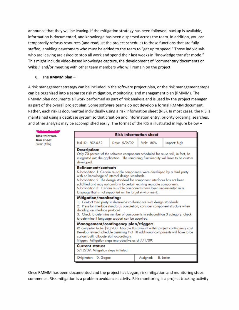
Rather, each risk is documented individually using a risk information sheet (RIS). In most cases, the RIS is

maintained using a database system so that creation and information entry, priority ordering, searches,

and other analysis may be accomplished easily. The format of the RIS is illustrated in Figure below –

Once RMMM has been documented and the project has begun, risk mitigation and monitoring steps

commence. Risk mitigation is a problem avoidance activity. Risk monitoring is a project tracking activity

with three primary objectives: (1) to assess whether predicted risks do, in fact, occur; (2) to ensure that

risk aversion steps defined for the risk are being properly applied; and (3) to collect information that can

be used for future risk analysis. In many cases, the problems that occur during a project can be traced to

more than one risk. Another job of risk monitoring is to attempt to allocate origin [what risk(s) caused

which problems throughout the project].