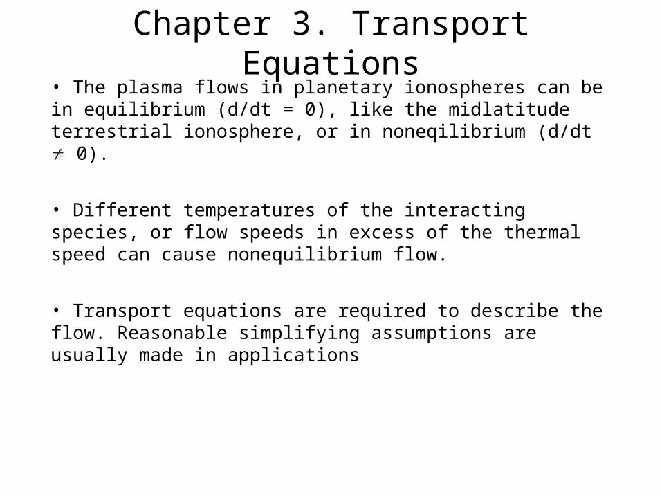
Chapter 3. Transport Equations• The plasma flows in planetary ionospheres can be in equilibrium (d/dt = 0), like the midlatitude terrestrial ionosphere, or in noneqilibrium (d/dt 0).

• Different temperatures of the interacting species, or flow speeds in excess of the thermal speed can cause nonequilibrium flow.

• Transport equations are required to describe the flow. Reasonable simplifying assumptions are usually made in applications

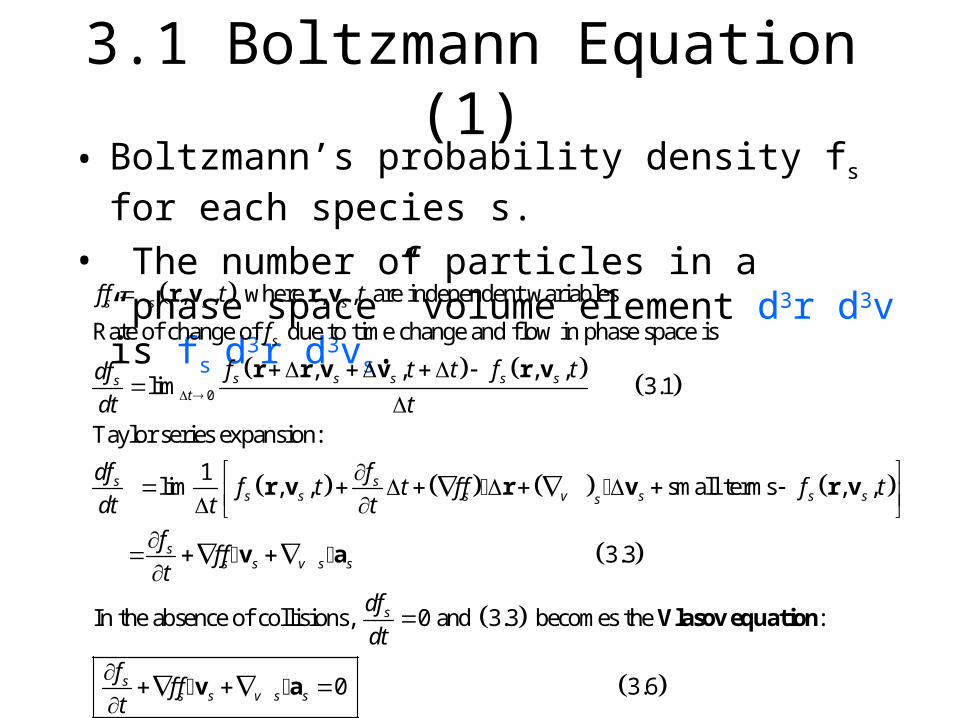
3.1 Boltzmann Equation (1)• Boltzmann’s probability density fs for each species s.

• The number of particles in a “phase space” volume element d3r d3v is fs d3r d3vs.

0

, , where , , are independent wariables

Rate of change of due to time change and flow in phase space is

, , , ,lim 3.1

Taylor series expansion:

1lim

s s s s

s

s s s s sst

ss

f f t t

f

f t t f tdf

dt t

dff

dt t

r v r v

r r v v r v

r

, , small terms , ,

3.3

In the absence of collisions, 0 and 3.3 becomes the :

0 3.6

ss s v s s ss

ss s v s s

s

ss s v s s

ft t f f f t

t

ff f

tdf

dt

ff f

t

v r v r v

v a

Vlasov equation

v a

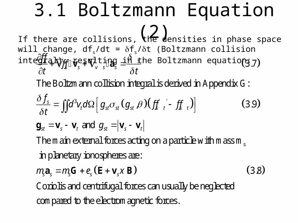
3.1 Boltzmann Equation (2)If there are collisions, the densities in phase space will change, dfs/dt = fs/t (Boltzmann collision integral), resulting in the Boltzmann equation:

3 ' '

3.7

The Boltzmann collision integral is derived in Appendix G:

, 3.9

and

The main external forces acting on a particle w

s ss s v s s

st st st st s t s t

st s t st s t

f ff f

t t

fd v d g g f f f f

tg

v a

g v v v v

sith mass m

in planetary ionospheres are:

3.8

Coriolis and centrifugal forces can usually be neglected

compared to the electromagnetic forces.

s s s s sm m e x a G E v B

3.2 Velocity Moments of Distribution Functions (1)

s

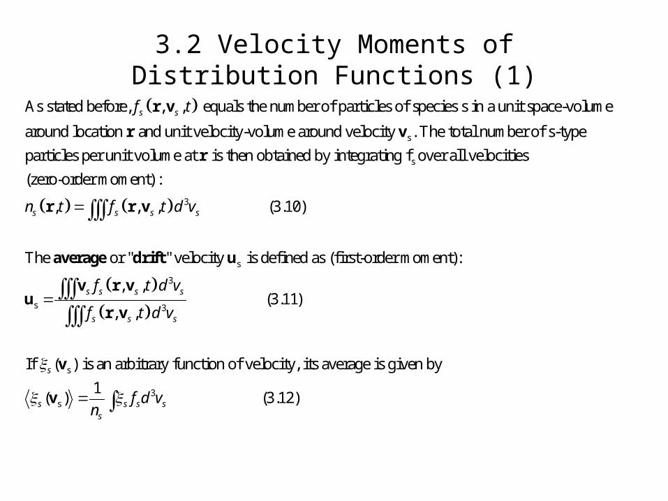
As stated before, , , equals the number of particles of species s in a unit space-volume

around location and unit velocity-volume around velocity . The total number of s-type

particles per uni

s sf tr v

r v

s

3

s

3

s

t volume at is then obtained by integrating f over all velocities

(zero-order moment) :

, , , (3.10)

The or " " velocity is defined as (first-order moment):

, ,

s s s s

s s s

n t f t d v

f t d

r

r r v

average drift u

v r vu

3

s

3s

(3.11), ,

If ( ) is an arbitrary function of velocity, its average is given by

1( ) (3.12)

s

s s s

s

s s s ss

v

f t d v

f d vn

r v

v

v

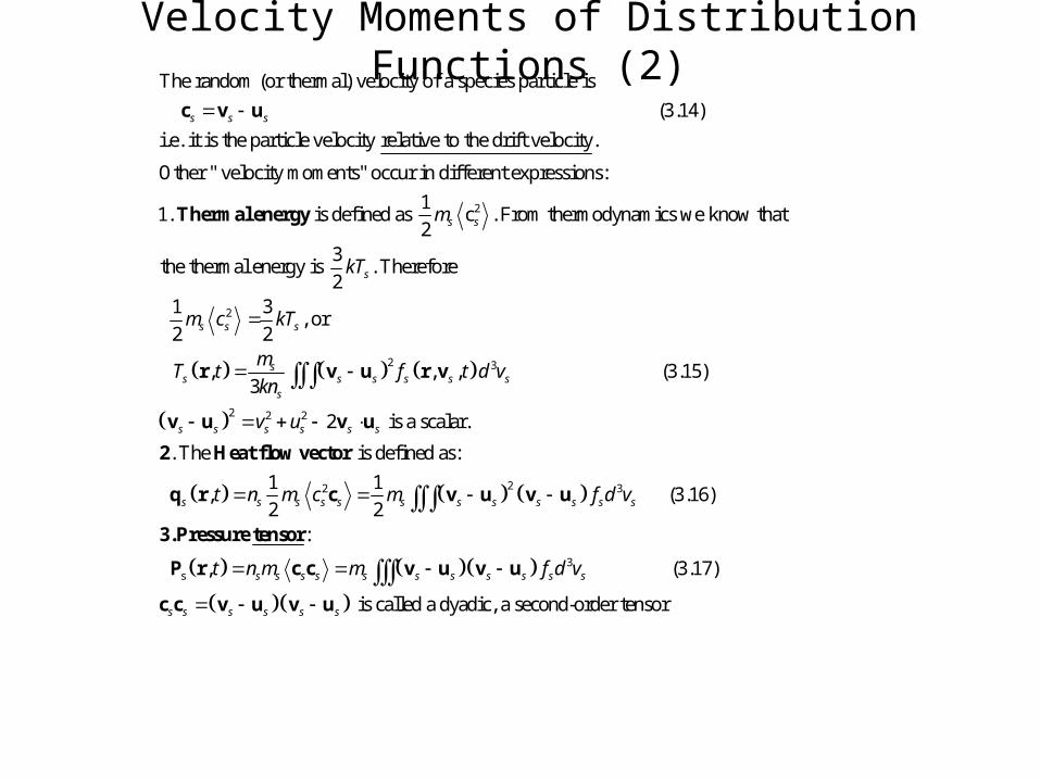
Velocity Moments of Distribution Functions (2)The random (or thermal) velocity of a species particle is

(3.14)

i.e. it is the particle velocity relative to the drift velocity.

Other " velocity moments" occur in different expressions:

1.

s s s c v u

Ther

2

2

2 3

2 2 2

1is defined as c . From thermodynamics we know that

23

the thermal energy is . Therefore2

1 3, or

2 2

, , , (3.15)3

2 is a scalar.

. Th

s s

s

s s s

ss s s s s s

s

s s s s s s

m

kT

m c kT

mT t f t d v

kn

v u

mal energy

r v u r v

v u v u

2

22 3

3s

e is defined as:

1 1, (3.16)

2 2:

, (3.17)

is called a dyadic, a second-order tensor

s s s s s s s s s s s s

s s s s s s s s s s s

s s s s s s

t n m c m f d v

t n m m f d v

Heat flow vector

q r c v u v u

3.Pressure tensor

P r c c v u v u

c c v u v u

Moments of Distribution Functions (3)

11 12 13

21 22 23

31 32 33 s

3

3

3

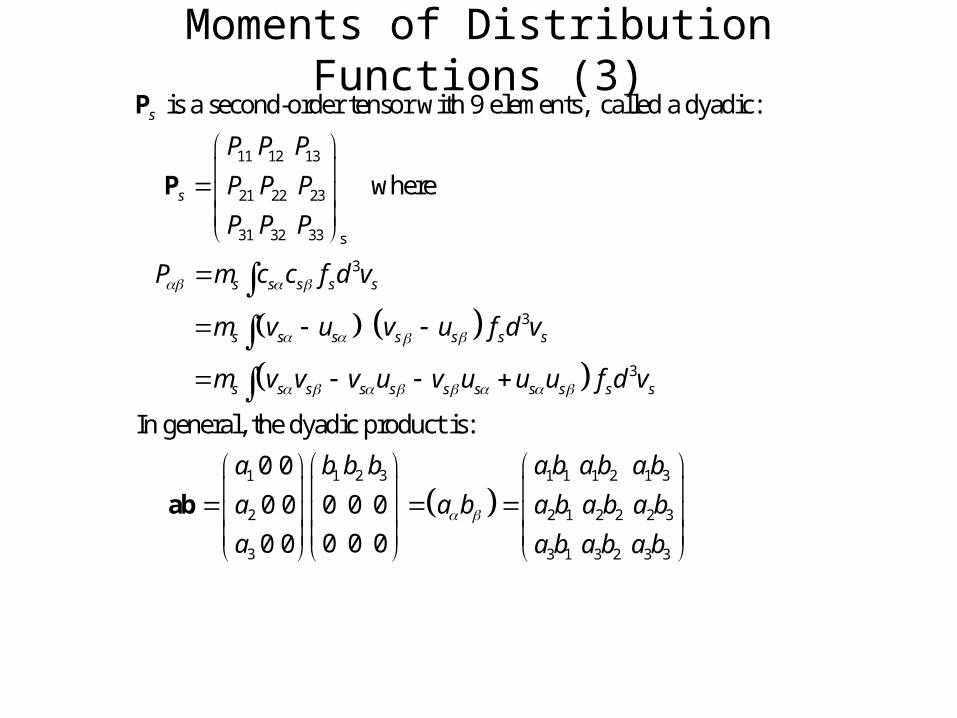
is a second-order tensor with 9 elements, called a dyadic:

where

In genera

s

s

s s s s s

s s s s s s s

s s s s s s s s s s s

P P P

P P P

P P P

P m c c f d v

m v u v u f d v

m v v v u v u u u f d v

P

P

1 2 3 1 1 1 2 1 31

2 2 1 2 2 2 3

3 3 1 3 2 3 3

l, the dyadic product is:

0 0

0 0 0 0 0

0 0 00 0

b b b a b a b a ba

a a b a b a b a b

a a b a b a b

ab

Moments of Distribution Functions (4)

s s

32 2 2 3 2 3 211 22 33

1

2

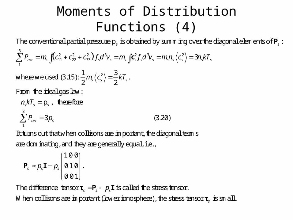
The conventional partial pressure p is obtained by summing over the diagonal elements of :

3

1 3where we used (3.15): .

2 2From the ideal

s s s s s s s s s s s s

s s s

P m c c c f d v m f d v m n c n kT

m c kT

P

c

3

1

gas law:

p , therefore

3 (3.20)

It turns out that when collisons are important, the diagonal terms

are dominating, and they are generally equal, i.e.,

1 0 0

0 1 0 .

0 0 1

The diffe

s s s

s

s s s

n kT

P p

p p

P I

rence tensor is called the stress tensor.

When collisons are important (lower ionosphere), the stress tensor is small.s s s

s

p τ P I

τ

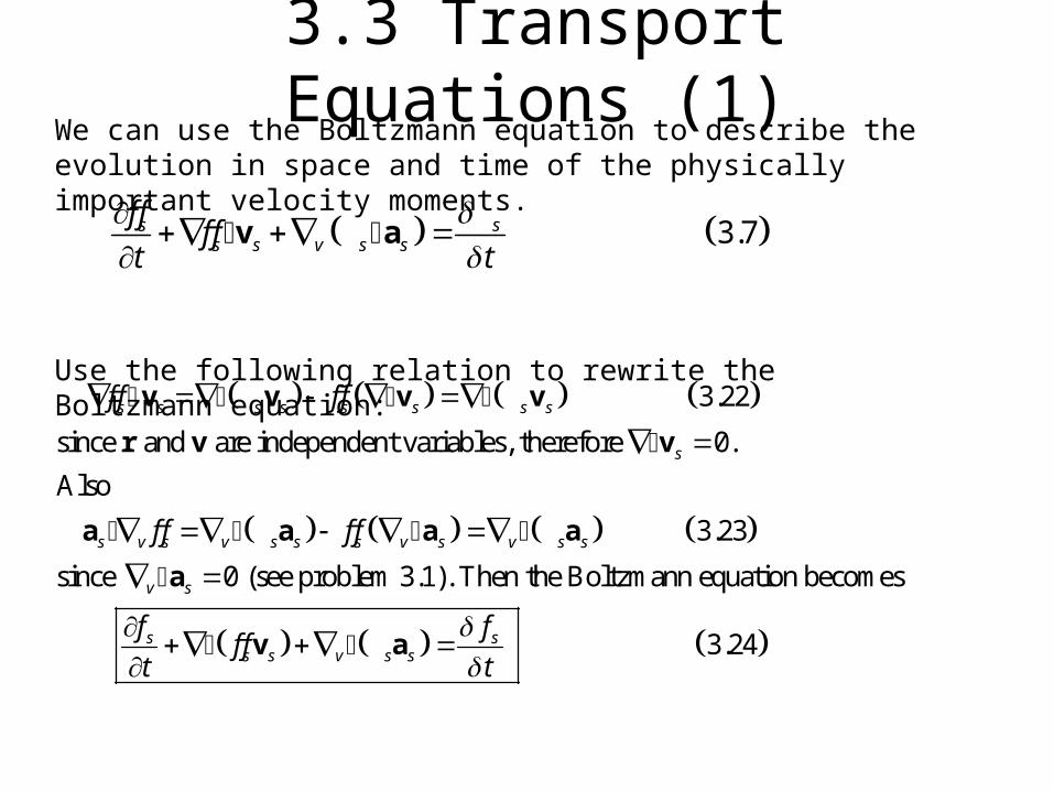
3.3 Transport Equations (1)We can use the Boltzmann equation to describe the evolution in space and time of the physically important velocity moments.

Use the following relation to rewrite the Boltzmann equation:

3.7s ss s v s s

f ff f

t t

v a

3.22

since and are independent variables, therefore 0.

Also

3.23

since 0 (see problem 3.1). Then the Boltzmann equation becomes

s s s s s s s s

s

s v s v s s s v s v s s

v s

s

f f f f

f f f f

f

v v v v

r v v

a a a a

a

3.24ss s v s s

ff f

t t

v a

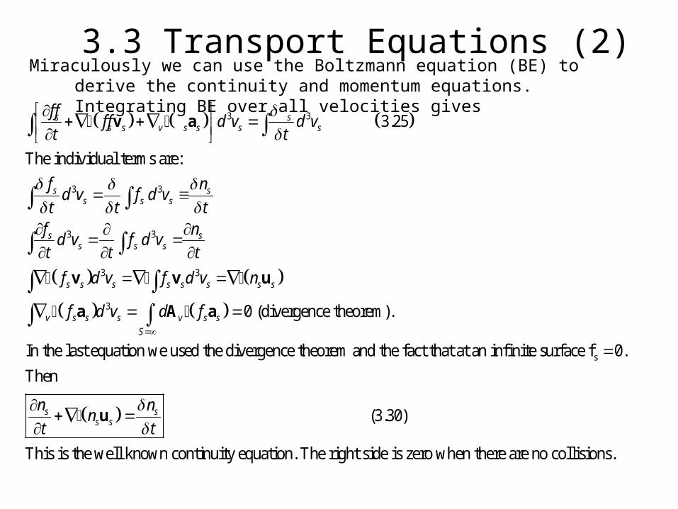
3.3 Transport Equations (2)Miraculously we can use the Boltzmann equation (BE) to derive the continuity and

momentum equations. Integrating BE over all velocities gives

3 3

3 3

3 3

3 3

3

3.25

The individual terms are:

0 (divergence theor

s ss s v s s s s

s ss s s

s ss s s

s s s s s s s s

v s s s v s s

S

f ff f d v d v

t t

f nd v f d v

t t tf nd v f d vt t t

f d v f d v n

f d v d f

v a

v v u

a A a

s

em).

In the last equation we used the divergence theorem and the fact that at an infinite surface f 0.

Then

(3.30)

This is the well known continuity equation. The right side is zero wh

s ss s

n nn

t t

u

en there are no collisions.

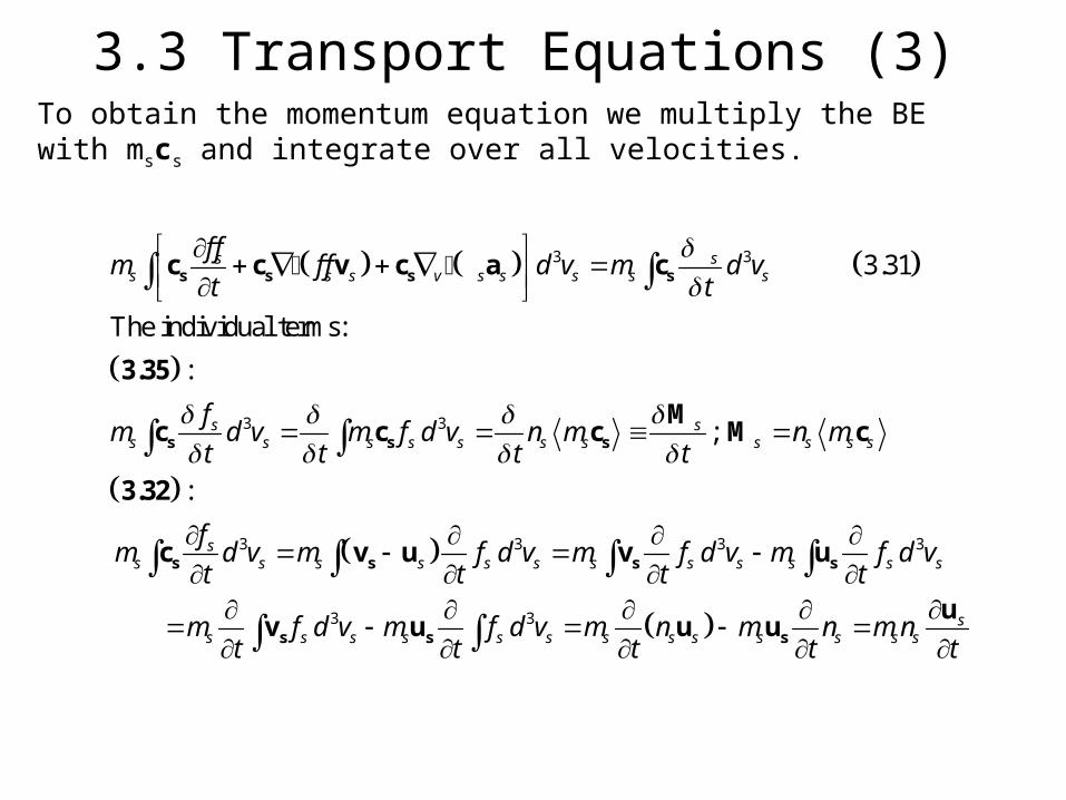
3.3 Transport Equations (3)To obtain the momentum equation we multiply the BE with mscs and integrate over all velocities.

3 3

3 3

3 3 3

3.31

The individual terms:

:

;

:

s ss s s v s s s s s

s ss s s s s s s s s s s

ss s s s s s s s s s

f fm f f d v m d v

t t

fm d v m f d v n m n m

t t t t

fm d v m f d v m f d v m f

t t t t

s s s s

s s s

s s s s

c c v c a c

3.35

Mc c c M c

3.32

c v u v u

3

3 3

s s

ss s s s s s s s s s s s s

d v

m f d v m f d v m n m n m nt t t t t

s s s

uv u u u

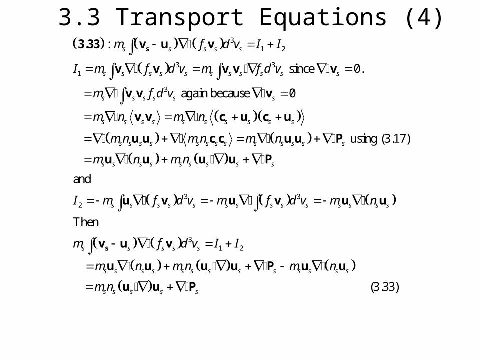
3.3 Transport Equations (4)

31 2

3 31

3

:

since 0.

again because 0

using (3.17)

s s s s s

s s s s s s s s s s s

s s s s s s

s s s s s s s s s s

s s s s s s s s s s s s s

s s

m f d v I I

I m f d v m f d v

m f d v

m n m n

m n m n m n

m

s3.33 v u v

v v v v v

v v v

v v c u c u

u u c c u u P

u

3 32

31 2

and

Then

(3.33)

s s s s s s s

s s s s s s s s s s s s s s

s s s s s

s s s s s s s s s s s s s

s s s s s

n m n

I m f d v m f d v m n

m f d v I I

m n m n m n

m n

s

u u u P

u v u v u u

v u v

u u u u P u u

u u P

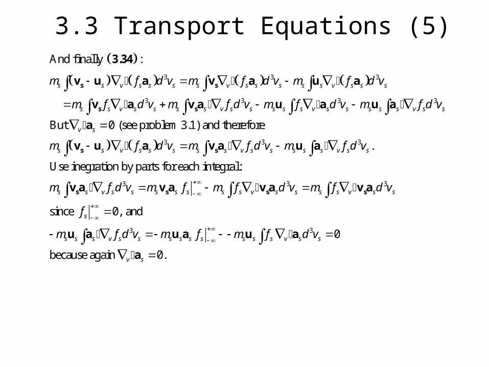
3.3 Transport Equations (5)

3 3 3

3 3 3 3

3

And finally :

But 0 (see problem 3.1) and therefore

s s v s s s s v s s s s s v s s s

s s v s s s s v s s s s s v s s s s s v s s

v s

s s v s s s

m f d v m f d v m f d v

m f d v m f d v m f d v m f d v

m f d v

s s

s s

s

3.34

v u a v a u a

v a v a u a u a

a

v u a

3 3

3 3 3

3

.

Use inegration by parts for each integral:

since 0, and

s s v s s s s s v s s

s s v s s s s s s s v s s s s v s s

s

s s s v s s s s s s s s s v

m f d v m f d v

m f d v m f m f d v m f d v

f

m f d v m f m f

s

s s s s

v a u a

v a v a v a v a

u a u a u

3 0

because again 0.

s s

v s

d v

a

a

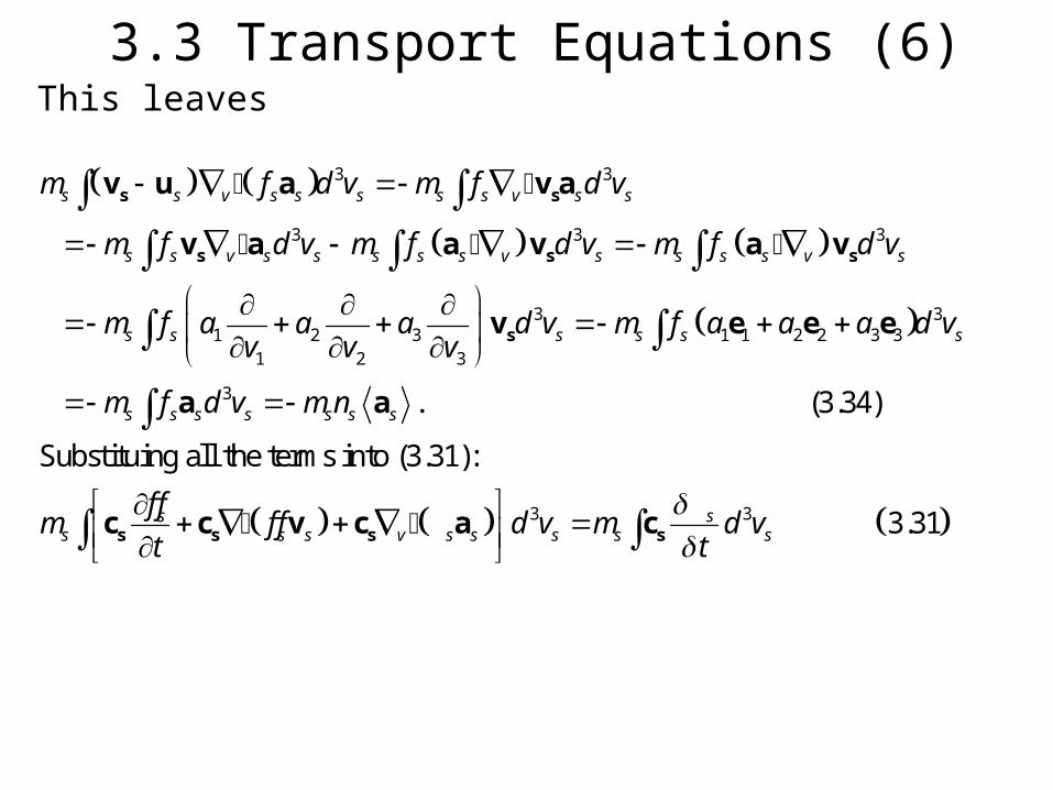
3.3 Transport Equations (6)This leaves

3 3

3 3 3

3 31 2 3 1 1 2 2 3 3

1 2 3

3 . (3.34)

Substituing all t

s s v s s s s s v s s

s s v s s s s s v s s s s v s

s s s s s s

s s s s s s s

m f d v m f d v

m f d v m f d v m f d v

m f a a a d v m f a a a d vv v v

m f d v m n

s s

s s s

s

v u a v a

v a a v a v

v e e e

a a

3 3

he terms into (3.31):

3.31s ss s s v s s s s s

f fm f f d v m d v

t t

s s s sc c v c a c

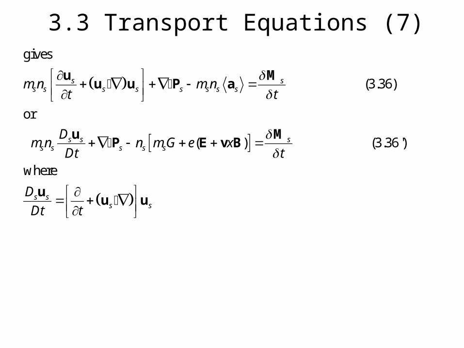
3.3 Transport Equations (7)

gives

(3.36)

or

( ) (3.36 ')

where

s ss s s s s s s s

s s ss s s s s

s ss s

m n m nt t

Dm n n m G e x

Dt t

D

Dt t

u Mu u P a

u MP E v B

uu u

Discussion of Transport Equations (8)

The momentum equation describes the evolution of the first-order velocity momentum us in terms of the second-order momentum Ps. Similarly the continuity equation describes the evolution of the density ns (zero-order momentum) using the first-order velocity momentum us, etc. This means, the transport equations are not a closed system.

To “close” the system we need an approximate distribution function fs(r,vs,t). We will use the local drifting Maxwellian.

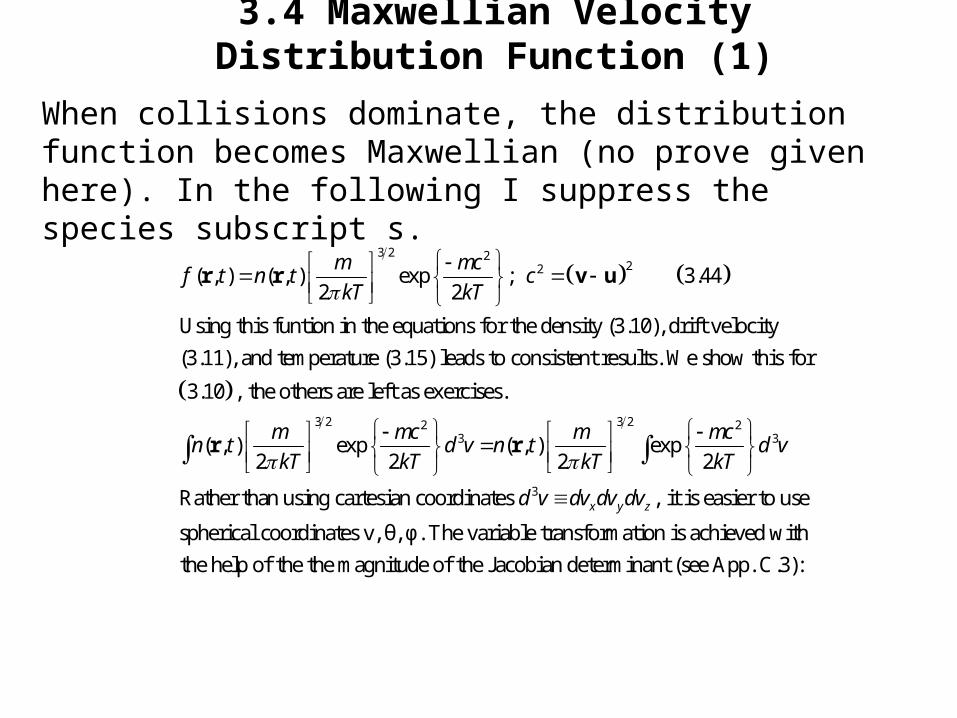
3.4 Maxwellian Velocity Distribution Function (1)

When collisions dominate, the distribution function becomes Maxwellian (no prove given here). In the following I suppress the species subscript s.

3 2 2

22( , ) ( , ) exp ; 3.442 2

Using this funtion in the equations for the density (3.10), drift velocity

(3.11), and temperature (3.15) leads to consistent results. We show this

m mcf t n t c

kT kT

r r v u

3 2 3 22 2

3 3

3

for

3.10 , the others are left as exercises.

( , ) exp ( , ) exp2 2 2 2

Rather than using cartesian coordinates , it is easier to use

sp

x y z

m mc m mcn t d v n t d v

kT kT kT kT

d v dv dv dv

r r

herical coordinates v, θ, φ. The variable transformation is achieved with

the help of the the magnitude of the Jacobian determinant (see App. C.3):

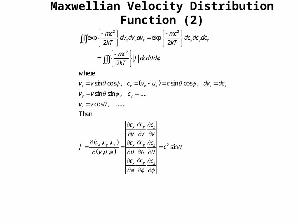
Maxwellian Velocity Distribution Function (2)

2 2

2

exp exp2 2

2

where

sin cos , sin cos ,

sin sin , ....

cos , .....

Then

( , , )

, ,

x y z x y z

x x x x x x

y y

z

yx z

x y z x

mc mcdv dv dv dc dc dc

kT kT

mcJ dcd d

kT

v v c v u c dv dc

v v c

v v

cc c

v v vc c c c

Jv

2 siny z

yx z

c cc

cc c

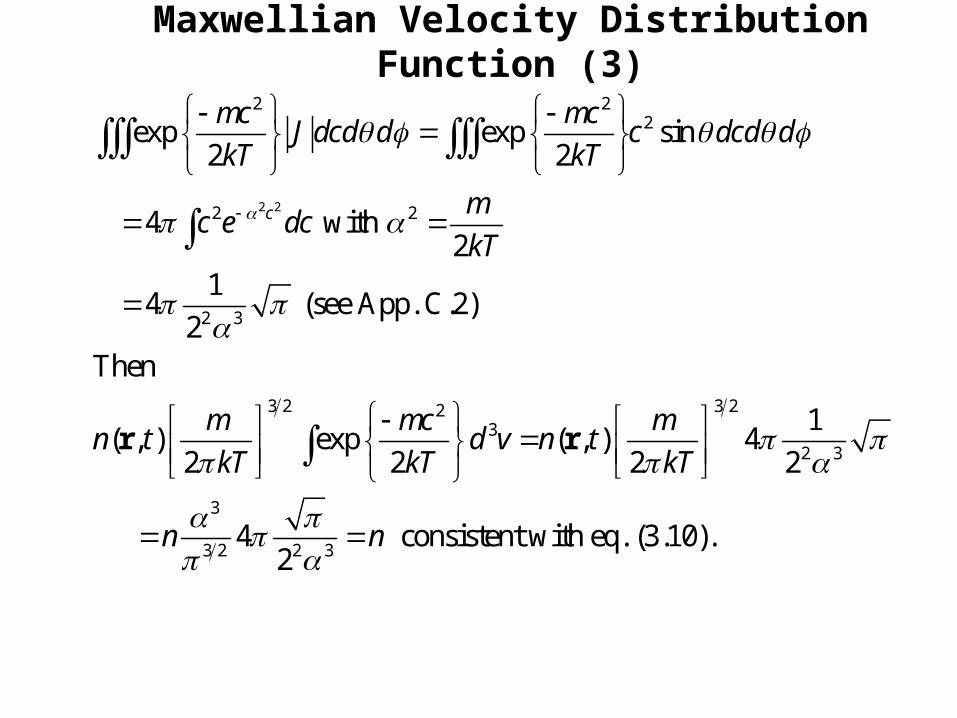
Maxwellian Velocity Distribution Function (3)

2 2

2 22

2 2

2 3

3 2 3 223

2 3

3

3 2 2 3

exp exp sin2 2

4 with 2

14 (see App. C.2)

2Then

1( , ) exp ( , ) 4

2 2 2 2

4 cons2

c

mc mcJ dcd d c dcd d

kT kT

mc e dc

kT

m mc mn t d v n t

kT kT kT

n n

r r

istent with eq. (3.10).

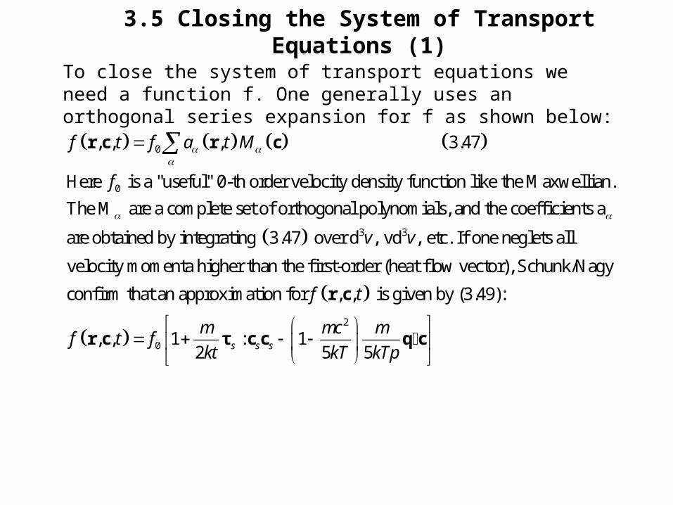
3.5 Closing the System of Transport Equations (1)

To close the system of transport equations we need a function f. One generally uses an orthogonal series expansion for f as shown below:

0

0

, , , 3.47

Here is a "useful" 0-th order velocity density function like the Maxwellian.

The M are a complete set of orthogonal polynomials, and the coefficients a

are obtained by integ

f t f a t M

f

r c r c

3 3

0

rating 3.47 over d , vd , etc. If one neglets all

velocity momenta higher than the first-order (heat flow vector), Schunk/Nagy

confirm that an approximation for , , is given by (3.49):

, , 1

v v

f t

f t f

r c

r c2

: 12 5 5s s s

m mc m

kt kT kTp

τ c c q c

3.5 Closing the System of Transport Equations (2)

1 1 1 2 1 3

11 12 13 1 1 1 2 1 3

21 22 23 2 1 2 2 2 3 2 1 2 3

31 32 33 3 1 3 2 3 3

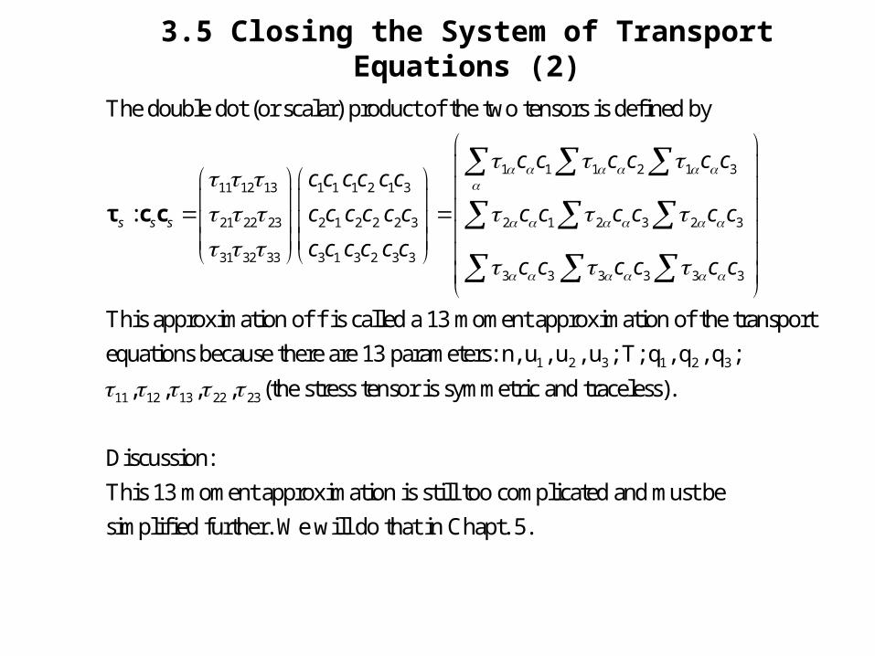
The double dot (or scalar) product of the two tensors is defined by

:s s s

c c c c c cc c c c c c

c c c c c c c c c c

c c c c c c

τ c c 2 3

3 3 3 3 3 3

1 2 3 1 2 3

1

This approximation of f is called a 13 moment approximation of the transport

equations because there are 13 parameters: n, u , u , u ; T; q , q , q ;

c c

c c c c c c

1 12 13 22 23, , , , (the stress tensor is symmetric and traceless).

Discussion:

This 13 moment approximation is still too complicated and must be

simplified further. We will do that in Chapt. 5.

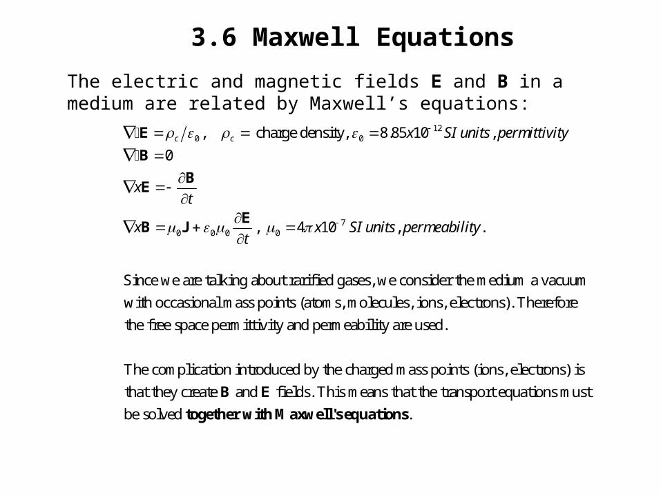
3.6 Maxwell Equations

The electric and magnetic fields E and B in a medium are related by Maxwell’s equations:

120 0

70 0 0 0

, charge density, 8.85 10 ,

0

, 4 10 , .

Since we are talking about rarified gases, we consider the medium a vacuum

w

c c x SI units permittivity

xt

x x SI units permeabilityt

E

B

BE

EB J

ith occasional mass points (atoms, molecules, ions, electrons). Therefore

the free space permittivity and permeability are used.

The complication introduced by the charged mass points (ions, electrons) is

that they create and fields. This means that the transport equations must

be solved .

B E

together with Maxwell's equations

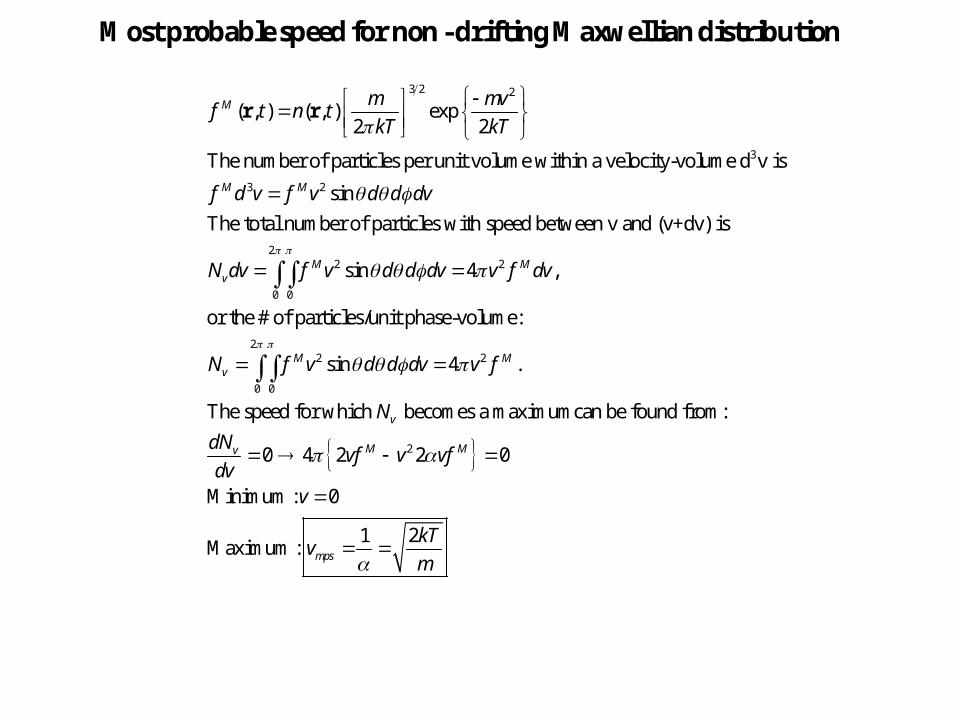
Most probable speed for non - drifting Maxwellian distribution

3 2 2

3

3 2

( , ) ( , ) exp2 2

The number of particles per unit volume within a velocity-volume d v is

sin

The total number of particles with speed between v and (v+dv) is

M

M M

m mvf t n t

kT kT

f d v f v d d dv

N

r r

22 2

0 0

22 2

0 0

2

sin 4 ,

or the # of particles/unit phase-volume:

sin 4 .

The speed for which becomes a maximumcan be found from:

0 4 2 2 0

Minimum : 0

M Mv

M Mv

v

M Mv

dv f v d d dv v f dv

N f v d d dv v f

N

dNvf v vf

dvv

1 2Maximum : mps

kTv

m