1

Lecture Notes PH 411/511 ECE 598 A. La Rosa

INTRODUCTION TO QUANTUM MECHANICS

PART- I The TRANSITION from CLASSICAL to QUANTUM PHYSICS ________________________________________________________________________

CHAPTER 3

The ORIGINS of QUANTUM PHYSICS

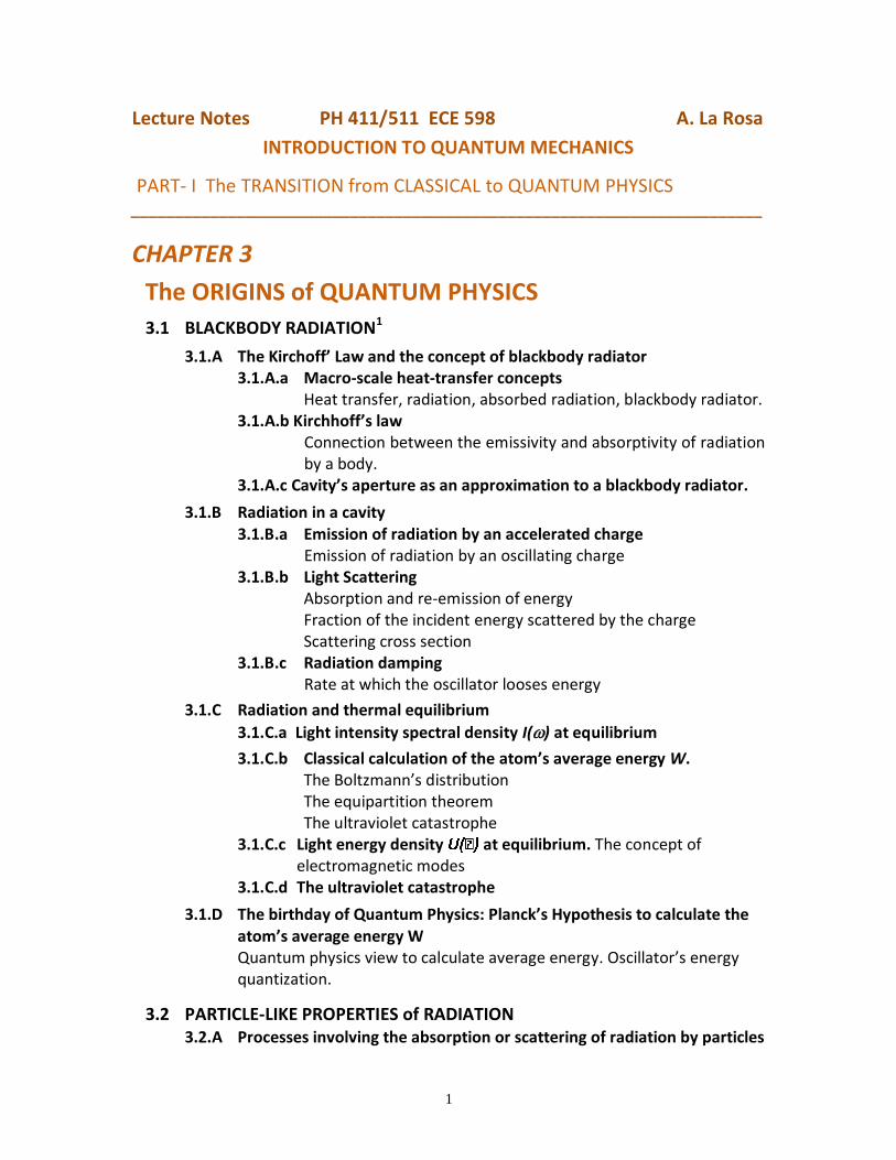
3.1 BLACKBODY RADIATION1

3.1.A The Kirchoff’ Law and the concept of blackbody radiator 3.1.A.a Macro-scale heat-transfer concepts

Heat transfer, radiation, absorbed radiation, blackbody radiator. 3.1.A.b Kirchhoff’s law

Connection between the emissivity and absorptivity of radiation by a body.

3.1.A.c Cavity’s aperture as an approximation to a blackbody radiator.

3.1.B Radiation in a cavity 3.1.B.a Emission of radiation by an accelerated charge

Emission of radiation by an oscillating charge 3.1.B.b Light Scattering

Absorption and re-emission of energy Fraction of the incident energy scattered by the charge Scattering cross section

3.1.B.c Radiation damping Rate at which the oscillator looses energy

3.1.C Radiation and thermal equilibrium

3.1.C.a Light intensity spectral density I() at equilibrium

3.1.C.b Classical calculation of the atom’s average energy W. The Boltzmann’s distribution The equipartition theorem The ultraviolet catastrophe

3.1.C.c Light energy density at equilibrium. The concept of electromagnetic modes

3.1.C.d The ultraviolet catastrophe

3.1.D The birthday of Quantum Physics: Planck’s Hypothesis to calculate the atom’s average energy W Quantum physics view to calculate average energy. Oscillator’s energy quantization.

3.2 PARTICLE-LIKE PROPERTIES of RADIATION 3.2.A Processes involving the absorption or scattering of radiation by particles

2

3.2.A.a Photoelectric effect. Einstein’s hypothesis of the quantized radiation energy

3.2.A.b Compton effect. Scattering of a complete quantum of radiation in definite direction.

3.2.A.c Pair production

3.2.B Processes where interacting charged particles produce radiation 3.2.B.a Brems-strahlung 3.2.B.b Pair annihilation

3.3 WAVE-LIKE PROPERTIES of PARTICLES 3.3.A The de Broglie Hypothesis

3.3.B Experimental confirmation of the de Broglie hypothesis. Electron

Diffraction

3.4 WAVE-PARTICLE DUALITY

References R. Eisberg and R. Resnick, “Quantum Physics,” 2nd Edition, Wiley, 1985.

Chapters 1 and 3 Richard Feynman, “The Feynman Lectures on Physics,”

Volume I, Chapter 32 and Chapter 41 (Section 41-2, 41-3)

3

CHAPTER 3

THE ORIGINS OF QUANTUM PHYSICS

By the end of the 19th century, classical physics appeared to be on solid foundations. The universe was conceive as containing matter consisting of

particles, obeying Newton’s law of motion; Einstein’s theory of special relativity generalized classical physics to include the region of high velocities.

and radiation (waves) obeying Maxwell’s equation of electromagnetism.

Some key experiments, however, could not be explained by classical physics, Blackbody Radiation

Photoelectric Effect Compton Effect

which forced the introduction of radical new concepts: Quantization of physical quantities

Particle properties of radiation Wave properties of particles

In the previous chapter we reviewed the strength of classical physics (electromagnetism and relativity.) In this chapter we aim to familiarize with the topics that forced a transition from classical to quantum concepts.

3.1 BLACKBODY RADIATION1

On December 14, 1900, at a meeting of the German Physical Society, Max Planck presented his paper “On the Theory of the Energy Distribution Law of the Normal Spectrum.” This date is considered to be the birthday of quantum physics. He broke ranks with the then quite accepted “law of equiparticion energy” that stated that the average energy of, for example, a harmonic oscillator was independent of its natural frequency. He instead postulated a frequency-dependent average energy and, very revolutionary, that the energy could have only discrete (quantized) values. Planck presented his paper while trying to explain the observed properties of thermal radiation. In this section we will review that development, as to gain some grasp of why the discreetness of a physical property lead to a radical different behavior of matter.

4

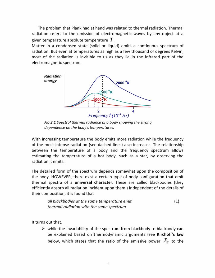
The problem that Plank had at hand was related to thermal radiation. Thermal radiation refers to the emission of electromagnetic waves by any object at a

given temperature absolute temperature .T Matter in a condensed state (solid or liquid) emits a continuous spectrum of radiation. But even at temperatures as high as a few thousand of degrees Kelvin, most of the radiation is invisible to us as they lie in the infrared part of the electromagnetic spectrum.

Radiation energy

Frequency f (1014

Hz) 4 2

1000 0K

1500 0K

2000 0K

Fig 3.1 Spectral thermal radiance of a body showing the strong dependence on the body’s temperatures.

With increasing temperature the body emits more radiation while the frequency of the most intense radiation (see dashed lines) also increases. The relationship between the temperature of a body and the frequency spectrum allows estimating the temperature of a hot body, such as a star, by observing the radiation it emits.

The detailed form of the spectrum depends somewhat upon the composition of the body. HOWEVER, there exist a certain type of body configuration that emit thermal spectra of a universal character. These are called blackbodies (they efficiently absorb all radiation incident upon them.) Independent of the details of their composition, it is found that

all blackbodies at the same temperature emit (1) thermal radiation with the same spectrum

It turns out that,

while the invariability of the spectrum from blackbody to blackbody can be explained based on thermodynamic arguments (see Kirchoff’s law

below, which states that the ratio of the emissive power eP to the

5

absorption coefficient a is the same for all bodies at the same temperature.)

the specific form of the spectrum (tending to zero at very low and very high frequencies) can not be explained in terms of classical physics arguments. (Planck was able to solve this problem on the basis of quantum arguments.)

Section 3.1 describes in more detail these two aspects.

3.1.A The Kirchoff’ Law and the Concept of Blackbody Radiator

3.1.A.a Macro-scale heat-transfer concepts

Heat transfer

While heat transfer Q by conduction and convection requires a

material medium, radiation does not.

Thermal Radiation

Refers to the emission of electromagnetic waves by any object at

a given temperature absolute temperature T .

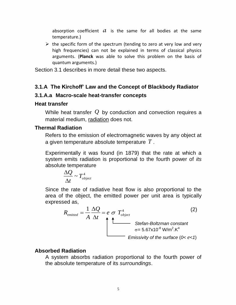
Experimentally it was found (in 1879) that the rate at which a system emits radiation is proportional to the fourth power of its absolute temperature

4~ objectT

t

Q

Since the rate of radiative heat flow is also proportional to the area of the object, the emitted power per unit area is typically expressed as,

41objectemitted Te

t

Q

AR

Emissivity of the surface (0< e<1)

Stefan-Boltzman constant

= 5.67x10-8 W/m2.K4

(2)

Absorbed Radiation A system absorbs radiation proportional to the fourth power of the absolute temperature of its surroundings.

6

4

gsurroundinabsorbed TaR

“a” indicates the relative ability of the

surface to absorb radiation (0< a<1)

(3)

For an object in equilibrium with its surrounding:

absorbedemitted RR , which implies ae (4)

That is,

Good radiators (e) are good absorbers (a) Heat flow via radiation from an object of area A to its surroundings

44

gssurroundinobject TTAet

Q

(5)

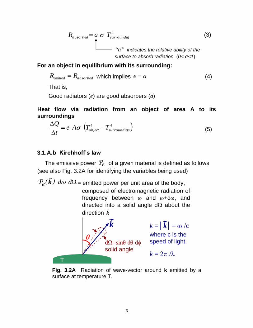
3.1.A.b Kirchhoff’s law

The emissive power eP of a given material is defined as follows

(see also Fig. 3.2A for identifying the variables being used)

dd)(Pe k

= emitted power per unit area of the body,

composed of electromagnetic radiation of

frequency between and +d, and

directed into a solid angle d about the

direction k

(6)

k

d=sin dd

solid angle

k =│k│= /c

where c is the speed of light.

k = /

T

Fig. 3.2A Radiation of wave-vector around k emitted by a surface at temperature T.

7

G. R. Kirchhoff proved in 1859 by using general thermodynamic arguments that, at any given electromagnetic wavelength,

the ratio of the emissive power eP to the absorption

coefficient a is the same for all bodies at the same temperature

etc321

aP

aP

aP eee

(6)

Blackbody Radiator

A perfect radiator would have an absorption (7) Coefficient a=1

Such a system is called a blackbody radiator

Note: The “blackbody” name of originates from the fact that “black looking” objects are in fact objects that do not reflect any of the incident light. “Black color” is in fact an absence of color. BUT in the context of the quantum physics that we are developing here, a blackbody radiator may not appear black at all. In fact, a blackbody emits very efficiently all colors.

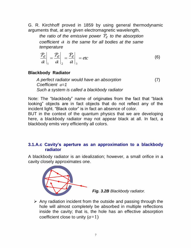
3.1.A.c Cavity’s aperture as an approximation to a blackbody radiator

A blackbody radiator is an idealization; however, a small orifice in a cavity closely approximates one.

Fig. 3.2B Blackbody radiator.

Any radiation incident from the outside and passing through the hole will almost completely be absorbed in multiple reflections inside the cavity; that is, the hole has an effective absorption

coefficient close to unity (a=1)

8

Since the cavity is in thermal equilibrium, the radiation getting inside through the small opening and that escaping from the small opening will be equal (e=1). We infer

that the spectral characteristics of the radiation emitted by the aperture should have then the characteristics of a blackbody radiator.

3.1.B Radiation in a cavity

Our next objective is to characterize the bath of electromagnetic radiation existent inside a blackbody radiator cavity. We would like to know,

How much light energy of angular frequency (across the electromagnetic spectrum) does exist inside the cavity at equilibrium conditions at a given temperature T?

(8)

Two approaches for answering this question, each arriving to the same general result, are worth mentioning:

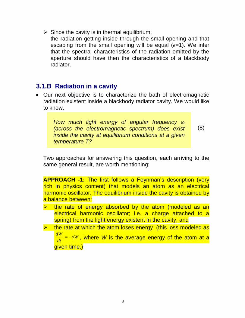
APPROACH -1: The first follows a Feynman‟s description (very rich in physics content) that models an atom as an electrical harmonic oscillator. The equilibrium inside the cavity is obtained by a balance between:

the rate of energy absorbed by the atom (modeled as an electrical harmonic oscillator; i.e. a charge attached to a spring) from the light energy existent in the cavity, and

the rate at which the atom loses energy (this loss modeled as

Wdt

dW , where W is the average energy of the atom at a

given time.)

9

Atom (modeled as an

harmonic oscillator)

Atom absorbs energy from the incident radiation

I()

Reflecting

walls

qe , me

ox : Amplitude of oscillation

Rate at which the atom (of average energy W) loses energy

Wdt

dW

Fig. 3.3 Atom (modeled as an electrical harmonic oscillator) in

equilibrium with a bath of electromagnetic radiation inside a box of perfectly reflecting walls. If it were not for the incident radiation, the atom‟s energy W would decay exponentially with time. A proper amount

of incident radiation I() allows W to remain constant. The objective in this section is to find out such proper amount of radiation; that is, so far

we do not know the I() that would permit equilibrium inside the box.

To calculate rate of energy absorbed by the atom from the incident radiation, we will appeal to the concept behind the process of scattering, in which the incident radiation drives the charge, and the latter re-emit it in all directions. This happens because

accelerated charges emit radiation. Calculating the power <P>

emitted by a charged particle emitted will allow, then, to calculate

the power absorbed by the atom from the incident radiation; they are the same.

That is, at equilibrium, <P> should be equal to W.

It is from the last equality that that an analytical expression will be

obtained for the required Light Intensity Spectral Density I() that must exist inside the cavity for an equilibrium situation to prevail.

APPROACH-2: The second approach is a bit more abstract; it

considers the energy-interchange equilibrium reached between the electromagnetic-modes inside the cavity and the cavity‟s walls.

10

It involves the counting of electromagnetic modes. An expression

for the Light Energy Density U() at equilibrium will be obtained.

The consistency of these two views will be verified through the

relationship I() = c U() where c is the speed of light.

It turns out that the procedure followed by these two approaches

(leading to an expression for I() and U() respectively) have survived the new wave of quantum concepts; that is, they are still considered valid. What has changed then?

What has changed dramatically, due to the advent of the quantum ideas, is the specific way to calculate the average-energy of an atom (in approach-1 method) or the average energy of an electromagnetic mode (approach-2 method.) A detailed description of these quantum modifications incurred in the

calculation of I() and U() constitutes the essence of Chapter 3.

In what follows, we will mainly concentrate on a detailed account of the approach-1 referred above. A description of the approach-2 is given in the appendix.

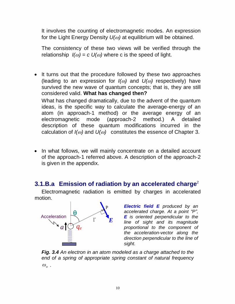
3.1.B.a Emission of radiation by an accelerated charge2

Electromagnetic radiation is emitted by charges in accelerated motion.

Electric field E produced by an accelerated charge. At a point “P”, E is oriented perpendicular to the line of sight and its magnitude proportional to the component of the acceleration-vector along the

direction perpendicular to the line of sight.

qe a E

r Acceleration

P

Fig. 3.4 An electron in an atom modeled as a charge attached to the end of a spring of appropriate spring constant of natural frequency

oω .

11

)/( 1

4

)sin(),(

2crta

rc

qtrE

o

e

Retardation time

(9) Electric field produced by an accelerated

charge qe

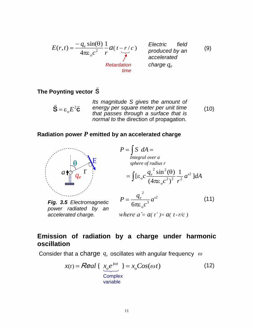
The Poynting vector S

Its magnitude S gives the amount of energy per square meter per unit time that passes through a surface that is normal to the direction of propagation.

cS

2Eo (10)

Radiation power P emitted by an accelerated charge

2

3

2

2

222

22

'6

]'1

)4(

)(sin[

ac

qP

dAarc

qc

dASP

o

e

o

eo

qe a

E r

Integral over a

sphere of radius r

where a’≡ a( t’ )= a( t - r/c )

(11) Fig. 3.5 Electromagnetic power radiated by an accelerated charge.

Emission of radiation by a charge under harmonic oscillation

Consider that a charge eq oscillates with angular frequency ω

)(} { )( tωCosxexalx o

tj

ot Re

Complex variable

(12)

12

Here, is not necessarily the natural frequency 0 ω of the oscillator

(see Fig 3.8). For example, the oscillator may be being driven by a external source of arbitrary frequency .

In what follows we will be evaluating time averages of physical

quantities (let‟s call it g ) over one period /2T of oscillation:

T

dttgT

g0

)(1

(13)

Notice, for example, that the time average of )( 2 tCos over one

period is ½.

We also will be using indistinctly )(ωtCos or . tωj

e For the latter it is

assume that we will take the real part after the calculations in order to obtain a proper (classical) physical interpretation.

From expression (11) we calculate an acceleration '2' tj

oexa

and 242

)(' 2/1 oxωa . Replacing these values in expression (11)

gives,

4

3

22

12

c

xq

o

oeP

Total average power emitted by a

charge eq undergoing harmonic

oscillations with amplitude ox ,

and angular frequency

(14)

3.1.B.b Light Scattering

Consider a plane wave (filling all the space) traveling in a specific

direction, let‟s say +X. Here we highlight only the temporal variation:

) (}

{ )( tCosEtωj

eERealt oo E (15)

time variation of the electric field of the incident radiation.

A traveling wave carries energy. A quantification of this travelling energy is expressed by the corresponding Poynting vector

cS

2Eo ; its average value, according to (12), is equal to,

2

2

1oocES (16)

13

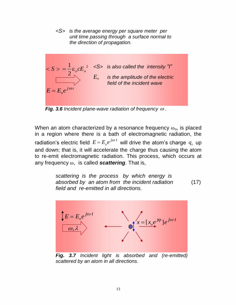
<S> is the average energy per square meter per unit time passing through a surface normal to the direction of propagation.

2

2

1oocES

t

o

jeEE

<S> is also called the intensity ”I”

Eo is the amplitude of the electric

field of the incident wave

Fig. 3.6 Incident plane-wave radiation of frequency .

When an atom characterized by a resonance frequency o, is placed in a region where there is a bath of electromagnetic radiation, the

radiation‟s electric field tj

eEE o

will drive the atom‟s charge eq up

and down; that is, it will accelerate the charge thus causing the atom to re-emit electromagnetic radiation. This process, which occurs at

any frequency , is called scattering. That is,

scattering is the process by which energy is absorbed by an atom from the incident radiation (17) field and re-emitted in all directions.

tjωeEE o

tjωeexx

jo ][

,

Fig. 3.7 Incident light is absorbed and (re-emitted) scattered by an atom in all directions.

14

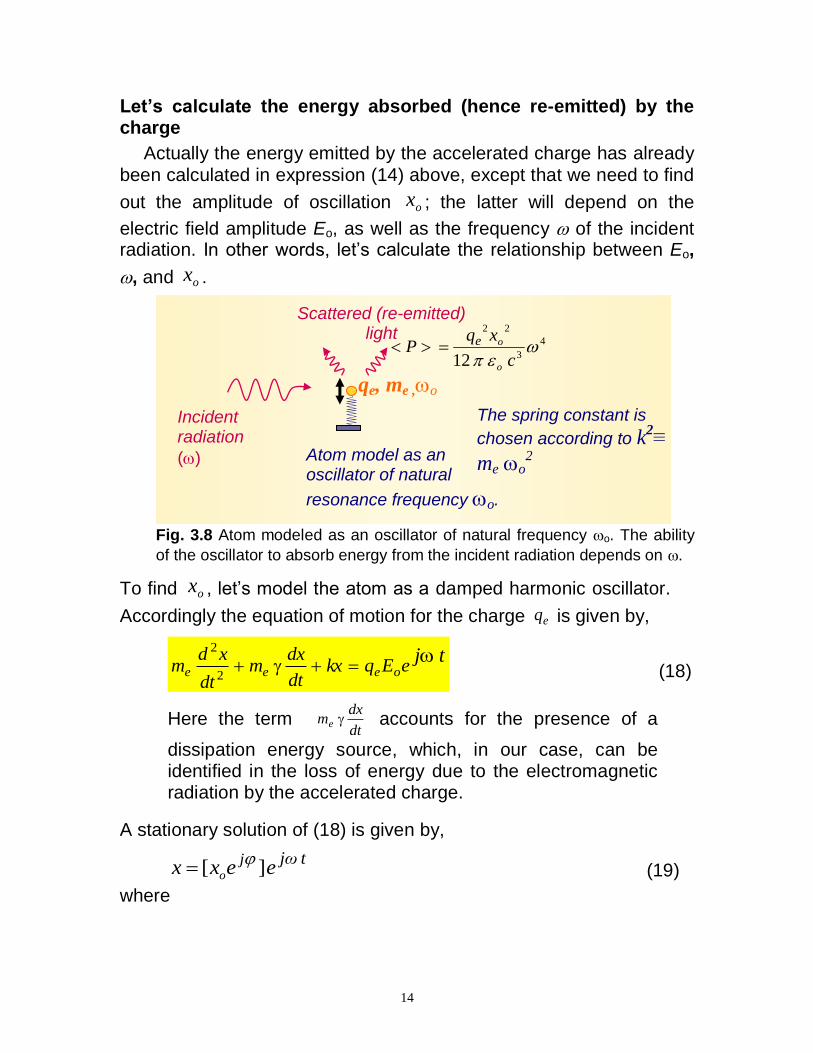
Let’s calculate the energy absorbed (hence re-emitted) by the charge

Actually the energy emitted by the accelerated charge has already

been calculated in expression (14) above, except that we need to find

out the amplitude of oscillation ox ; the latter will depend on the

electric field amplitude Eo, as well as the frequency of the incident radiation. In other words, let‟s calculate the relationship between Eo,

, and ox .

qe, me ,o

Scattered (re-emitted) light

Atom model as an oscillator of natural

resonance frequency o.

Incident radiation

()

The spring constant is

chosen according to k2≡

me o2

4

3

22

12

c

xqP

o

oe

Fig. 3.8 Atom modeled as an oscillator of natural frequency o. The ability

of the oscillator to absorb energy from the incident radiation depends on .

To find ox , let‟s model the atom as a damped harmonic oscillator.

Accordingly the equation of motion for the charge eq is given by,

tjeEqkx

dt

dxm

dt

xdm oeee

2

2

(18)

Here the term dt

dxme accounts for the presence of a

dissipation energy source, which, in our case, can be identified in the loss of energy due to the electromagnetic radiation by the accelerated charge.

A stationary solution of (18) is given by,

tjωeexx

jo ][

(19)

where

15

2/1

22222 )(

)/()(

o

oeeoo

Emqωxx

(20) Amplitude of oscillation as a function of frequency

and

tan

22

1

o

(20)‟

Expression (20) indicates that the amplitude of oscillation xo (and

hence the acceleration) of the charge depends on the incident

radiation‟s frequency .

Let‟s proceed now to calculate the total power radiate by the accelerated charge under the influence of an electric filed of

amplitude E0 and frequency . Replacing the value of xo given in (20)

for xo into the expression for the radiation power 4

3

22

12

c

xqP

o

oe

given in (14), one obtains, )()(

)/(

12 2222

224

3

2

ωωω

Emqω

c

qP

o

oee

o

e

.

Rearranging terms,

)()( 43

8

2

12222

42

2

22

)(

oeo

eoo

cm

qcEP (21)

Expression (21) gives the total average energy emitted by the charge qe when subjected to a harmonic electric field (given in expression

(15) )of amplitude E0 and frequency .

Notice the expression 2

2

1oocE (incident energy per unit area per

second, i.e. the incident intensity Io) has been factored out in expression (21). This is convenient, for it allows to interpret (21) the following way: Out of the incident intensity Io present in the cavity, a

„fraction‟ of it equal to ) ()( 2222

42

2

2

)(43

8

oeo

e

cm

q is present in the

form of scattered power. We say „fraction‟ because the units of that

16

last expression is area (not a simple fraction number). Hence, it is better to interpret (21) in terms of “scattering cross section).

The concept of scattering cross section

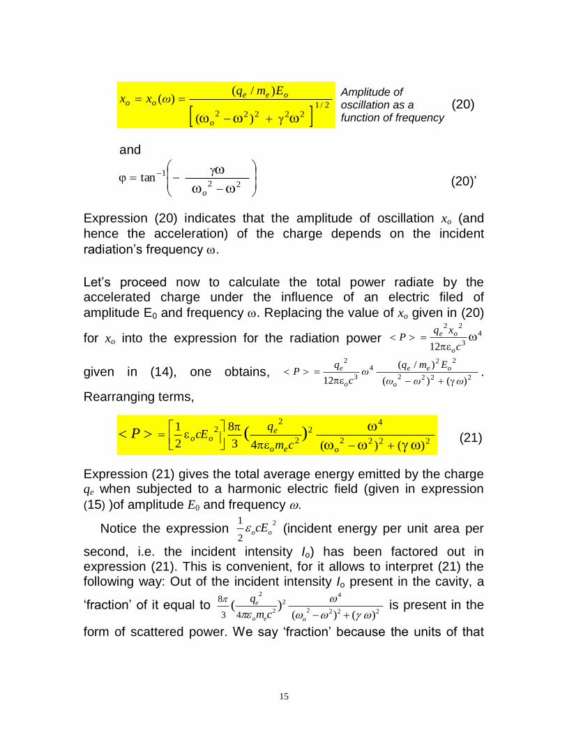
If we considered a hypothetical cross section of area intersecting the incident radiation, the amount of energy per second hitting that area would be

IcEP oo ]2

1[

2

(22)

2

2

1oocES

cross section

of area

<S> is called the

light intensity I Fig. 3.9 Pictorial representation of scattering cross section.

One can use the analogy of an affective area being intercepted by the incident radiation to define how effectively the radiation is absorbed and scattered (i. e. re-emitted) by an atom. In effect, comparing expressions (21) and (22), the total power scattered by an atom is numerically equal to the energy per second incident on a “surface” of

cross-section area scattering ,

scatteringooscattering cEP ]2

1[

2 (23)

where

2222

42

2

2

)()()

4(

3

8

oeo

escattering

cm

q (24)

scattering has units of area.

17

scattering

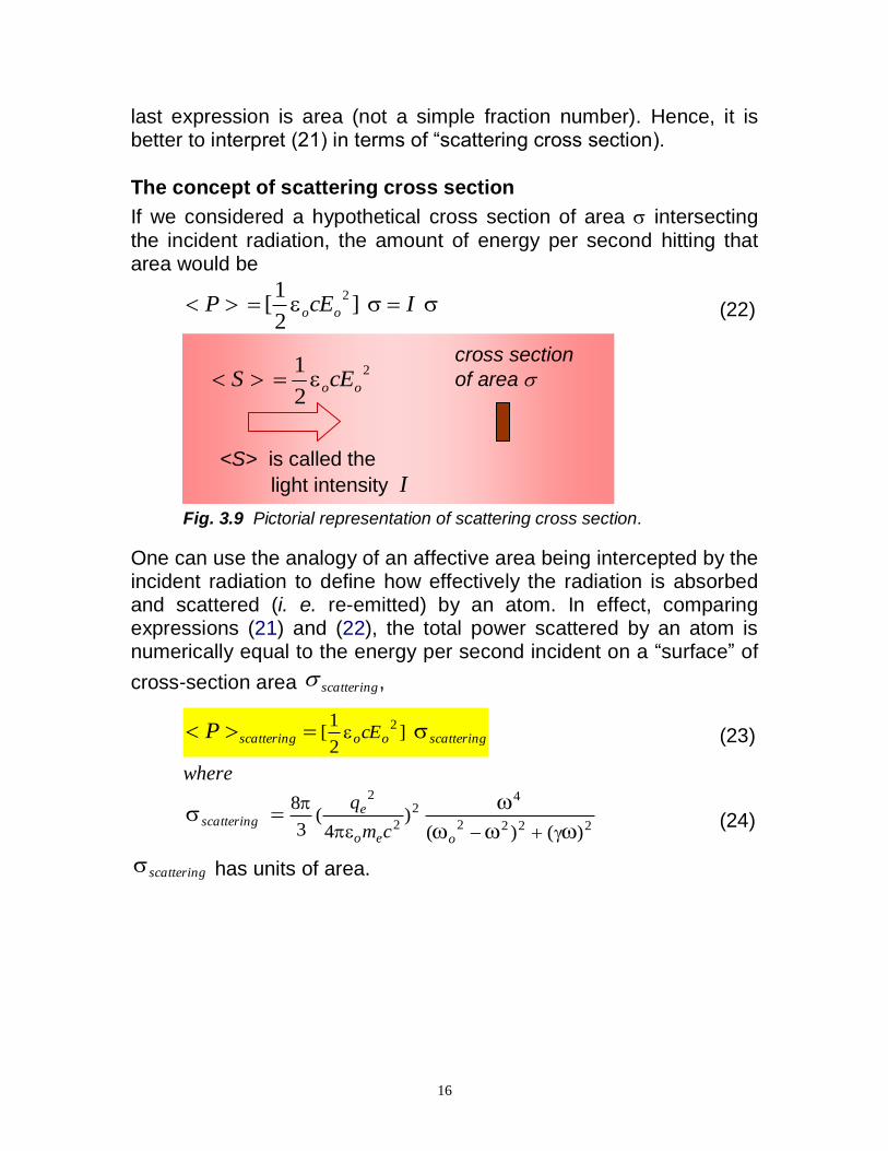
Fig.3.10 Sketch of the atom’s scattering cross section.

Put it differently, if we have a collimated beam travelling across the space in the, let‟s say, x-direction, the sideway regions will be dark. One way to illuminate the sideways is to intercept the beam with an atom, which will scatter the light. But out of Io the amount of power

that will be scattered is Io , no more, no less. That is s is an indicator of the ability of the atom to absorb (and hence scatter) the light. We cannot ask, we cannot expect, the atom to scatter more

than Io (where is given by expression (24)).

Certainly, every photon absorbed by the atom will be scattered out.

But what expression (24) is suggesting is that photons of frequency

quite different than o will have little chance to be absorbed (and re-

emitted.) The closer is to o, the higher the chances to be absorbed (and subsequently be re-emitted.)

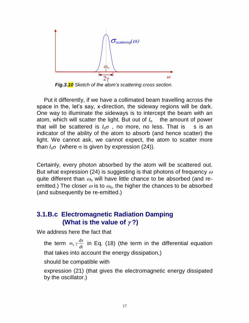
3.1.B.c Electromagnetic Radiation Damping

(What is the value of ?)

We address here the fact that

the term dt

dxme in Eq. (18) (the term in the differential equation

that takes into account the energy dissipation,)

should be compatible with

expression (21) (that gives the electromagnetic energy dissipated by the oscillator.)

18

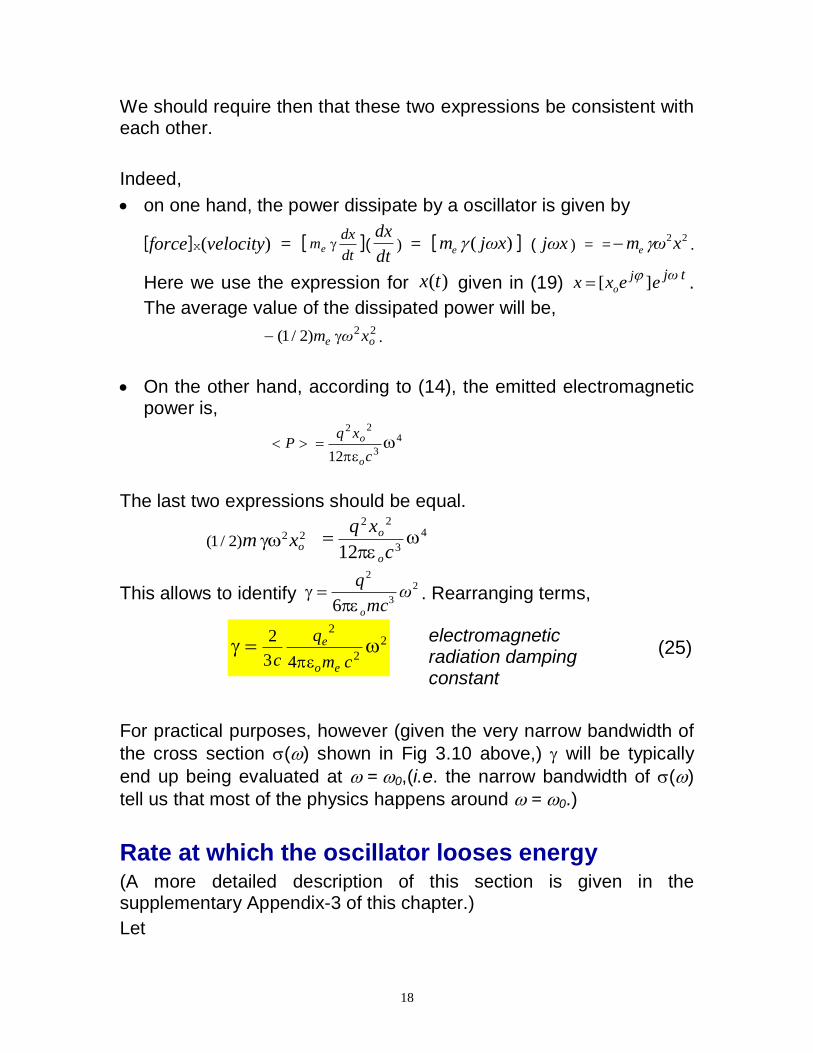
We should require then that these two expressions be consistent with each other.

Indeed,

on one hand, the power dissipate by a oscillator is given by

[force]x(velocity) = [dt

dxme ](

dt

dx) = [ )( xjωme ] ( xjω ) = =

22 xωme .

Here we use the expression for )(tx given in (19) tjω

eexxj

o ][

.

The average value of the dissipated power will be,

22 )2/1( oe xωm .

On the other hand, according to (14), the emitted electromagnetic power is,

4

3

22

12

c

xqP

o

o

The last two expressions should be equal.

22 )2/1( oxm

4

3

22

12

c

xq

o

o

This allows to identify 2

3

2

6ω

mc

q

o . Rearranging terms,

2

2

2

43

2

cm

q

ceo

e

electromagnetic radiation damping constant

(25)

For practical purposes, however (given the very narrow bandwidth of

the cross section () shown in Fig 3.10 above,) will be typically

end up being evaluated at =0,(i.e. the narrow bandwidth of ()

tell us that most of the physics happens around =0.)

Rate at which the oscillator looses energy (A more detailed description of this section is given in the supplementary Appendix-3 of this chapter.)

Let

19

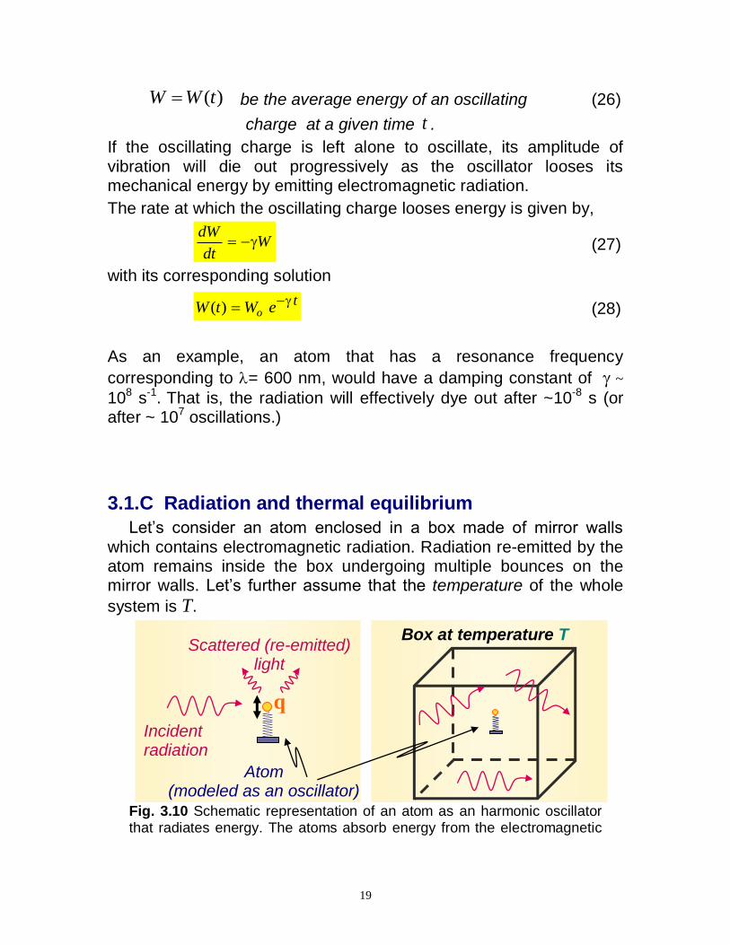
)(tWW be the average energy of an oscillating (26)

charge at a given time t .

If the oscillating charge is left alone to oscillate, its amplitude of vibration will die out progressively as the oscillator looses its mechanical energy by emitting electromagnetic radiation.

The rate at which the oscillating charge looses energy is given by,

Wdt

dW (27)

with its corresponding solution

teWtW o

)(

(28)

As an example, an atom that has a resonance frequency

corresponding to = 600 nm, would have a damping constant of ~

108 s-1. That is, the radiation will effectively dye out after ~10-8 s (or after ~ 107 oscillations.)

3.1.C Radiation and thermal equilibrium

Let‟s consider an atom enclosed in a box made of mirror walls which contains electromagnetic radiation. Radiation re-emitted by the atom remains inside the box undergoing multiple bounces on the mirror walls. Let‟s further assume that the temperature of the whole

system is T.

q

Scattered (re-emitted) light

Box at temperature T

Atom (modeled as an oscillator)

Incident radiation

Fig. 3.10 Schematic representation of an atom as an harmonic oscillator that radiates energy. The atoms absorb energy from the electromagnetic

20

radiation existent inside the box (the latter assumed to be made of perfectly reflecting walls.)

How to make the temperature T intervene in an expression like (14)

that gives the power scattered by an atom in the form

scatteringP 4

3

22

12

c

xq

o

oe

?

It is plausible to assume that the equilibrium temperature should correspond to proper value of the amplitude of the electric field,

oE , since the higher the value of oE , the higher the charge‟s

amplitude of vibration xo, the greater temperature to be associated

with the atom (i.e. the amplitude of the oscillator should increase with temperature.) If our assumption were correct, how to find then the proper value

of oE corresponding to a given temperature T?

Aiming to find a proper answer let‟s outline some considerations:

- If an atomic oscillator had no charge, it would oscillate forever. It would have an average energy W compatible with the temperature

in the box; that is )( TWW . In other words, it would oscillate

forever with an amplitude settled by the temperature T in the box.

½ k xo2 = ½ kT or ½ mo

2xo

2 = ½ kT.

- But our atomic oscillator is charged. If it were left alone, its amplitude of vibration xo would die out progressively, as the

oscillator looses its energy by emitting electromagnetic radiation.

- If our atomic charged oscillator were in physical contact with other atoms, energy in the proper amount will be supplied by their mutual collisions as to keep the same temperature among themselves. Here, however, we will consider that the energy is supplied via electromagnetic interaction: the atom draws energy from the radiation existent in the cavity to compensate the energy being lost by radiation (accelerated charged particles emit radiation.) When this compensation of energy matches, then we are at an

equilibrium situation, which inherently should occur at a given temperature (the latter settling the charge‟s amplitude of oscillation

21

at a corresponding value.) We will retake the subject of temperature dependence of x0 in Section 3.1.c.b below.

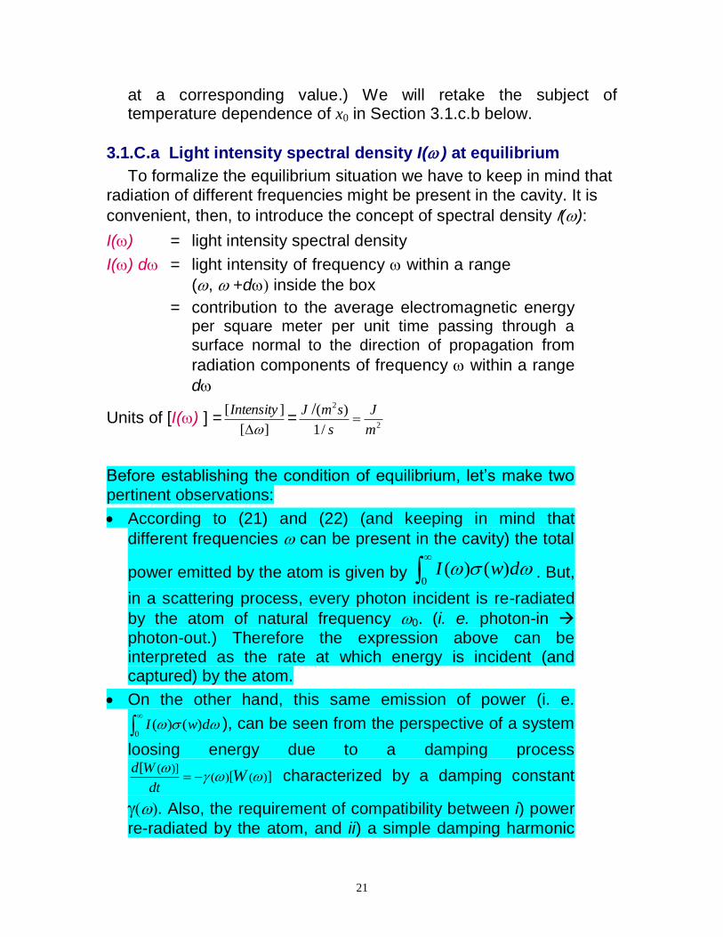
3.1.C.a Light intensity spectral density I() at equilibrium

To formalize the equilibrium situation we have to keep in mind that radiation of different frequencies might be present in the cavity. It is

convenient, then, to introduce the concept of spectral density I():

I() = light intensity spectral density

I() d = light intensity of frequency within a range

(, +d inside the box

= contribution to the average electromagnetic energy per square meter per unit time passing through a

surface normal to the direction of propagation from

radiation components of frequency within a range

d

Units of [I() ] =][

][

Intensity=

2

2

/1

)(/

m

J

s

smJ

Before establishing the condition of equilibrium, let‟s make two pertinent observations:

According to (21) and (22) (and keeping in mind that

different frequencies can be present in the cavity) the total

power emitted by the atom is given by

0)()( dwI . But,

in a scattering process, every photon incident is re-radiated

by the atom of natural frequency 0. (i. e. photon-in photon-out.) Therefore the expression above can be interpreted as the rate at which energy is incident (and captured) by the atom.

On the other hand, this same emission of power (i. e.

0)()( dwI ), can be seen from the perspective of a system

loosing energy due to a damping process

][[

)()()](

Wdt

Wd characterized by a damping constant

. Also, the requirement of compatibility between i) power

re-radiated by the atom, and ii) a simple damping harmonic

22

oscillator model tjeEqkx

dt

dxm

dt

xdm oeee

2

2

, lead to

expression (25) 2

2

2

43

2

cm

q

c eo

e)( . But since all the

dynamics occurs at , that is W()~0 for ≠ , we can

use WW

odt

d)( , with the interpretation that W is the total

energy of the atom.

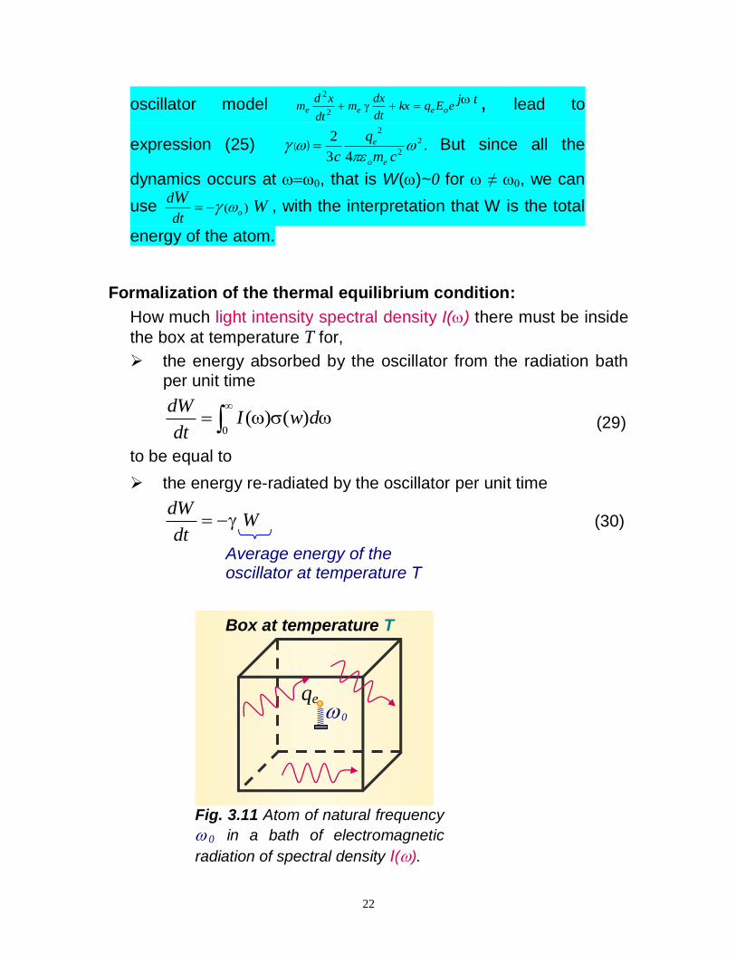
Formalization of the thermal equilibrium condition:

How much light intensity spectral density I() there must be inside

the box at temperature T for,

the energy absorbed by the oscillator from the radiation bath per unit time

0

)()( dwIdt

dW (29)

to be equal to

the energy re-radiated by the oscillator per unit time

Wdt

dW

Average energy of the oscillator at temperature T

(30)

Box at temperature T

0 qe

Fig. 3.11 Atom of natural frequency

0 in a bath of electromagnetic

radiation of spectral density I().

23

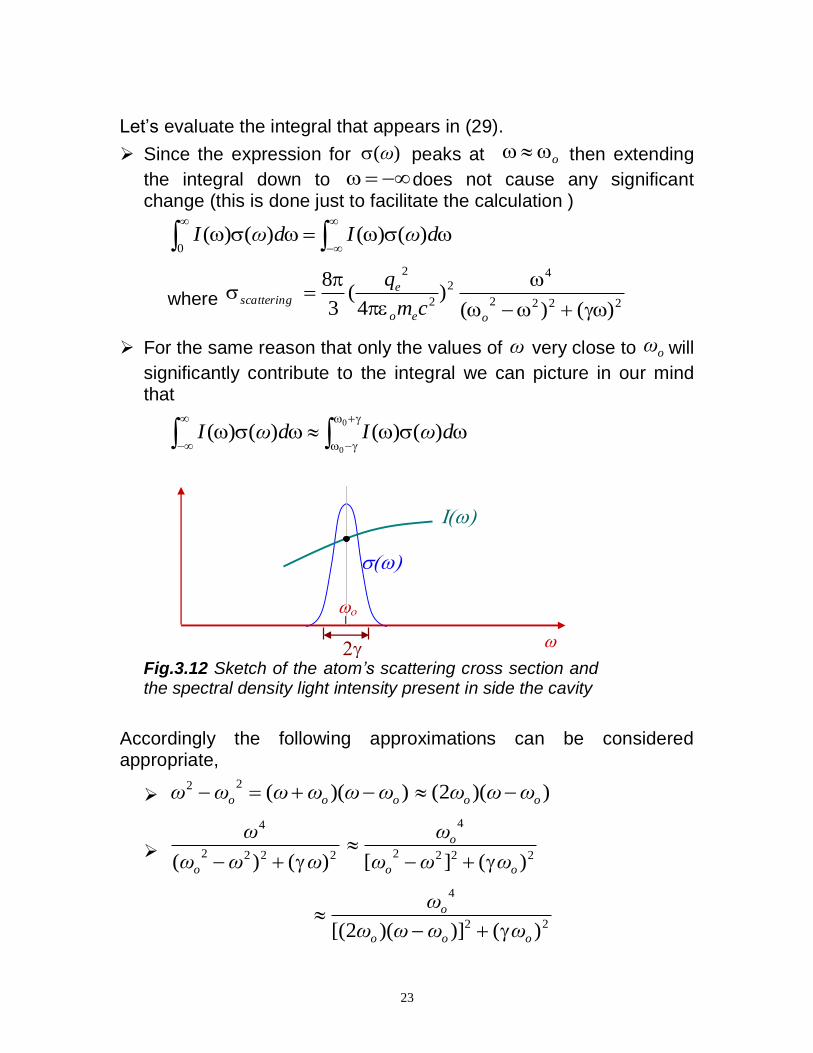
Let‟s evaluate the integral that appears in (29).

Since the expression for )(ω peaks at o then extending

the integral down to does not cause any significant change (this is done just to facilitate the calculation )

dωIdωI )()()()(0

where 2222

42

2

2

)()()

4(

3

8

oeo

escattering

cm

q

For the same reason that only the values of ω very close to oω will

significantly contribute to the integral we can picture in our mind that

0

0

)()()()( dωIdωI

A(k)

Fig.3.12 Sketch of the atom’s scattering cross section and the spectral density light intensity present in side the cavity

Accordingly the following approximations can be considered appropriate,

22

oωω ))(( oo ωωωω ))(2( oo ωωω

2222

4

)()( ωωω

ω

o 2222

4

)(][ oo

o

ωωω

ω

22

4

)()])(2[( ooo

o

ωωωω

ω

24

22

2

)(4

o

o

ωω

ω

)()( oII

All these approximations lead to

dωIdωI )()()()(0

d

cm

qI

oeo

e

2222

42

2

2

)()()

4(

3

8)(

d

ωω

ω

cm

qI

o

o

eo

e

22

2

2

2

2

)(4)

4(

3

8)(

d

ωωω

cm

qωI

o

o

eo

e

o

22

22

2

2

)2/()(

1)

4(

3

2)(

(using a

x

aax

dxarctan

1

22

)

)( )2

(2

2/

1)

4(

3

2)(

22

2

2

o

eo

e

o ωcm

qωI

2)

4(

3

2)(

22

2

2

o

eo

e

o ωcm

qωI

22

2

22

0)(

43

2)()()( o

eo

eo ω

cm

qωIdωI

(31)

At equilibrium we should have,

0

)()( dwIdt

dW = W

dt

dW , which

leads to

Wωcm

qωI o

eo

e

o

22

2

22

)(43

2)(

W

ωq

cmωI

oe

eoo 2

22

2

2

2)(

4

2

3)(

25

Using expression (25) for the value of 2

2

2

43

2ω

cm

q

co

evaluated

at 0ωω one obtains,

Wωcm

q

cq

cmωI o

oe

eoo

22

2

22

2

2

2)

43

2(

4

2

3)(

)(

, or

Wω

cωI oo

22

2)

3

2(

2

3)(

,

Wωc

ωI oo 3

1)(

2

22 (32)

Average energy of the oscillator

I() is the light spectral density at =.

Here is the natural frequency of the oscillator we were focusing in. Had we used an oscillator of a different natural frequency, let‟s say

‟, we would have obtained a similar expression (32) but with ‟

instead of . Hence, in general,

Average energy of the oscillator at temperature T

Wωc

ωI 3

1)( 2

22 (32)‟

Required light intensity spectral density I()

inside the box at temperature T in order to

maintain equilibrium.

Notice

Units of [I() d] = ][Intensity =sm

J2

Units of [I() ] =][

][

Intensity=

2

2

/1

)(/

m

J

s

smJ

It is worth to highlight that,

26

Expression (32)‟ has remained undisputed. That is, it is still considered correct even when the new quantum mechanics concepts are introduced.

It is in the calculation of the average energy W where the classical

and quantum approaches fundamentally diverge.

3.1.C.b Classical calculation of the atom’s average energy W.

In classical statistical mechanics there exists a very general result so called “equipartition theorem,” which states that the mean value of a quadratic term in the energy is equal to ½ kBT. Here kB is the Boltzmann‟s constant and T is the absolute temperature.

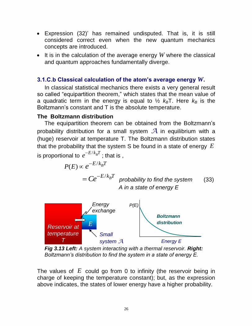
The Boltzmann distribution The equipartition theorem can be obtained from the Boltzmann‟s

probability distribution for a small system A in equilibrium with a

(huge) reservoir at temperature T. The Boltzmann distribution states

that the probability that the system S be found in a state of energy E

is proportional to TkE

Be/

; that is ,

TkE BeEP/

)(

TkE BCe

/ probability to find the system (33)

A in a state of energy E

E Reservoir at temperature

T

Energy exchange

Energy E

P(E)

Boltzmann

distribution

Small

system A Fig 3.13 Left: A system interacting with a thermal reservoir. Right: Boltzmann’s distribution to find the system in a state of energy E.

The values of E could go from 0 to infinity (the reservoir being in charge of keeping the temperature constant); but, as the expression above indicates, the states of lower energy have a higher probability.

27

Since for a given energy there may be several states characterized by the same energy, it is usual to define,

dEEg )( number of states with energy (34)

E , within an interval dE , thus giving

dEEgCTkE Be )(

/ probability to find the system A

in a state of energy between E

and E+ dE,

which suggests to rather identify a probability-density )(EP defined as follows

dEEgCdEETkE Be )()(

/P the probability to find the (35)

system in a state of energy between E and

E+ dE,

with C being a constant to be determined.

Since the probabilities added over all the possible states should be

equal to 1, we must require, 1')'(0

/'

dEEgC

TkE Be , which gives,

1C =

0

/' TkE Be ')'( dEEg (36)

A self consistent expression for )(EP is therefore given by,

0'

)()(

)'(/'

/

dEEgTkE

TkE

B

B

e

e dEEgdEEP

(37)

(Notice in the denominator we are using a „dummy‟ variable 'E .)

From expression (37) we can formally calculate the average energy of the system,

0

0

')'(

)(

/'

/

dEEg

dEEgEE

TkE

TkE

B

B

e

e

(38)

The Equipartition Theorem

28

It turns out, very often the energy of the system may contain a quadratic term. Consider for example

... 2

1

2

2

2

kxm

pE x

,

and we would like to calculate, for example, the average value of the

kinetic energy term m

px

2

2

alone. As we know, being the system in

contact with a heat reservoir, the value of m

px

2

2

is sometimes high,

sometimes it is low because it gains or looses energy from the heat reservoir; we would like to know what would be its average value

m

px

2

2

.

0

2

0

2

2

2

/

/

2

2

2

2x

Bm

x

x

Bm

xx

x

dp

dpm

p

m

p

Tk

Tk

p

p

e

e

(39)

Let‟s call

TkB

1 (40)

In terms of expression (39) becomes,

0

2

0

2

0

2

0

2

2

2

2

2

2

2

2

2

xm

x

xm

x

xm

x

xm

xx

x

dp

dpβ

dp

dpm

p

m

p

p

p

p

p

β

β

β

β

e

e

e

e

0

2

0

2

2

2

xm

x

xm

x

dp

dpβ

p

p

β

β

e

e

0

2

22

ln2

xm

xx dp

βm

pp

βe (41)

Defining the variable xpm

βu

2 ,

29

00

222

21

ln 2

ln2

dumβ

dum

βm

p uu eex

0

22

2ln1

ln2

dumβm

p uex

Term independent of

2

1ln

2

1

2

2

βm

px

Tkm

pB

x

2

1

2

2

(42)

Had we chosen any other quadratic term of the energy we would have obtained the same result. This is the equipartition theorem. It states that the mean value of each independent quadratic term in the

energy is equal to TkB2

1.

The ultraviolet catastrophe

Using this result (42) in expression (32) WI oo ωc

ω 3

1)(

2

22 , the

different degrees of freedom (let‟s assume there are f different

quadratic terms in the expression for the total energy) involved in the

calculation of W would lead to a finite number f of TkB2

1. Thus,

Tkfωc

ω BooI2

1

3

1)(

2

22 . Since the value of oω is accidental (we

would obtain a similar expression if we were to choose an atom of different resonance frequency), we have the following result,

6

)( 2

22ω

c

Tkfω BI

classical prediction (43)

30

I()

Frequency

Classical prediction Experimental

results

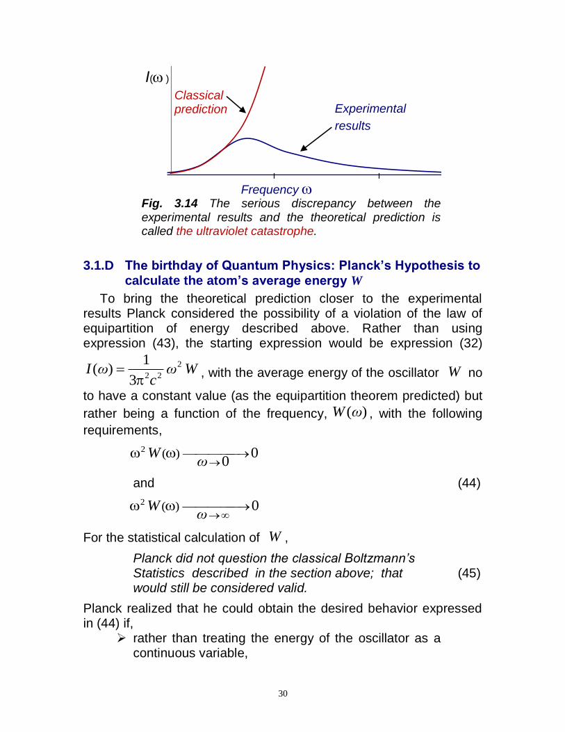
Fig. 3.14 The serious discrepancy between the experimental results and the theoretical prediction is called the ultraviolet catastrophe.

3.1.D The birthday of Quantum Physics: Planck’s Hypothesis to calculate the atom’s average energy W

To bring the theoretical prediction closer to the experimental results Planck considered the possibility of a violation of the law of equipartition of energy described above. Rather than using expression (43), the starting expression would be expression (32)

Wωc

ωI 3

1)( 2

22 , with the average energy of the oscillator W no

to have a constant value (as the equipartition theorem predicted) but

rather being a function of the frequency, )( ωW , with the following

requirements,

00

)( 2

ω

W

and (44)

0

)( 2

ω

W

For the statistical calculation of W ,

Planck did not question the classical Boltzmann’s Statistics described in the section above; that (45) would still be considered valid.

Planck realized that he could obtain the desired behavior expressed in (44) if,

rather than treating the energy of the oscillator as a continuous variable,

31

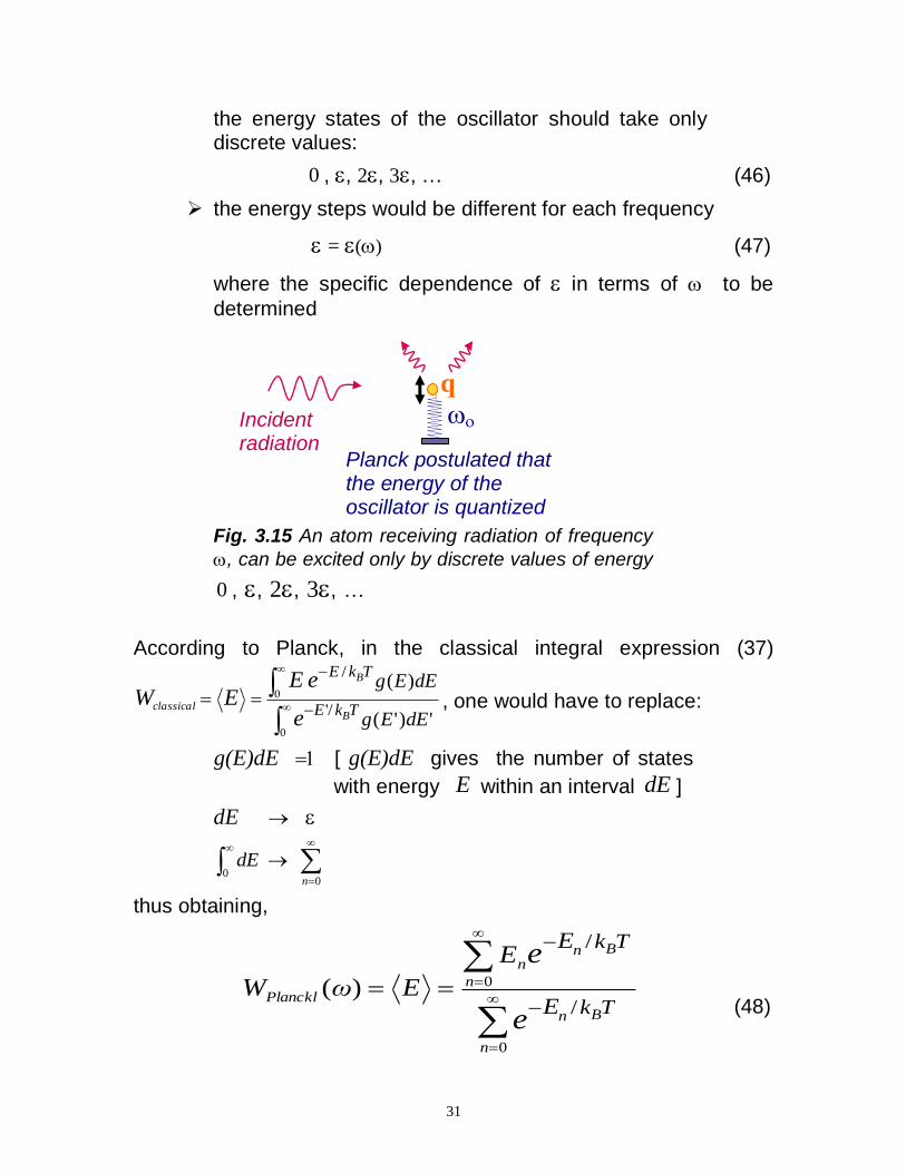
the energy states of the oscillator should take only discrete values:

0 , , 2, 3, … (46)

the energy steps would be different for each frequency

= () (47)

where the specific dependence of in terms of to be

determined

q

Incident radiation

Planck postulated that the energy of the oscillator is quantized

Fig. 3.15 An atom receiving radiation of frequency

, can be excited only by discrete values of energy

0 , , 2, 3, …

According to Planck, in the classical integral expression (37)

0

0

')'(

)(

/'

/

dEEg

dEEg

TkE

TkE

B

B

classical

e

eEEW , one would have to replace:

g(E)dE [ g(E)dE gives the number of states

with energy E within an interval dE ]

dE

0

0

n

dE

thus obtaining,

0

0

/

/

)(

n

Bn

Bn

n

n

PlancklTk

Tk

E

E

e

eE

EωW (48)

32

where nE = n() ; n= 1 2, 3, …

A graphic illustration can help understand why this hypothesis could indeed work:

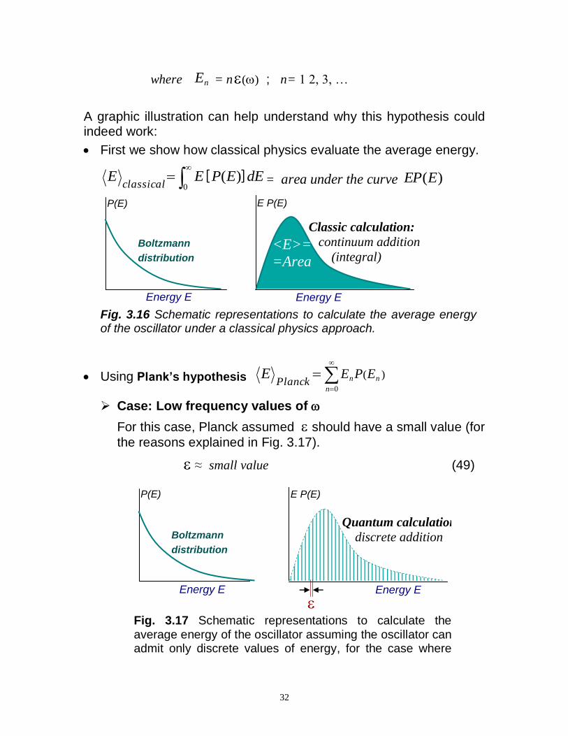
First we show how classical physics evaluate the average energy.

0

)( dEEPEEclassical

][ = area under the curve )(EEP

Energy E

P(E)

Boltzmann

distribution

Energy E

E P(E)

<E>=

=Area

Classic calculation:

continuum addition

(integral)

Fig. 3.16 Schematic representations to calculate the average energy of the oscillator under a classical physics approach.

Using Plank’s hypothesis Planck

E )(

0

n

n

n EPE

Case: Low frequency values of

For this case, Planck assumed should have a small value (for

the reasons explained in Fig. 3.17).

≈ small value (49)

Energy E

P(E)

Boltzmann

distribution

Energy E

E P(E)

<E>=

=Area

~kB T

Quantum calculation:

discrete addition

Fig. 3.17 Schematic representations to calculate the average energy of the oscillator assuming the oscillator can admit only discrete values of energy, for the case where

33

the separation between contiguous energy levels being of relatively low value.

Indeed, comparing Fig. 3.16 and Fig 3.17 one notices that if

is small then the value of )(

0

n

n

n EPE

will be very close to the

classical value.

It is indeed desirable that Planck‟s results agree with the classic results at low frequencies, since the classical predictions and the experimental results agree well at low frequencies (see Fig. 3.14 above.)

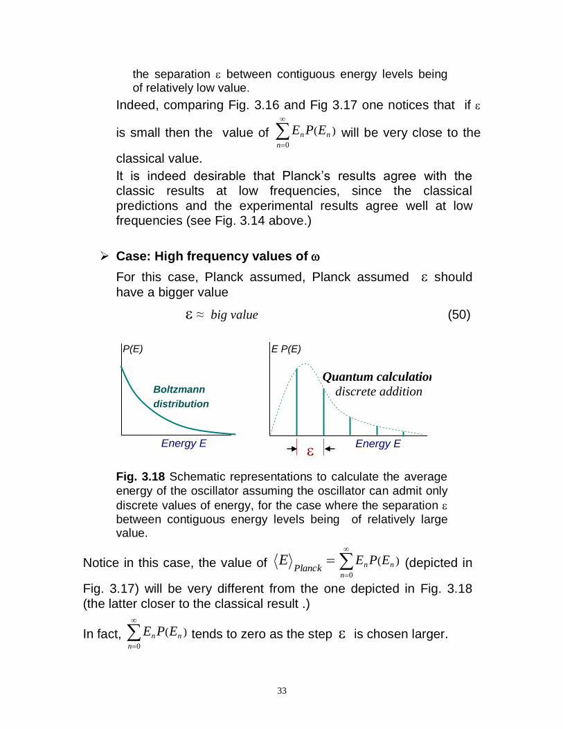
Case: High frequency values of

For this case, Planck assumed, Planck assumed should

have a bigger value

≈ big value (50)

Energy E

P(E)

Boltzmann

distribution

Energy E

E P(E)

<E>=

=Area

~kB T

Quantum calculation:

discrete addition

Fig. 3.18 Schematic representations to calculate the average

energy of the oscillator assuming the oscillator can admit only

discrete values of energy, for the case where the separation between contiguous energy levels being of relatively large value.

Notice in this case, the value of Planck

E )(

0

n

n

n EPE

(depicted in

Fig. 3.17) will be very different from the one depicted in Fig. 3.18 (the latter closer to the classical result .)

In fact, )(

0

n

n

n EPE

tends to zero as the step is chosen larger.

34

This result is desirable, since the experimental result indicate that

E tends to zero at high frequencies.

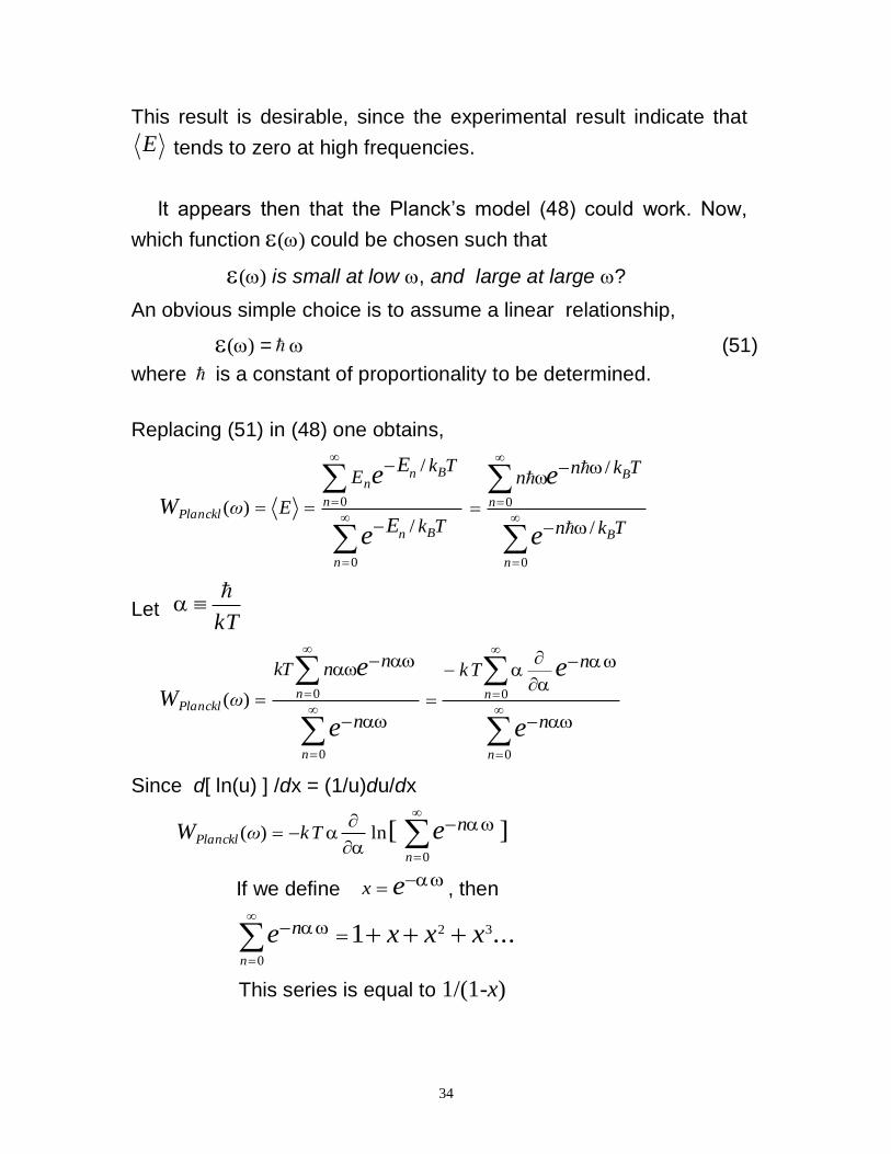
It appears then that the Planck‟s model (48) could work. Now,

which function () could be chosen such that

() is small at low , and large at large ?

An obvious simple choice is to assume a linear relationship,

() = (51)

where is a constant of proportionality to be determined.

Replacing (51) in (48) one obtains,

0

0

/

/

)(

n

Bn

Bn

n

n

PlancklTk

TkE

EωE

E

e

e

W

0

0

/

/

n

B

B

n

Tkn

Tknn

e

e

Let kT

0

0)(

n

nPlanckl

n

nnkT

ω

e

e

W

0

0

n

n

n

nTk

e

e

Since d[ ln(u) ] /dx = (1/u)du/dx

][ ln)(

0

n

PlancklnTkω eW

If we define ex , then

...1 32

0

xxxen

n

This series is equal to 1/(1-x)

35

= x1

1= 1

1

e

][][

0

1

1lnln)(

e

e TknTkω

n

PlancklW

][ 1ln

eTk

11

1

eee

TkTk

1

)(

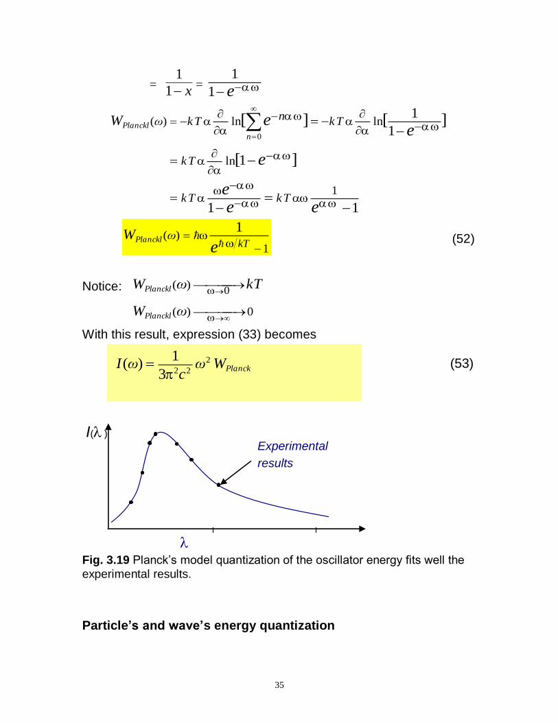
1

kTeωPlancklW

(52)

Notice: kTωWPlanckl 0

)(

0)(

ωWPlanckl

With this result, expression (33) becomes

PlanckWω

cωI

3

1)( 2

22 (53)

I()

Experimental

results

Fig. 3.19 Planck‟s model quantization of the oscillator energy fits well the

experimental results.

Particle’s and wave’s energy quantization

36

Historically. Planck initially (1900) postulated only that the energy of the oscillating particle (electrons in the walls of the blackbody) is quantized. The electromagnetic energy, once radiated, would spread as a continuous.

It was not until later that Plank accepted that the oscillating electromagnetic waves were themselves quantized. The latter hypothesis was introduced by Einstein (1905) in the context of explaining the photoelectric effect, which was corroborated later by Millikan (1914).

3.1.B.g Light Energy Density U() at equilibrium.

The Concept of Electromagnetic Modes

(see “Complement Chapter-3” notes (website)

3.2 PARTICLE-LIKE PROPERTIES of RADIATION

3.2.A Processes involving the absorption or scattering of radiation by particles

3.2.A.a Photoelectric effect Einstein‟s hypothesis of the quantized radiation energy

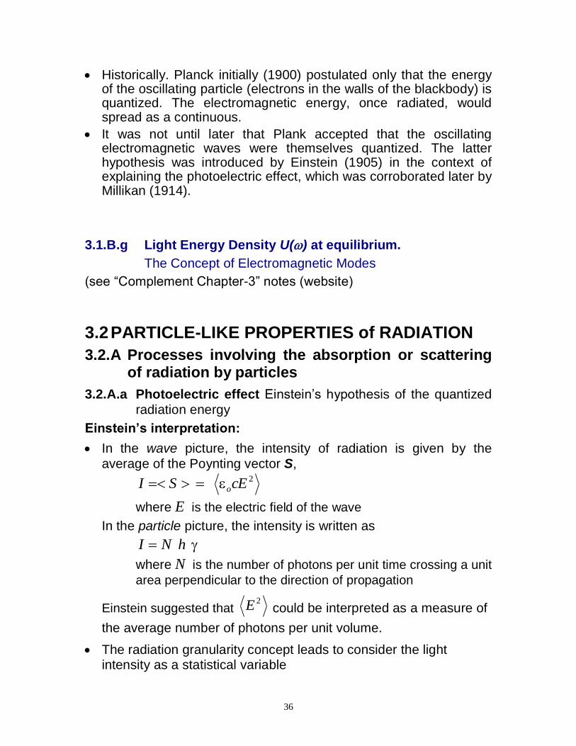
Einstein’s interpretation:

In the wave picture, the intensity of radiation is given by the average of the Poynting vector S,

2cESI o

where E is the electric field of the wave

In the particle picture, the intensity is written as

hNI

where N is the number of photons per unit time crossing a unit

area perpendicular to the direction of propagation

Einstein suggested that 2E could be interpreted as a measure of

the average number of photons per unit volume.

The radiation granularity concept leads to consider the light intensity as a statistical variable

37

A light source emits photons randomly in all directions

The exact number of photons crossing an area fluctuates (around an average number) in time and space

3.2.A.b The Compton Effect Scattering of a complete quantum of radiation in definite direction.

Compton explained the results on the assumptions that

each electron scatters a complete quantum of radiation (photon); and

the quanta of radiation are received from definite directions and are scattered in definite directions

3.3 WAVE-LIKE PROPERTIES of PARTICLES

3.3.A The Louis de Broglie Hypothesis

The Compton‟s Effect experiment had provided strong evidence on the particle nature of radiation. The typical symmetry expressed by Nature in many physical processes (for example, charges in motion produce magnetism and magnets in motion produce currents) may have led Louis de Broglie to propose the wave nature of particles.

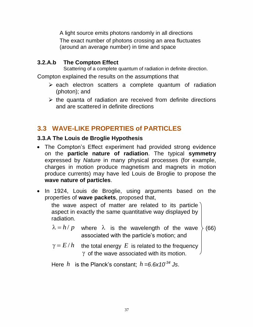
In 1924, Louis de Broglie, using arguments based on the properties of wave packets, proposed that,

(66)

the wave aspect of matter are related to its particle aspect in exactly the same quantitative way displayed by radiation.

ph / where is the wavelength of the wave

associated with the particle‟s motion; and

hE / the total energy E is related to the frequency

of the wave associated with its motion.

Here h is the Planck‟s constant; h =6.6x10-34 Js.

38

Since in the case of radiation )0( mmass we already know that

c , only one of the relationships above is needed to obtain

both and from its energy and momentum‟s particle properties.

In contrast, for a particle of mass 0m , one needs both

relationships given above to obtain the corresponding and .

Order of magnitude calculation of Brogliede

Case: m=10-3 Kg, v= 1 m/s p = mv = 10-3 Kg·m/s

=h/p = 6.6x 10-31 m. This value is inaccessible to any measurement currently possible

Case: me = electron‟s mass = 9.1x10-31 Kg, qe =1.6x10-19 C

If the electron accelerated through a potential difference of Vo volts its kinetic energy will be determined by

qe Vo =p2/2m, which gives 2/1)2( oee Vqmp

For Vo =50Volts: 2/1482/1 )1056.14()2( xVqmp oee

smxp /108.3 24

mxsmxsJxph 102434 07.1)/108.3/()106.6(/ .

This value is of the same order of magnitude of the X-rays‟ wavelength.

3.3.B Experimental confirmation of the de Broglie hypothesis. Electron Diffraction

In 1897 J. J. Thompson discovered the electron (establishing the ration qe / me. ) and was awarded the Nobel Prize in 1906.

The de Broglie wavelength Brogliede associated to an electron falls

in the order of Angstroms (when accelerated at moderate voltages ~ 50 Volts, as shown in the example above), which happens to be the inter-atomic spacing in a crystalline solid.

In 1926 Elsasser suggested that the wave nature of particles could

be tested by verifying whether or not electrons of the proper energy are diffracted by a crystalline solid.

39

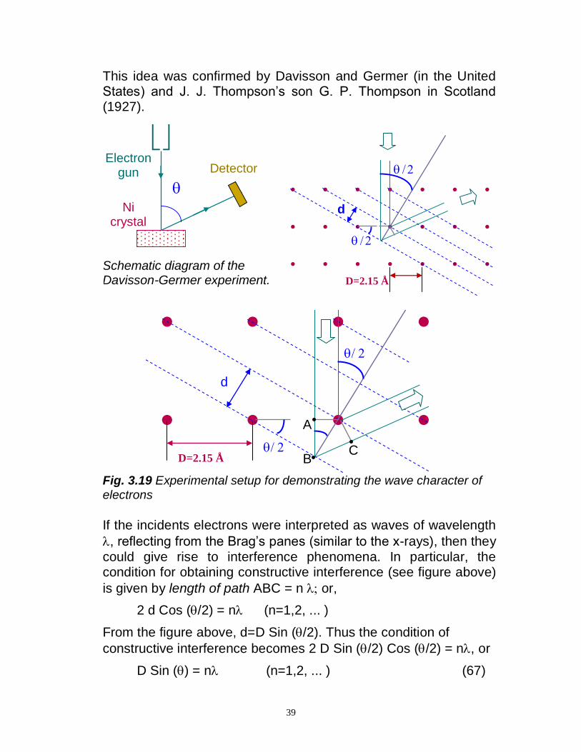
This idea was confirmed by Davisson and Germer (in the United States) and J. J. Thompson‟s son G. P. Thompson in Scotland (1927).

Electron gun Detector

Ni crystal

Schematic diagram of the Davisson-Germer experiment.

. . . . . . .

. . . . . . .

. . . . . . .

. . . . . . . D=2.15 Å

D=2.15 Å

d

. . . . . . .

. . . . . . .

. . . . . . . D=2.15 Å

d

A

B C

Fig. 3.19 Experimental setup for demonstrating the wave character of electrons

If the incidents electrons were interpreted as waves of wavelength

, reflecting from the Brag‟s panes (similar to the x-rays), then they could give rise to interference phenomena. In particular, the condition for obtaining constructive interference (see figure above)

is given by length of path ABC = n or,

2 d Cos (/2) = n (n=1,2, ... )

From the figure above, d=D Sin (/2). Thus the condition of

constructive interference becomes 2 D Sin (/2) Cos (/2) = n, or

D Sin () = n (n=1,2, ... ) (67)

40

For an accelerating voltage Vo = 54 volts, Brogliede

= h/p= 1.66 Å

(as calculated above). According to expression (46) it would be expected to observe a maximum of interference at,

Sin () = D

= degrees (theoretical prediction.)

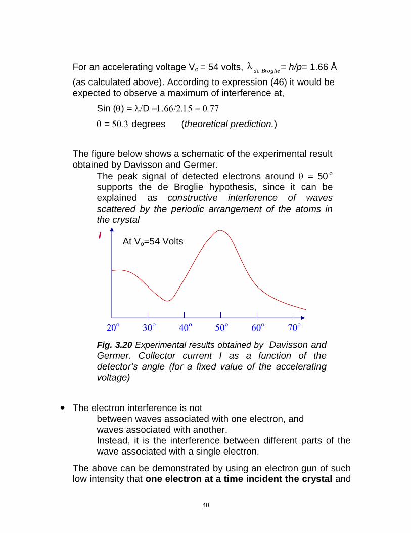
The figure below shows a schematic of the experimental result obtained by Davisson and Germer.

The peak signal of detected electrons around = 50 supports the de Broglie hypothesis, since it can be explained as constructive interference of waves

scattered by the periodic arrangement of the atoms in the crystal

I At Vo=54 Volts

Fig. 3.20 Experimental results obtained by Davisson and

Germer. Collector current I as a function of the detector’s angle (for a fixed value of the accelerating voltage)

The electron interference is not between waves associated with one electron, and waves associated with another. Instead, it is the interference between different parts of the wave associated with a single electron.

The above can be demonstrated by using an electron gun of such low intensity that one electron at a time incident the crystal and

41

by showing that the pattern of scattered electrons remains the same.

3.4 WAVE-PARTICLE DUALITY

Not only electrons but all materials, charge or uncharged, show wavelike characteristics:

Estermann, Stern, and Frish Molecular beams of hydrogen and atomic beams of helium

from a lithium fluoride crystal. The difficulties of these experiments lie in the low intensity of the molecular beams attainable.

Fermi. Marshall and Zinn Use the abundant slow neutrons available from nuclear

reactors. (X-ray analysis is based on the photon-electron interaction; neutrons rather interact with the nucleus.)

The particle aspect is emphasized when studying their emission

and detection

The wave aspect is emphasized when studying their motion

The small value of h impedes the observation of wave-particle duality in the macroscopic world.

Since ph / , a zero value for h would imply an absence of

diffraction effects. On the other hand, the (relatively) large momentum of macroscopic objects compared to h also makes

too small to be detected.

The deeper understanding of the link between the wave model and the particle model is provided by a probabilistic interpretation of the wave-particle duality:

In the case of radiation, it was Einstein who united the wave and particle theories (used in the explanation of the photoelectric effect.)

Max Born (many years after) applied later similar arguments to unite the wave and particle theories of matter. (Einstein, however, did not accept it.)

This latter aspect is more involved and becomes the subject of the next chapter.

42

_________________________

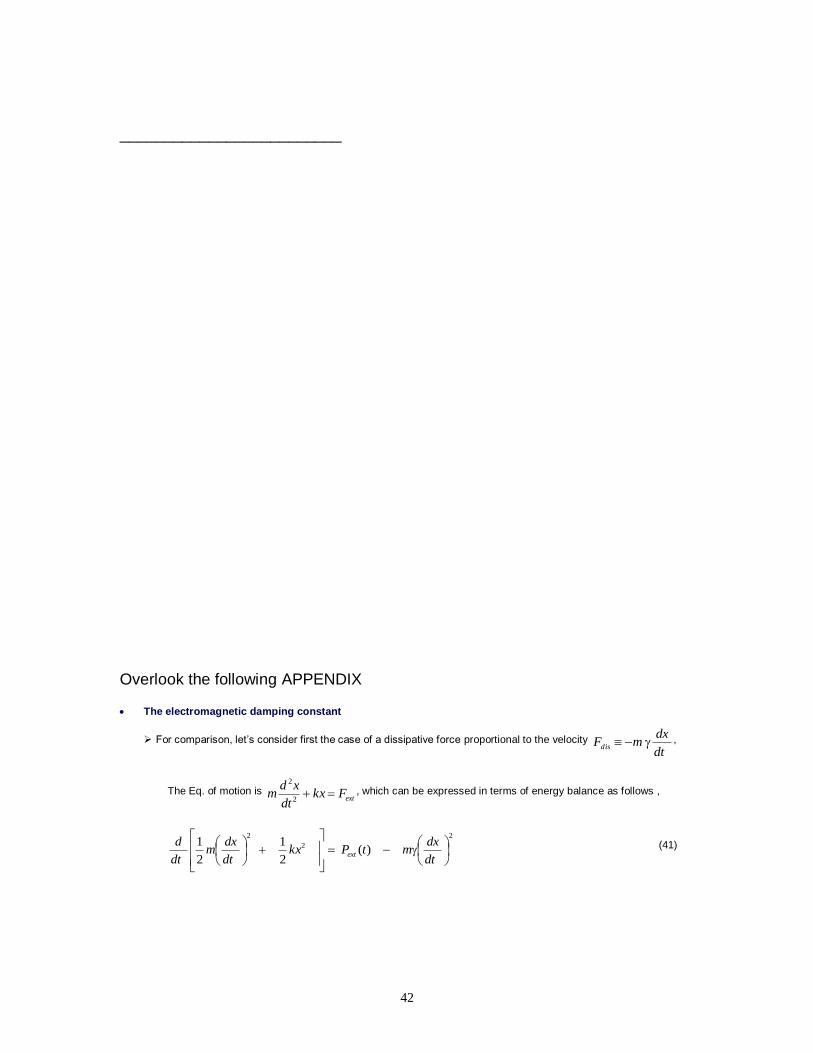
Overlook the following APPENDIX

The electromagnetic damping constant

For comparison, let‟s consider first the case of a dissipative force proportional to the velocity

dt

dxmFdis ,

The Eq. of motion is extFkx

dt

xdm

2

2

, which can be expressed in terms of energy balance as follows ,

2

2

2

)( 2

1

2

1

dt

dxmtPkx

dt

dxm

dt

dext

(41)

43

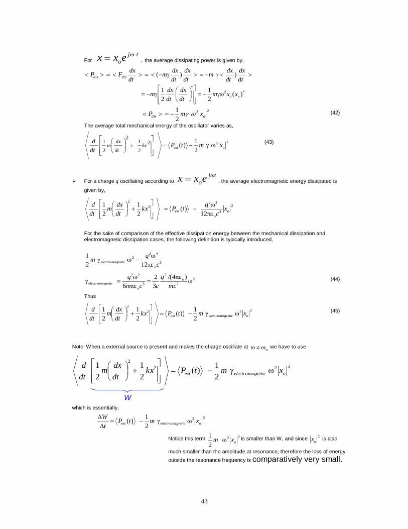
For tj

oexx , the average dissipating power is given by,

*2

*

)(2

1

2

1

))(

oo

disdis

xxmdt

dx

dt

dxm

dt

dx

dt

dxm

dt

dx

dt

dxm

dt

dxFP

22

2

1odis xmP (42)

The average total mechanical energy of the oscillator varies as,

22

2

1)(2

2

12

2

1oext xmtP

dt

dkx

dt

dxm

(43)

For a charge q oscillating according to tj

oexx , the average electromagnetic energy dissipated is

given by,

2

3

422

2

12)(

2

1

2

1o

o

ext xc

qtPkx

dt

dxm

dt

d

For the sake of comparison of the effective dissipation energy between the mechanical dissipation and electromagnetic dissipation cases, the following definition is typically introduced,

3

422

122

1

c

qm

o

neticelectromag

2

2

2

3

22 )4/(

3

2

6

mc

q

ccm

q o

o

neticelectromag (44)

Thus

222

2

2

1)(

2

1

2

1oneticelectromagext xmtPkx

dt

dxm

dt

d

(45)

Note: When a external source is present and makes the charge oscillate at o we have to use

222

2

2

1)(

2

1

2

1oneticelectromagext xmtPkx

dt

dxm

dt

d

W

which is essentially,

22

2

1)( oneticelectromagext xmtP

t

W

Notice this term 22

2

1oxm is smaller than W, and since

2

ox is also

much smaller than the amplitude at resonance, therefore the loss of energy

outside the resonance frequency is comparatively very small.

44

1 R. Eisberg and R. Resnick, “Quantum Physics,” 2nd Edition, Wiley, 1985. See Chapter

1 2 Feynman Lectures, Vol - I, Chapter 32