Chapter 3: INTERNALIZATION OF EXTERNALITIES

CHAPTER 3

1

Chapter 3: INTERNALIZATION OF EXTERNALITIES Contents 1. Bargaining solution 2. Price regulations (esp. taxes) 3. Quantity regulations 4. Evaluation of policy measures targeting prices and quantities 5. Environmental education 6. International measures and legal frameworks

1. Bargaining solution Concept: Up to the 1960s, it was a shared consensus between economists that externalities could only be internalized via government measures (e.g., taxes, subsidies, minimum or maximum prices, etc.). However, in 1961, R.H. Coase published his groundbreaking article “The Problem of Social Costs”, stating that government intervention is not the only way to internalize externalities. Rather, clearly defined and allocated property and usage rights are essential. The government has to provide the framework for negotiations between the actors by clearly allocating the property and usage rights for the public goods involved. Clearly allocated rights enable the actors to enter in negotiations. The Coase Theorem states that these negotiations lead to an efficient outcome, no matter which party had been allocated the original property and usage rights – as long as the government provides a legal framework including legal certainty and freedom of contract. There are basically two possibilities for the allocation of rights:

Model I: polluter-pays principle The property rights are allocated to the party who is (potentially) affected by pollution. I.e., the polluter has to pay a compensation to the property-rights holder if (and only if) he restricts the holder’s possibilities of production and/or consumption by causing an externality. Model II: affected-party-pays principle The property rights are allocated to the (potential) polluter. The (potentially) affected party compensates the polluter for avoiding the externality.

The outcome is the same in both cases: The optimal level of pollution is realised for both contracting parties, because financial transfers between parties are incorporating into their individual cost calculations. Hence, externalities are internalized. We speak of “potential” polluters and “potentially” affected parties because externalities may not even arise in this contractual setting. However: The distributional implications of different contractual forms of internalization are very different indeed; choosing a internalization procedure is, therefore, a political decision.

INTERNALIZATION OF EXTERNALITIES

2

Example: A cattle-farmer and a crop-farmer share a piece of soil for their respective production. However, the economic activity of the cattle-farmer limits the possibilities of production for the crop-farmer (since the cattle tramples down the crop), without this restriction being mirrored in market prices. There are two ways to internalize the damage: 1) polluter-pays principle: The property rights are allocated to the crop-farmer; the cattle-farmer compensates the crop-farmer for his loss in income. If the cattle-farmer anticipates his liability, he will possibly take precautions (such as building a fence) to prevent any damages to the crop-farmer. In that case the costs of those precautionary measures would internalize the externality. 2) affected-party-pays principle: The property rights are allocated to the cattle-farmer; the crop-farmer has to build a fence or compensate the cattle-farmer for holding less cattle. In this scenario the internalization of externalities prevents any effective damage, too. Critique of the Coase Model: Practical usability of the Coase Model is restricted due to the following reasons:

• Imperfect information: Are all affected parties involved in the negotiations? What are the “true” costs of damages and abatement, respectively? What is the “true” amount of compensation payments?

• Asymmetric information: Are all relevant information accessible and

ready for all concerned parties? What are the incentives for strategic behaviour? Can there still be an efficient outcome?

• Transaction costs: The costs of negotiation can be high, since the

negotiation process can be long and complicated. Furthermore, costs of controlling and enforcing any closed deal could arise.

• Negotiating power: The negotiating power of involved parties may

differ substantially. Hence the outcome may differ from an economically optimal result.

Due to the above criticisms, the practical relevance of the Coase model for any national environmental policy tends to be rather low. In this field, a stronger involvement of governmental measures seems sensible. However, as far as the solution of international or even global environmental problems is concerned, the Coase theorem still has its relevance. Take for example the problem of compensation payments from industrialized countries for developing countries in order to reduce emissions, especially CO2 emissions. Furthermore, emission certificates or so called “debt-for nature swaps” can be seen as concrete applications of the Coase Theorem. (These issues will be dealt with later in this chapter.)

CHAPTER 3

3

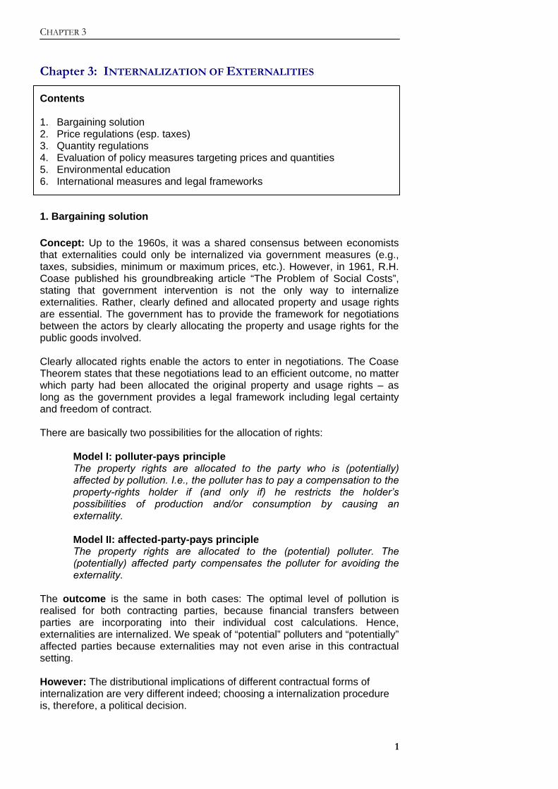
2 Price Regulation - taxation When dealing with externalities, we saw that the quantity x1 in figure 3.1, which is actually traded on the market, does not correspond to the quantity x2 which would be traded in the social optimum A. Figure 3.1 shows that quantity x2 is associated with a larger social benefit than quantity x1, the difference being x1x2BA. However, total social costs have increased by the even bigger amount x1x2CA; hence, ABC represents the net welfare loss due to externalities. These externalities have to be internalized to reach the socially optimal quantity.

Fig. 3.1:A Negative externality on the market

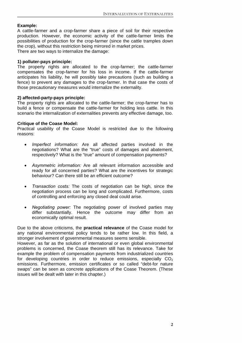
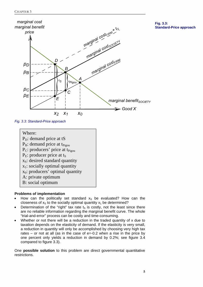
From the economist’s welfare perspective, the main question in the face of such an externality is how to motivate the firm to produce the socially optimal quantity of X. There are two ways to reach that goal by influencing the price of X, namely imposing a Pigou tax or the so called price-standard approach. 1. Pigou tax The concept of the Pigou tax was introduced by Arthur Cecil Pigou in his book “Economics of Welfare” (1920) and states that, in the case of complete information concerning the marginal benefits and – damages of firms and society, respectively, the socially optimal production of X can be reached by imposing a tax on X with a tax rate t which equals the difference between MCSociety and MCFirm for any amount of X produced. Thus: p1 = MCFirm(x1) + tax rate t(x1) = MCSocietyt(x1) The shaded area A in figure 3.2 shows the tax revenues for the government.

Fig. 3.1: A negative externality on the market


4

Fig. 3.2: Pigou-tax

The political and practical implementation of a Pigou tax, however, is very complex indeed, since all externalities have to be known and quantified in advance in order to determine the marginal costs to society and, hence, the tax rate. A complete record and monetary assessment of externalities is simply not possible (or at least very costly) at the present time, and that is why the difference between marginal costs for society and for the firm, respectively, cannot be accurately established. Hence, the Pigou tax cannot be implemented. One possible solution to this problem, however, is the so-called price-standard approach. 2. Standard-Price-approach Since the marginal costs of society and hence the optimal amount of X are not known precisely, one factor – in this case, the quantity of X – will be fixed as a “standard” (xS). xS should be as close as possible to the theoretically optimal (but unknown) quantity x1. Then, the tax rate tS is set to reach the market-clearing equilibrium at xS. If the resulting quantity (i.e. the quantity that is traded via the market at ts) corresponds to the standard quantity xS, tS was chosen “correctly”. If not, tS has to be adjusted in a process of “trial and error” to finally correspond to the standard quantity xS. This standard quantity, however, does not necessarily equal the socially optimal quantity, but is to be determined through the political process. The idea is exemplified in figure 3.3

Abb. 3.2: Pigou-tax

CHAPTER 3

5

Fig. 3.3: Standard-Price approach

Problems of implementation • How can the politically set standard xS be evaluated? How can the

closeness of xS to the socially optimal quantity x1 be determined? • Determination of the “right” tax rate tS is costly, not the least since there

are no reliable information regarding the marginal benefit curve. The whole “trial-and-error” process can be costly and time-consuming.

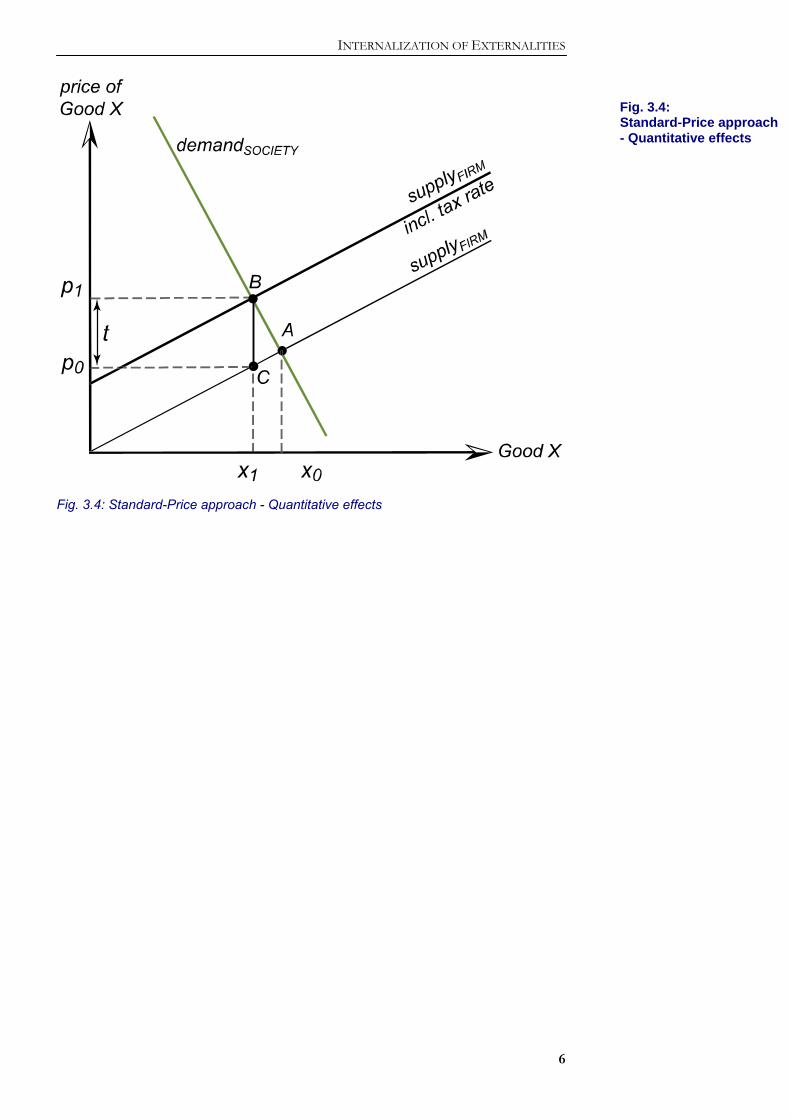
• Whether or not there will be a reduction in the traded quantity of x due to taxation depends on the elasticity of demand. If the elasticity is very small, a reduction in quantity will only be accomplished by choosing very high tax rates – or not at all (as in the case of e=-0.2 when a rise in the price by one percent only yields a reduction in demand by 0.2%; see figure 3.4 compared to figure 3.3).

One possible solution to this problem are direct governmental quantitative restrictions.

Where: PD: demand price at tS PB: demand price at tPigou PC: producers’ price at tPigou PE: producer price at tS xS: desired standard quantity x1: socially optimal quantity x0: producers’ optimal quantity A: private optimum B: social optimum

Fig. 3.3: Standard-Price approach


6

Fig. 3.4: Standard-Price approach - Quantitative effects

Fig. 3.4: Standard-Price approach - Quantitative effects

CHAPTER 3

7

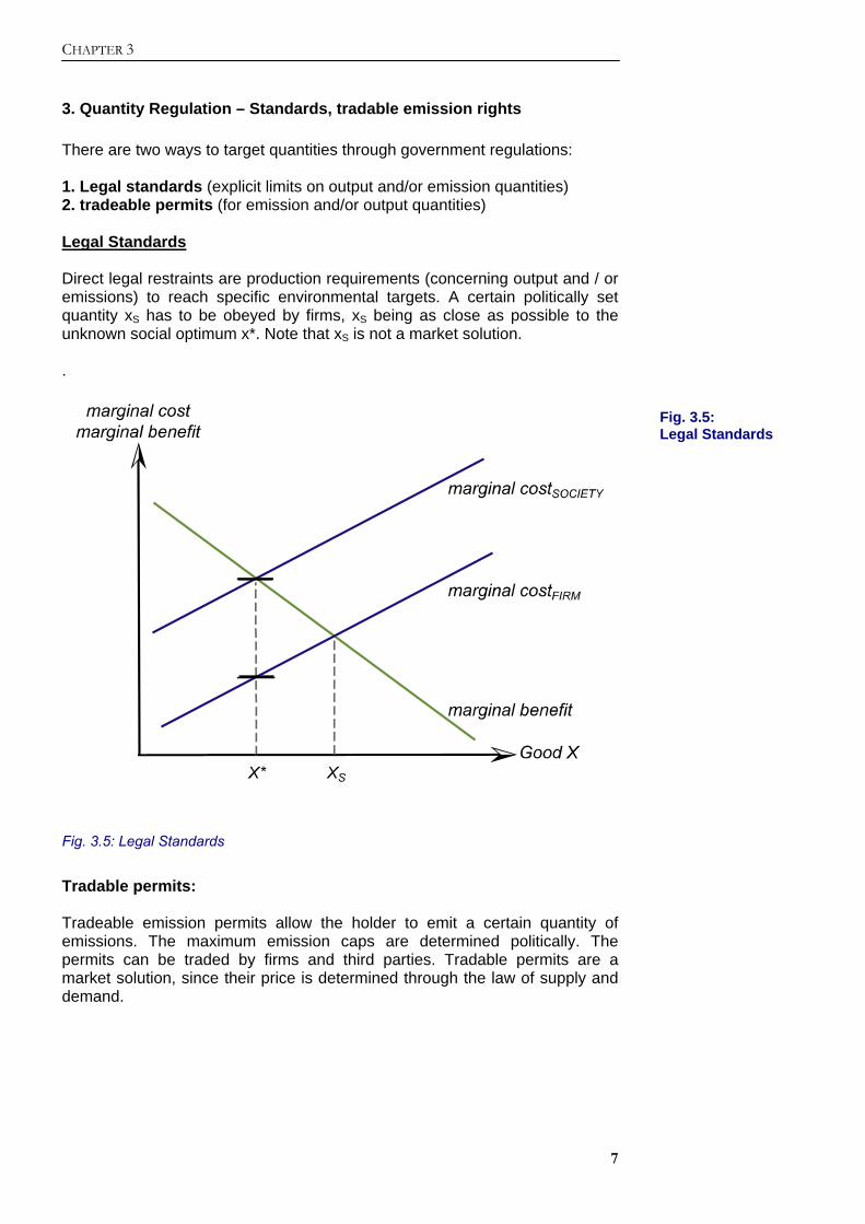
3. Quantity Regulation – Standards, tradable emission rights There are two ways to target quantities through government regulations: 1. Legal standards (explicit limits on output and/or emission quantities) 2. tradeable permits (for emission and/or output quantities) Legal Standards Direct legal restraints are production requirements (concerning output and / or emissions) to reach specific environmental targets. A certain politically set quantity xS has to be obeyed by firms, xS being as close as possible to the unknown social optimum x*. Note that xS is not a market solution. .

Fig. 3.5: Legal Standards

Tradable permits: Tradeable emission permits allow the holder to emit a certain quantity of emissions. The maximum emission caps are determined politically. The permits can be traded by firms and third parties. Tradable permits are a market solution, since their price is determined through the law of supply and demand.

Fig. 3.5: Legal Standards


8

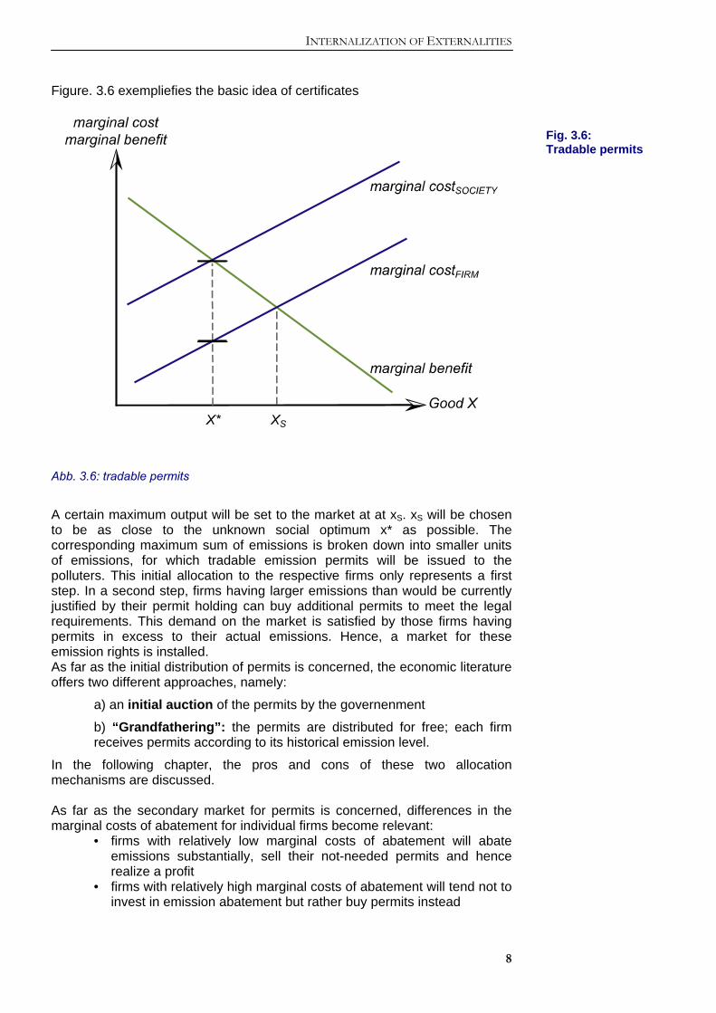
Figure. 3.6 exempliefies the basic idea of certificates

Abb. 3.6: tradable permits

A certain maximum output will be set to the market at at xS. xS will be chosen to be as close to the unknown social optimum x* as possible. The corresponding maximum sum of emissions is broken down into smaller units of emissions, for which tradable emission permits will be issued to the polluters. This initial allocation to the respective firms only represents a first step. In a second step, firms having larger emissions than would be currently justified by their permit holding can buy additional permits to meet the legal requirements. This demand on the market is satisfied by those firms having permits in excess to their actual emissions. Hence, a market for these emission rights is installed. As far as the initial distribution of permits is concerned, the economic literature offers two different approaches, namely:

a) an initial auction of the permits by the governenment

b) “Grandfathering”: the permits are distributed for free; each firm receives permits according to its historical emission level.

In the following chapter, the pros and cons of these two allocation mechanisms are discussed. As far as the secondary market for permits is concerned, differences in the marginal costs of abatement for individual firms become relevant:

• firms with relatively low marginal costs of abatement will abate emissions substantially, sell their not-needed permits and hence realize a profit

• firms with relatively high marginal costs of abatement will tend not to invest in emission abatement but rather buy permits instead

Fig. 3.6: Tradable permits

CHAPTER 3

9

4. Evaluation of policy measures targeting prices and quantities

1) An peliminary evaluation of tradable emission permits When evaluating permits, it is crucial to take into account how those permits are initially allocated to the different polluting entities, e.g. firms, single plants, or sectors. Auctioning of permits as a form of initial allocation Advantages of this allocation mechanism:

• Compared to attributing the permits “for free” (Grandfathering, see next section), an initial auction of permits is more efficient, since the right to produce emissions is associated with a price—reflecting its scarcity—right from the beginning of the schedule. If the market is sufficiently competitive, the initial price should equal firms’ marginal costs.

• Furthermore, an initial auction of permits is associated with higher dynamic incentive effects than “Grandfathering”, since in this case it pays for the firm to lower emissions even before permits are distributed. The dynamic incentive effects are considerably weaker in the case of “Grandfathering”; it is, moreover, even possible that firms strategically increase their emission levels right before the distribution of permits (see below).

• From a governmental point of view, an initial auction of permits can be attractive due to the associated additional revenue, if the permit system is not conceptualized as neutral to the government’s budget (neutrality can be achieved by simultaneous cuts on other sources of government funding, such as, for example, non-wage labour costs).

Problems associated with auctioning:

• An initial auction of permits favors those firms whose liquidity is high and who can, as a consequence, successfully bid on the initial auction.

• Secondly, an auction favors big firms (with substantial cash flow) over small ones, if the government does not assure budget neutrality of the permit system right from the beginning.


10

Free-of-charge distribution of permits (“Grandfathering”) Advantages of this allocation mechanism:

• Protection of the status quo: all existing firms get emission permits according to their past emission level free of charge. (But see “problems” below.)

• Grandfathering is comparatively easy to implement through the political process (“political feasibility”), since it is not associated with any initial costs to the firms and not associated with any increase in government revenues, which also increases the credibility of this model. (The same holds true for an initial auction of permits, however, if that auction is conducted in a way that ensures budget neutrality.)

Problems associated with a “free” initial allocation:

Grandfathering involves a risk of strategic behavior: Right before permits are attributed, firms have an incentive to increase emission levels in order to get a higher share of emission permits. To prevent this kind of reaction, the introduction and distribution of permits has to be executed as swiftly and efficiently as possible. Furthermore, the average past emission over several years should be taken as a reference point for the distribution schedule (instead of some fix year).

Problems related to both distribution schemes:

• Firms which intend to enter the market cannot get hold of any emission permits This potential complication can be solved by withholding a certain amount of permits and distribute them to newcomers if required.

• There is no guarantee that the marginal costs of abatement really

serve as a reference point for the allocation of permits (since the auctioning model favors the financially strong companies, and Grandfathering favors those with a high level of past emissions).

• Timing: Problems of timing include the choice of a closing date for the

schedule (this can be conceptualized either as a definite closing date for the right to produce emissions or as a step-by-step model which prescribes a reduction in emissions from year to year)

• Regional boundaries: The bigger the geographical spread of the

schedule, the better markets for permits will work (an unwanted consequence of the regional spread, however, might be the formation of local emission hot spots).

• Sectoral design: Which kinds of firms should be integrated in the

schedule? For example: Should only firms from the energy-producing sector be participating in the CO2-emission-trading?

No matter what kind of distributional model is chosen, there are two cornerstones of every scheme involving emission permits:

(1) actual emissions have to be verifiable

(2) the principle of legal certainty has to prevail That is to say the market for permits has to be ‘objectively’ controllable and the permits must be generally recognized. These conditions, however, imply that

CHAPTER 3

11

larger efforts on the level of administration and regulation of the market. Hence, the costs of implementation can be considerable. Examples for the permit trading The following two examples are chosen to illustrate the basic parameters that are crucial in determining the success or failure of a market for permits. In practical politics, an emission-permits scheme is often combined with emission standards, i.e., a certain emission level is set by law and any firm with emissions below that level gets emission credits for that difference. These emission credits can be traded and bought by those firms who due to their cost structure have to produce above the emission limit. Example 1: Emission-permit solution for nitrogen oxide and volative hydrocarbons in the region of Basle, Switzerland Introduced in 1991, this was only a short-lived scheme, since the market for permits was not working for the following reasons: emission standards were too strict, i.e., not enough emission credits on the market

1. 10%-clause: firms had to be below standards by at least ten percent to get emission credits

2. 80%-clause: only 80 percent of the revenues was credited to firms

3. a government agency had to autorise any usage of emission permits

4. no legal certainty: the period of validity of permits was unknown

Example 2: SO2-permits in the United States

Introduced in 1995 as part of the US-acid-rain program, the objective of the SO2-permits was a reduction of SO2-Emissions by 10 percent below the level of 1980 (by 2010). There were 20 million permits on the market in 2000. Strict sanctions (penalties) guarantee an efficient functioning of the market for permits. If the legally set emission standard is violated, penalties of $2000/ton of SO2 are due (the price per permit is $200/ton of SO2).

• Compared to the preceding situation with politically set emission standards, the firms’ costs to reduce emissions sunk by approximately 42 percent.

• By reducing the maximum emission level each year, the government creates a dynamic incentive for emission reduction which leads to an average decrease of 25 percent in SO2-emissions compared to fix standards.


12

2) Factors for an appraisal of environmental policies To evaluate and compare different environmental policy instruments, the following criteria have to be considered:

a) Ecological effectiveness: Is the instrument suited to reach a given environmental policy target (such as, for example, a certain predetermined reduction in emissions)?

b) Economic efficiency: Is the environmental policy target reached with a minimum of total costs to society?

c) Costs of implementation: Which instrument is associated with the lowest administrative costs?

d) Dynamic incentive effects: Are incentives set to further reduce externalities in the future? Are incentives set to promote technological change?

3) Evaluating tax solutions versus emission standards by criteria a-d

a) Ecological effectiveness Emission standards are ecologically highly effective, since any politically desired emission level can be directly enforced by law. In this sense, emission standards are more efficient than taxes. The elasticity of demand may be so low that even very high taxes will not introduce any substantial reduction in consumption or emissions, respectively. Furthermore, since the slope of the firms’ marginal costs of abatement (MCA) is not precisely known, the tax rate t has to be determined by a trial-and-error procedure. The probability of finding the ecologically “right” tax rate right at the beginning of this process is, needless to say, very low.

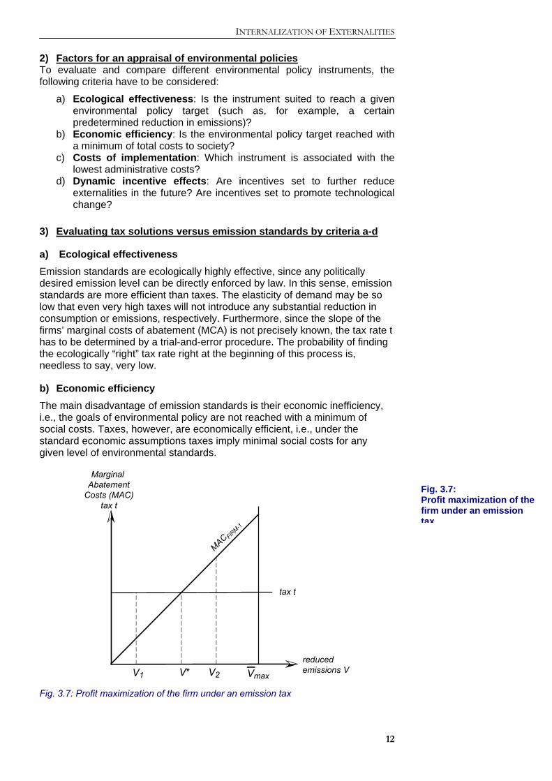
b) Economic efficiency The main disadvantage of emission standards is their economic inefficiency, i.e., the goals of environmental policy are not reached with a minimum of social costs. Taxes, however, are economically efficient, i.e., under the standard economic assumptions taxes imply minimal social costs for any given level of environmental standards.

reducedemissions VV2

MarginalAbatement

Costs (MAC)tax t

V*

MAC FIRM-1

tax t

V1 Vmax Fig. 3.7: Profit maximization of the firm under an emission tax

Fig. 3.7: Profit maximization of the firm under an emission tax

CHAPTER 3

13

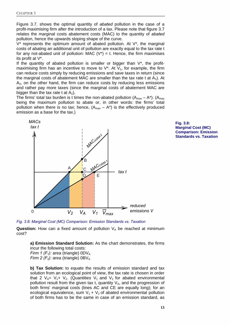
Figure 3.7. shows the optimal quantity of abated pollution in the case of a profit-maximising firm after the introduction of a tax. Please note that figure 3.7 relates the marginal costs abatement costs (MAC) to the quantity of abated pollution, hence the upwards sloping shape of the curve. V* represents the optimum amount of abated pollution. At V*, the marginal costs of abating an additional unit of pollution are exactly equal to the tax rate t for any not-abated unit of pollution: MAC (V*) = t. Hence, the firm maximises its profit at V*. If the quantity of abated pollution is smaller or bigger than V*, the profit-maximising firm has an incentive to move to V*. At V1, for example, the firm can reduce costs simply by reducing emissions and save taxes in return (since the marginal costs of abatement MAC are smaller than the tax rate t at A1). At A2, on the other hand, the firm can reduce costs by reducing less emissions and rather pay more taxes (since the marginal costs of abatement MAC are bigger than the tax rate t at A2). The firms’ total tax burden is t times the non-abated pollution (Amax – A*). (Amax being the maximum pollution to abate or, in other words: the firms’ total pollution when there is no tax; hence, (Amax – A*) is the effectively produced emission as a base for the tax.)

reducedemissions VV2

MACstax t

MAC FIRM-2

tax t

V1 Vmax

MACFIRM-1

0

A

B

CD E

VA Fig. 3.8: Marginal Cost (MC) Comparison: Emission Standards vs. Taxation

Question: How can a fixed amount of pollution VA be reached at minimum cost?

a) Emission Standard Solution: As the chart demonstrates, the firms incur the following total costs: Firm 1 (F1): area (triangle) 0DVA Firm 2 (F2): area (triangle) 0BVA

b) Tax Solution: to equate the results of emission standard and tax solution from an ecological point of view, the tax rate is chosen in order that 2 VA= V1+ V2. (Quantities V1 and V2 for abated environmental pollution result from the given tax t, quantity VA, and the progression of both firms’ marginal costs (lines AC and CE are equally long); for an ecological equivalence, sum V1 + V2 of abated environmental pollution of both firms has to be the same in case of an emission standard, as

Fig. 3.8: Marginal Cost (MC) Comparison: Emission Standards vs. Taxation


14

well as in case of a tax solution and equals 2 VA, since all firms abate the amount VA in case of the emission standard solution.) Firm 1: F1 chooses V1, which causes costs corresponding to area (triangle) 0EV1. Area VADEV1 represents the additional costs compared to the costs occurring in case of the emission standard solution for firm 1. Firm 2: F2 chooses V2, which causes costs corresponding to area (triangle) 0AV2. Area V2ABVA represents the cost effectiveness compared to the costs occurring in case of the emission standard solution for firm 2.

In order to compare emission standard and tax solution, area VADEV1 and area V2ABVA will now be considered. The additional costs occurring for firm 1 (VADEV1) are lower than the cost efficiency for firm 2 (V2ABVA). In case of an emission standard, the total costs are higher than in case of taxation (plus areas ABC + CDE). Conclusion: The total costs are lower in the case of a tax solution than in the case of an emission standard solution. The efficiency advantage of the tax solution depends on whether the tax takes into account the differences in the marginal costs of abatement. If not all firms abate the same amount of emissions, but firms with low marginal costs abate much, and firms with high marginal costs abate little, the total costs of a given abatement are especially low.

c) Costs of Implementation Incurring costs for the implementation and maintenance of environmental policy targets through emission standards or taxes are similar for both solutions: Costs of Control (are emission standards complied with, or are taxes paid?):

Costs of Control (Emission Standards) ≈ Costs of Control (Taxes) Sanction Costs (penalties in case of non-compliance, or non-payment of taxes):

Sanction Costs (Emission Standards) ≈ Sanction Costs (Taxes) Costs of the determination of VA or t:

Legal standards are slightly more preferable than taxation with respect to these costs, because for the determination of t, the process of trial-and-error can be more costly and time consuming.

Conclusion: No significant differences exist between the costs of implementation of emission standards and taxes.

d) Dynamic Incentive Effects Emission Standards provide certain incentives for environmental technological advances. New environmental policies reduce costs, because previous environmental policy targets can be achieved at lower cost today (thanks to new technologies, such as better filters). Taxes can give fundamental dynamic incentives, too. All technological improvements lower taxes payable for the previous quantity of abatement. As demonstrated below, the net savings resulting from more emissions

CHAPTER 3

15

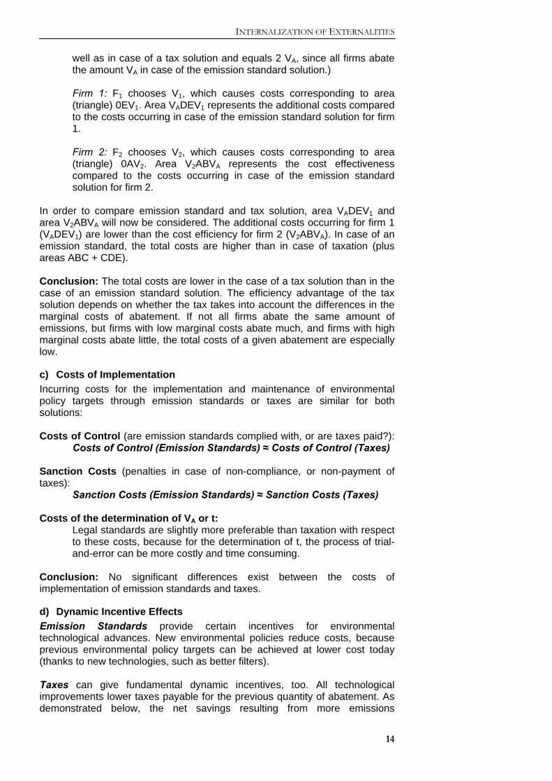
abatement will be positive in each case, and in total higher than in case of an emission standard. In case of taxation, as well as emission standards, the reduction of costs due to environmental technological progress is in fact opposed to additional costs caused by abatement efforts (e.g. purchase or development of new filter units). A firm is only interested in reducing the quantity of pollution, if the reduction in cost is higher than the costs resulting from the development and implementation of reduction measures. In general, firms are not interested in the development and implementation of new technologies, should the government plan to implement stricter emission standards. There is even the concern that technological innovations are held back in order to prevent the government from implementing stricter emission standards and adapting them to new technologies (“The Chief Engineers’ Cartel of Silence”). Whether emission standard or the tax solution provide an incentive to reduce costs by means of technological advances is demonstrated in the following charts (fig. 3.9 and 3.10): 1. Emission Standard Solution:

reducedemissions V

MACstax t

MAC FIRM-1

V’A Vmax

MAC’ FIRM-1

0

FH

VA Fig. 3.9: Dynamic Incentive Effects – Emission Standards

Implementing new technologies causes a shift of the marginal cost curve from MACFirm1 to MAC'Firm1 (the abatement becomes cheaper in total). Thus, a reduction in costs corresponding to area F is created. Technological innovations are created if the cost effectiveness F that is reached over a period of time is higher than the costs a firm would incur for the development and implementation of new technologies. If the government responds to technological changes by means of stricter standards (VA → V'A), the firms incur additional costs as high as corresponding to area H. The net gain resulting from technological improvements now only equals F-H and can be zero or even negative. The firms therefore have an incentive not to use the cheapest abatement technology in case of a legal standard; technological possibilities are often even consciously concealed (“The Chief Engineers’ Cartel of Silence“).

Fig. 3.9: Dynamic Incentive Effects – Emission Standards


16

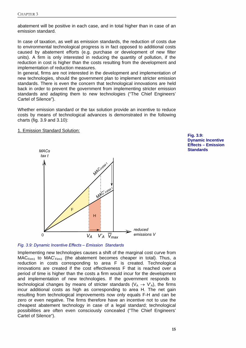
2. Tax Solution:

reducedemissions VV*

MACstax t

MAC FIRM-1

tax t

V*’ Vmax

MACFIRM-1

0

K

H

F


Implementing new technologies causes a shift of the marginal cost curve from MACFirm1 to MAC'Firm1. Costs corresponding to area F can be reduced for quantity V*. Due to the shift of the marginal costs of abatement, V* is not the optimal quantity anymore. Instead, the firm can profit by raise the abatement units to V*'. Thus, additional abatement costs corresponding to H incur. Considering the lower taxes for the firm in case of V*' ((Vmax - V*’)·t instead of (Vmax - V*)·t), there is a net gain corresponding to area K remaining through the shift from V* to V*'. In case of taxation, sum F+K is bigger than in case of an emission standard, which makes the tax solution more preferable. Conclusion: Taxes, as well as emission standards, provide fundamental incentives for environmentally friendly technological advances. Those incentives are not effective though, if firms speculate on an increase of standardized quantities or of tax rates due to the firms’ reductions in expenses. Taxes generate the strongest incentive for implementing environmentally friendly technologies.


CHAPTER 3

17

4) Summary: Applicability in Comparison “Permits (P) vs. Standards (S)

vs. Taxes (T)“ • Cumulative Comparison: Criteria a)-d)

a) Ecological Effectiveness ecological eff.(P) ≈ ecological eff.(S) > ecological eff.(T)

b) Economic Efficiency (Pareto Efficiency) economic eff.(P) ≈ economic eff.(T) > economic eff.(S)

c) Costs of Implementation Costs of implementation(T) ≈ costs of implementation(S) ≈ costs of implementation(P)

d) Dynamic Incentive Effects dyn. incentive(P) ≈ dyn. incentive(T) > dyn. incentive(S)

Taxation and emission standards both create fundamental incentives for environmentally friendly technological renewals. But taxes provide a stronger incentive for the implementation of these technologies than do emission standards. If the permit markets are functioning, there is also an incentive for technological improvements in case of tradable permits. In this case, the tradable permit solution is equally advantageous as the tax solution (additional profits). In general, incentive mechanisms do not become effective if it is speculated that the firms’ savings result in the government increasing standardized emissions levels or tax rates.

• Cumulative Comparison: Applicability of taxes, emission standards,

and tradable permits in terms of environmental policy - Emission Standards as environmental policy instruments make sense

if ecological effectiveness is valued or if it is probable that the demand curve is inelastic (ε very small).

- Taxes as environmental policy instruments make sense if economic efficiency is the main concern, if incentive mechanisms for the creation of environmentally friendly technologies ought to be strong, or if it is known that the elasticity of demand is rather high.

- Tradable Permits can be beneficial in connecting the advantages of emission standards (ecological effectiveness) and taxation (economic efficiency, dynamic incentive effects), if the permit markets are functioning. In that case, tradable permits are the best available environmental policy instrument.

Despite the many advantages of the tradable permit solution, studies have proven that in practice, the majority of solutions are emission standards. The reason for this circumstance is that the implementation of emission standards is more advantageous for certain groups (e.g. politicians, the bureaucracy, or other groups of interest) and therefore more supported by them through lobbying (see chapter 5).


18

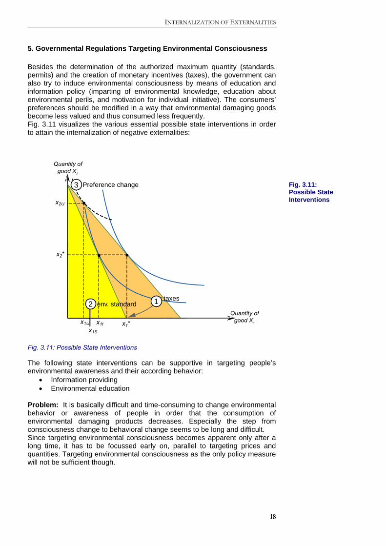
5. Governmental Regulations Targeting Environmental Consciousness Besides the determination of the authorized maximum quantity (standards, permits) and the creation of monetary incentives (taxes), the government can also try to induce environmental consciousness by means of education and information policy (imparting of environmental knowledge, education about environmental perils, and motivation for individual initiative). The consumers’ preferences should be modified in a way that environmental damaging goods become less valued and thus consumed less frequently. Fig. 3.11 visualizes the various essential possible state interventions in order to attain the internalization of negative externalities:

Quantity ofgood X1

Quantity ofgood X2

x1S

x1t

env. standard

Preference change

x2*

x2U

x1*

a

3

2 1

x1U

taxes

Fig. 3.11: Possible State Interventions The following state interventions can be supportive in targeting people’s environmental awareness and their according behavior:

• Information providing • Environmental education

Problem: It is basically difficult and time-consuming to change environmental behavior or awareness of people in order that the consumption of environmental damaging products decreases. Especially the step from consciousness change to behavioral change seems to be long and difficult. Since targeting environmental consciousness becomes apparent only after a long time, it has to be focussed early on, parallel to targeting prices and quantities. Targeting environmental consciousness as the only policy measure will not be sufficient though.

Fig. 3.11: Possible State Interventions

CHAPTER 3

19

6. International Measures and Legal Framework In this paragraph, our previous discussion is transferred to the international level: The internalization of externalities is now applied to global environmental problems. Basic Problems: The actors are subject to various domestic political and institutional regulations. There is no superior “supranational” institution holding the monopoly of legitimate use of force and capable to define and enforce the property rights for environmental goods. Possibilities for the Internalization of Global Externalities in the Environmental Context: 1. Trade Restrictions as a reaction to the cause of negative externalities

Concept: Countries causing negative externalities should be “penalized” with importation restrictions from other countries. Restraints of trade are not completely approved of due to the following reasons: - Trade restrictions can have excessive consequences for the people - It is difficult to conclusively determine who is responsible for the

externalities (producing, or consuming countries) - There is the issue about who has the power to sanction other countries

with trade restrictions. - Trade restrictions are hard to enforce and rather inefficient. At this point, we should refer to the so-called eco-labels. Eco-labels are voluntary environmental policy instruments. The consumer is provided a transparent statement about the relative environmental compatibility of the labelled product. Such labels can indirectely represent trade restrictions.

2. International Treaties

Only a few successful environmental conventions have been contracted to date. There are regional and global conventions. Basically, it pertains: The smaller the number of participants, the more intense the relation between the conventional partners; and the more directly they are concerned, the less significant cooperative problems are (compare the Prisoner’s Dilemma; see previous chapter). The cost-benefit-perspective of the respective countries is decisive for the success of an international environmental convention.


20

Examples:

- Regional Treaties:

a) September 1983: Convention between Germany, Belgium, Denmark, the European Community, France, Great Britain, the Netherlands, Norway, and Sweden regulating the collaboration in the prevention of the pollution of the North Sea by oil and other pollutants.

b) June 1994: Convention between Bulgaria, Germany, Croatia, Austria, Rumania, the Slovak Republic, Slovenia, the Czech Republic, Ukraine, and Hungary regulating the collaboration in the protection and environmentally compliant use of the Danube river.

- Global Treaties:

a) The Montreal Protocol, signed in October 1997: effective since January 1998: signed by 29 countries and the former EC. The protocol and its additional agreement regulated the phasing out of CFCs (chlorofluro carbons). Since January 1st 1996, their production is completely banned in all industrial countries. Developing countries were given a transition period until 2010. The discovery of an only slightly more expensive substitute for CFCs before the protocol had entered into force is decisive for its success. b) The Kyoto Protocol, December 1997: To date, 55 countries have ratified the protocol. The Kyoto Protocol aspires to reduce global emissions by 5 percent by the year 2012, below the level of emissions of 1990. The respective countries have determined individual values: The EU targets to reduce emissions by 8 percent as a whole (with varying values among the member countries), the United States by 7 percent, and Switzerland binds itself to reduce emissions by 8 percent. The Kyoto Protocol hit the headlines in the beginning of April 2001, when newly-elected US President George W. Bush Jr. refused to apply the agreement. The Kyoto Protocol is only realized if 55 of the countries discharging the highest quantity of CO2 emissions have signed it. The joining of Japan in May 2002 has been an important step. The ratification is now depending on Russia. It is presently very probable that also Russia will join the protocol.

3. Conditionality

Concept: Connecting financial transfers with conditions regarding content. Example: Debt-for-Nature-Swaps The first swap occurred between the environmental organization "Conservation International" and the Bolivian government in 1987. Proceeding: An environmental organization buys a certain debt from a country X for a price that lies below the nominal value of the debt (converted into the respective currency) on the secondary market of a creditor bank, in order to invest in environmental projects.

CHAPTER 3

21

Problems: - Environmental organizations have only limited purchasing power - Short supply on secondary markets ("moral hazard" caused by

governmental support measures for creditor banks) - Bare sustainability of those environmental projects - Inflation peril in the developing country → Solution: grading the

financial investment or national debt.

4. International transfer and compensation payments

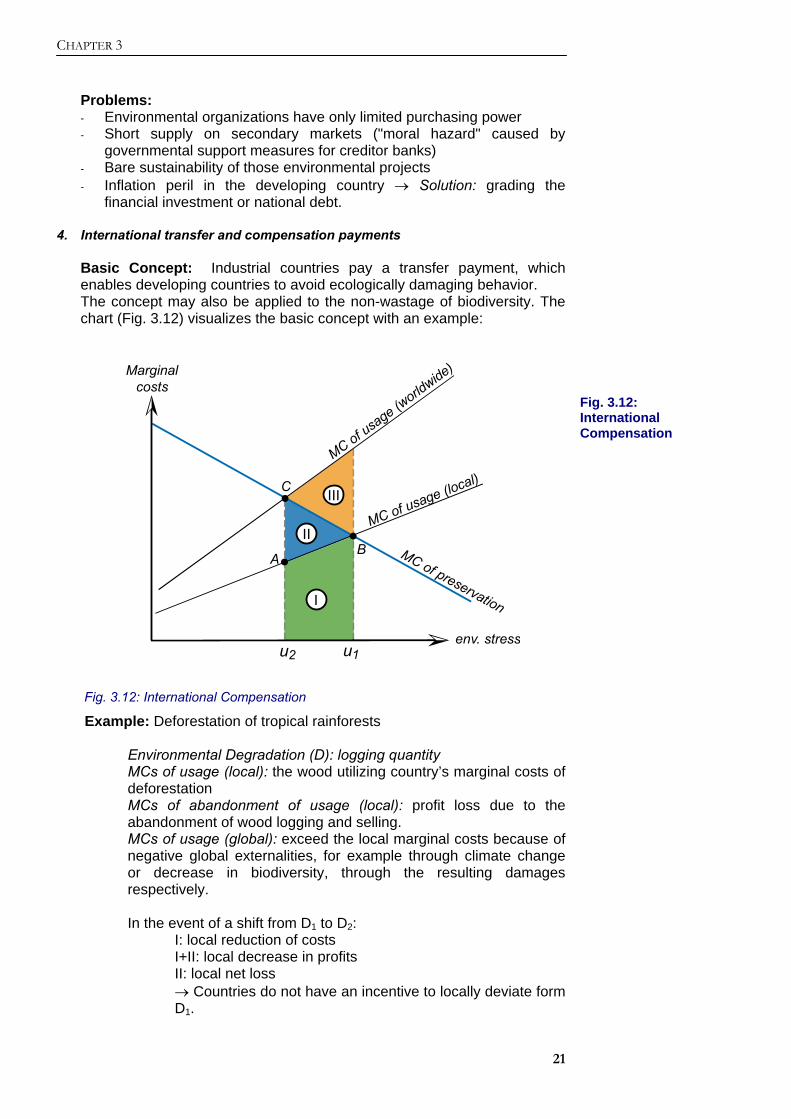
Basic Concept: Industrial countries pay a transfer payment, which enables developing countries to avoid ecologically damaging behavior. The concept may also be applied to the non-wastage of biodiversity. The chart (Fig. 3.12) visualizes the basic concept with an example:

env. stressu2

Marginalcosts

MC of usage (w

orldwide)

u1

B

C

MC of preservation

A

MC of usage (local)

I

II

III

Fig. 3.12: International Compensation

Example: Deforestation of tropical rainforests

Environmental Degradation (D): logging quantity MCs of usage (local): the wood utilizing country’s marginal costs of deforestation MCs of abandonment of usage (local): profit loss due to the abandonment of wood logging and selling. MCs of usage (global): exceed the local marginal costs because of negative global externalities, for example through climate change or decrease in biodiversity, through the resulting damages respectively. In the event of a shift from D1 to D2:

I: local reduction of costs I+II: local decrease in profits II: local net loss → Countries do not have an incentive to locally deviate form D1.

Fig. 3.12: International Compensation


22

→ In order to create an incentive to transit from D1 to D2 for rainforest countries, their net loss has to be compensated.

As highlighted below, there is potential for that:

III + II + I: global reduction of costs III (area CBD): global net gain

→ Global net gain (CBD) can be used to compensate the local net loss (ABC).

Problem of this solution: Such compensations are seldom paid because of the following difficulties in practical application: - Coordination/ distribution problems in providing and receiving countries - Insufficient knowledge about the amount of compensation (global/ local

marginal costs of degradation unknown or hardly determinable) - Application failure on the basis (e.g. who compensates for the

woodcutter’s daily wages?). Compensations are first paid to the respective governments.

5. “Joint Implementation and the Clean Development Mechanism“

CO2 emissions pose a global environmental problem. The location, where CO2 is emitted, absorbed, or reduced, is insignificant for the resulting climate effects. In the Rio Conference of 1992, it was decided to work out an internationally coordinated procedure in order to reduce CO2 emissions. This was adhered in the Kyoto protocol on climate change of 1997. Three groups of countries have been distinguished: AnnexB-Countries: These countries are obliged to sink their greenhouse gases between 2008 and 2012 to at least 8% below their 1990 level. Exceptional cases: To motivate important, but countries with a critical attitude towards the protocol, the emissions level has been alleviated for them: USA, Canada, Russia, 5% under the level of 1990 each, Japan 4.5%. Developing Countries (DCs): These countries do not have to reduce their emissions, but maintain their current level (no reduction obligation). Observations: There are major technological differences between the individual countries. Former Eastern bloc countries can reduce CO2 emissions relatively easily and at low cost, while western European countries are already working with technologies “producing“ a small amount of emissions. A further reduction is therefore only attainable at relatively high additional cost. Hence, the countries have different marginal costs of abatement (MCA), of which we have learned their typical curve sloping in the above chart. This is where the concept of Joint Implementation assails: Countries comply with common duties in order to globally reduce CO2 emissions at minimum cost. This idea follows the mechanism that we have learned above, saying that the total costs of abatement are only minimized if the marginal costs of abatement are equal everywhere, or in other words, if countries with (originally) high marginal costs of abatement abate a rather small quantity, and countries with (originally) low marginal costs of

CHAPTER 3

23

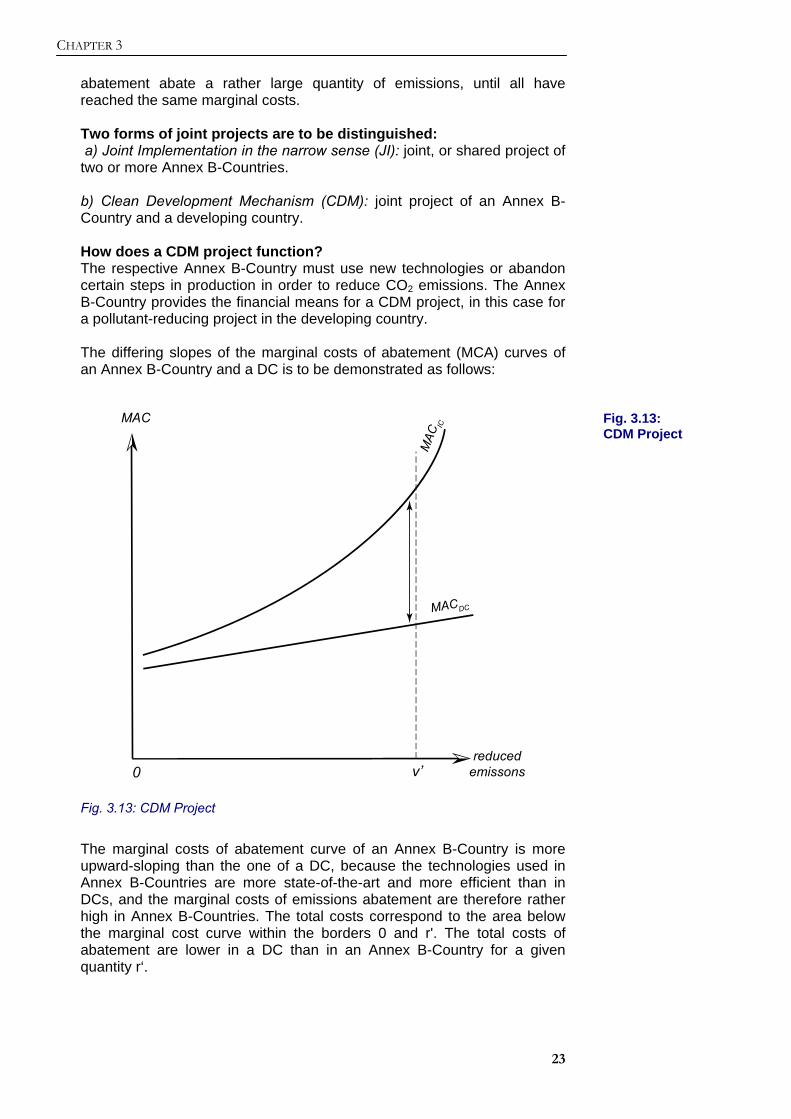
abatement abate a rather large quantity of emissions, until all have reached the same marginal costs. Two forms of joint projects are to be distinguished: a) Joint Implementation in the narrow sense (JI): joint, or shared project of two or more Annex B-Countries. b) Clean Development Mechanism (CDM): joint project of an Annex B-Country and a developing country. How does a CDM project function? The respective Annex B-Country must use new technologies or abandon certain steps in production in order to reduce CO2 emissions. The Annex B-Country provides the financial means for a CDM project, in this case for a pollutant-reducing project in the developing country. The differing slopes of the marginal costs of abatement (MCA) curves of an Annex B-Country and a DC is to be demonstrated as follows:

reducedemissons

MAC

0 v’

MACDC

MAC

IC

Fig. 3.13: CDM Project

The marginal costs of abatement curve of an Annex B-Country is more upward-sloping than the one of a DC, because the technologies used in Annex B-Countries are more state-of-the-art and more efficient than in DCs, and the marginal costs of emissions abatement are therefore rather high in Annex B-Countries. The total costs correspond to the area below the marginal cost curve within the borders 0 and r'. The total costs of abatement are lower in a DC than in an Annex B-Country for a given quantity r‘.

Fig. 3.13: CDM Project


24

Empiricism: There are currently approximately 180 ongoing CDM projects, of which many are afforestation projects, power plants, cement factories, and solar projects. Remarks: The pressure to effectuate JI or CDM projects has been decreasing since CO2 sinkers (e.g. forests) have been commonly acknowledged as a measure to reduce CO2. The following questions arose during practical application: • Are the projects conducted additional to, or instead of development

cooperation projects? • How are reductions measured? In other words, is the old power plants

in a DC withdrawn from the grid after a new one is constructed? • What counts as a reduction and in which case (reference point)? • Who conducts the measurements? • Monitoring: How are low emissions monitored on the long-term (how

good is the management and maintenance after the construction)? How often are emissions to be measured? Who conducts those measurements?

• Abatement Credits: How are the abated emissions to be split between Annex B-Country and DC? Credit for a reduction possibly provides an incentive for the DC to manage and maintain well the facilities in the future. May an Annex B-Country completely fulfil its duties through CDM projects (moral argument; no new environmental technologies in the Annex B-Country itself)?

• Follow-Up Costs: Who finances the education costs for the staff; who finances working expenses in CDM projects?

A summary of the pros and cons of the Clean Development Mechanism (CDM): Pros: A given CO2 reduction can be reached economically efficiently, especially Annex B-Countries benefit directly; there is potential of compensation for DCs. Complimentary resource and technology transfer to DCs. Cons: (Possible) decline in funds for development cooperation. Cheap reduction potentials are not available to DCs anymore, due to an exhaustion caused by AnnexB-Countries (solution: the AnnexB-Country pays a compensation from its efficiency gain; DC receives credit for the emission reduction). Possible delay in the development of environmentally friendly technologies.

CHAPTER 3

25

6. Repetition: National environmental policy, however applied to global

environmental problems

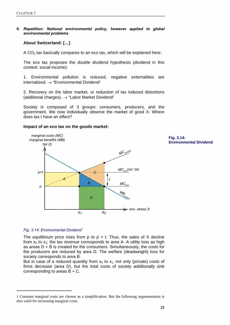
About Switzerland: […] A CO2 tax basically compares to an eco tax, which will be explained here: The eco tax proposes the double dividend hypothesis (dividend in this context: social income): 1. Environmental pollution is reduced, negative externalities are internalized. → “Environmental Dividend“ 2. Recovery on the labor market, or reduction of tax induced distortions (additional charges). → “Labor Market Dividend“ Society is composed of 3 groups: consumers, producers, and the government. We now individually observe the market of good X: Where does tax t have an effect? Impact of an eco tax on the goods market:

env. stress X

x1

marginal costs (MC)marginal benefits (MB)

tax (t)

x0

B

MBsocietyD

A

C

MCfirm

MCfirmincl. tax

MC society

p+t

p

t

Fig. 3.14: Environmental Dividend1

The equilibrium price rises from p to p + t. Thus, the sales of X decline from x0 to x1; the tax revenue corresponds to area A. A utility loss as high as areas D + B is created for the consumers. Simultaneously, the costs for the producers are reduced by area D. The welfare (deadweight) loss for society corresponds to area B. But in case of a reduced quantity from x0 to x1, not only (private) costs of firms decrease (area D), but the total costs of society additionally sink corresponding to areas B + C.

1 Constant marginal costs are chosen as a simplification. But the following argumentation is also valid for increasing marginal costs.

Fig. 3.14: Environmental Dividend


26

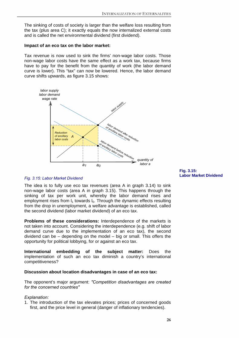
The sinking of costs of society is larger than the welfare loss resulting from the tax (plus area C); it exactly equals the now internalized external costs and is called the net environmental dividend (first dividend). Impact of an eco tax on the labor market: Tax revenue is now used to sink the firms’ non-wage labor costs. Those non-wage labor costs have the same effect as a work tax, because firms have to pay for the benefit from the quantity of work (the labor demand curve is lower). This “tax” can now be lowered. Hence, the labor demand curve shifts upwards, as figure 3.15 shows:

quantity of

labor aa1

labor supplylabor demand

wage rate

a0

A

labor supply

Reductionof ancillarylabor costs

labor demand after reduction

of ancillary labor costslabor demand before reduction

of ancillary labor costs

Fig. 3.15: Labor Market Dividend

The idea is to fully use eco tax revenues (area A in graph 3.14) to sink non-wage labor costs (area A in graph 3.15). This happens through the sinking of tax per work unit, whereby the labor demand rises and employment rises from l1 towards l0. Through the dynamic effects resulting from the drop in unemployment, a welfare advantage is established, called the second dividend (labor market dividend) of an eco tax. Problems of these considerations: Interdependence of the markets is not taken into account. Considering the interdependence (e.g. shift of labor demand curve due to the implementation of an eco tax), the second dividend can be – depending on the model – big or small. This offers the opportunity for political lobbying, for or against an eco tax. International embedding of the subject matter: Does the implementation of such an eco tax diminish a country’s international competitiveness? Discussion about location disadvantages in case of an eco tax: The opponent’s major argument: "Competition disadvantages are created for the concerned countries" Explanation: 1. The introduction of the tax elevates prices; prices of concerned goods

first, and the price level in general (danger of inflationary tendencies).

Fig. 3.15: Labor Market Dividend

CHAPTER 3

27

2. National revenue increases; hence, the national portion of the aggregate output rises.

3. Exportation opportunities decline due to an elevation in prices, which causes exportation loss.

4. The lift in prices of the concerned goods causes adjustment problems in the reorganization of the economy, including short to medium term employment problems.

Advocates respond: 1. In general, there are no significant price lifts of goods, since the

proportion of environmental costs of the total production costs are only 3 to 5 % on average. Only some branches, such as energy intensive production (high use of fossil energy) are concerned.

2. First Mover Advantage: The tax generates an incentive for implementing environmentally friendly technologies. If other countries introduce the eco tax later, the country can export its environmentally friendly technologies to those countries.

3. Structural change is attained by changing the structure of production from highly polluting to environmentally friendly goods. In other words, the structure of production becomes less energy intensive, and more labour intensive (this can lead to positive employment effects). However, temporary governmental subsidies might be required.

Conclusion: introducing an eco tax • The eco tax seems socially advantageous. • Due to lobbying activities or the political system and its corresponding

decision structures, difficulties in the realization can arise. In that case, the “secondary advantage” can be used as an additional argument: Idea:

- Secondary advantage occurs in the country itself - Secondary advantage occurs quickly - Secondary advantage is easily quantifyable

Examples of secondary advantage of a CO2 tax: - National pollution is reduced (measurable) - First Mover Advantage - Efficiency advantages thanks to structural change - Less dependency on non-renewable energy sources (and the

corresponding system, e.g. OPEC oil crisis). Bibliography Frey, René L.; Staehlin-Witt, Elke, Blöchiger, Hansjörg: Mit Ökonomie zur Ökologie, Basel/Frankfurt am Main, Stuttgart: Helbing&Lichtenhahn, 1993, 2nd edition, p. 55-65, 67-110, 173-177. Endres, Alfred: Umweltökonomie, Stuttgart/Berlin/Köln: Kohlhammer, 2000, p. 117-141, 208-245.

Documents

Chapter 3: INTERNALIZATION OF EXTERNALITIES