Lecture 5: Externalities (chapter 9)

• Relation to lectures 1-4

• Negative externalities

• Positive externalities: public goods and empathy

• Efficiency wage relation

• Nonconvexities

• Risk and uncertainty

Aim of lecture 5

• Show how positive and negative externalities can be included in general equilibrium models: public goods, empathy, pollution

• With specific emphasis on the effects of the introduction of an efficiency wage relation and social security arrangements

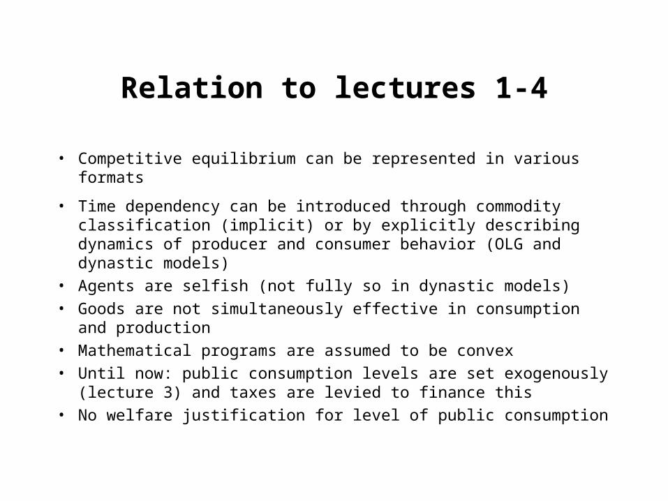
Relation to lectures 1-4

• Competitive equilibrium can be represented in various formats

• Time dependency can be introduced through commodity classification (implicit) or by explicitly describing dynamics of producer and consumer behavior (OLG and dynastic models)

• Agents are selfish (not fully so in dynastic models)

• Goods are not simultaneously effective in consumption and production

• Mathematical programs are assumed to be convex

• Until now: public consumption levels are set exogenously (lecture 3) and taxes are levied to finance this

• No welfare justification for level of public consumption

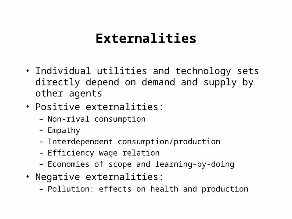
Externalities

• Individual utilities and technology sets directly depend on demand and supply by other agents

• Positive externalities:– Non-rival consumption

– Empathy

– Interdependent consumption/production

– Efficiency wage relation

– Economies of scope and learning-by-doing

• Negative externalities:– Pollution: effects on health and production

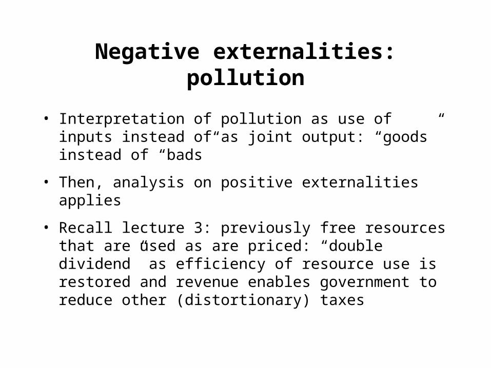
Negative externalities: pollution

• Interpretation of pollution as use of inputs instead of as joint output: “goods” instead of “bads”

• Then, analysis on positive externalities applies

• Recall lecture 3: previously free resources that are used as are priced: “double dividend” as efficiency of resource use is restored and revenue enables government to reduce other (distortionary) taxes

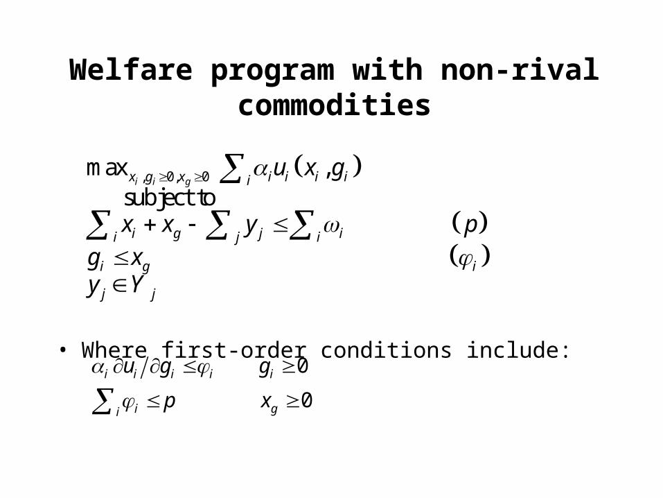
Welfare program with non-rival commodities

• Where first-order conditions include:

, 0, 0max , subject to

i i gx g x i i i ii

i g j ii j i

i g i

j j

u x g

x x y pg xy Y

0

0i i i i i

i gi

u g g

p x

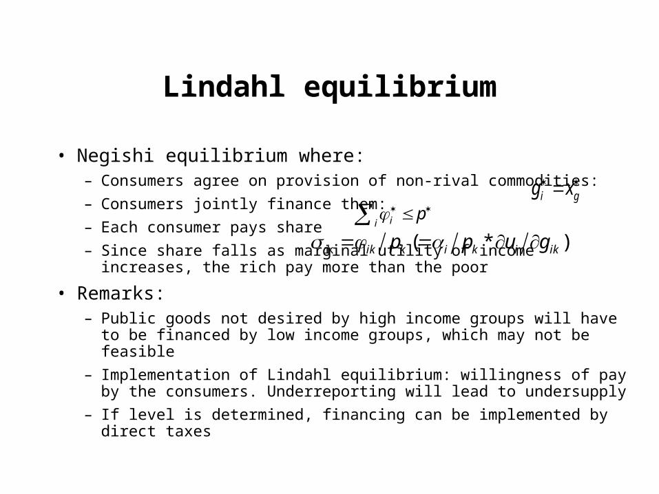
Lindahl equilibrium

• Negishi equilibrium where:– Consumers agree on provision of non-rival commodities:

– Consumers jointly finance them:

– Each consumer pays share

– Since share falls as marginal utility of income increases, the rich pay more than the poor

• Remarks:– Public goods not desired by high income groups will have to be

financed by low income groups, which may not be feasible

– Implementation of Lindahl equilibrium: willingness of pay by the consumers. Underreporting will lead to undersupply

– If level is determined, financing can be implemented by direct taxes

iip

i gg x

ik ( * )ik k i k i ikp p u g

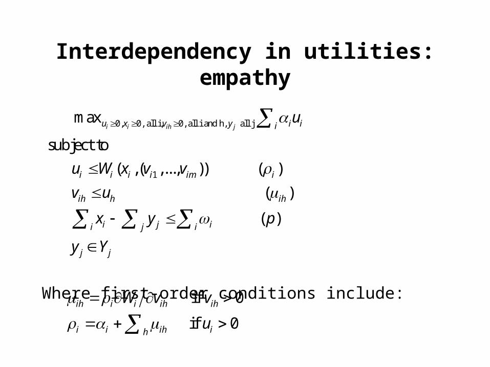
Interdependency in utilities: empathy

Where first-order conditions include:

0, 0, all i, 0, all i and h, all j

1

max

subject to

( ,( ,..., )) ( )

( )

i i ih ju x v y i ii

i i i i im i

ih h ih

i j ii j i

u

u W x v v

v u

x y

( )

j j

p

y Y

if 0

if 0ih i i ih ih

i i ih ih

W v v

u

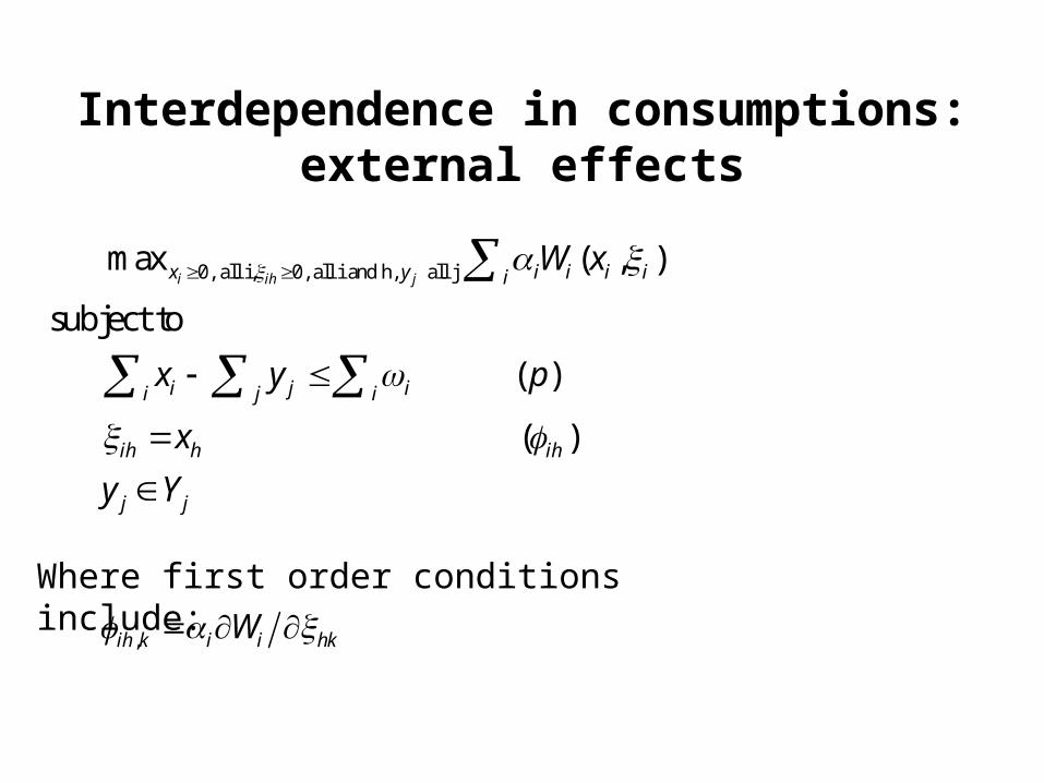
Interdependence in consumptions: external effects

0, all i, 0, all i and h, all j max ( , )

subject to

( )

( )

i ih jx y i i i ii

i j ii j i

ih h ih

j j

W x

x y p

x

y Y

Where first order conditions include:

,ih k i i hkW

Interdependency in utilities and consumptions

• Utility of other consumers cannot be observed; therefore, consumers imagine being the other person. Rawls’ “veil of ignorance”

• In a dynamic context, this other person could also represent the agent himself at an older age: savings result as transfers to this other person

• Note: consumption is a flow variable: consumers can also value the presence of stocks of commodities being available for (non-rival) consumption, such as nature parks. This requires representation of empathy within dynamic models of lecture 4

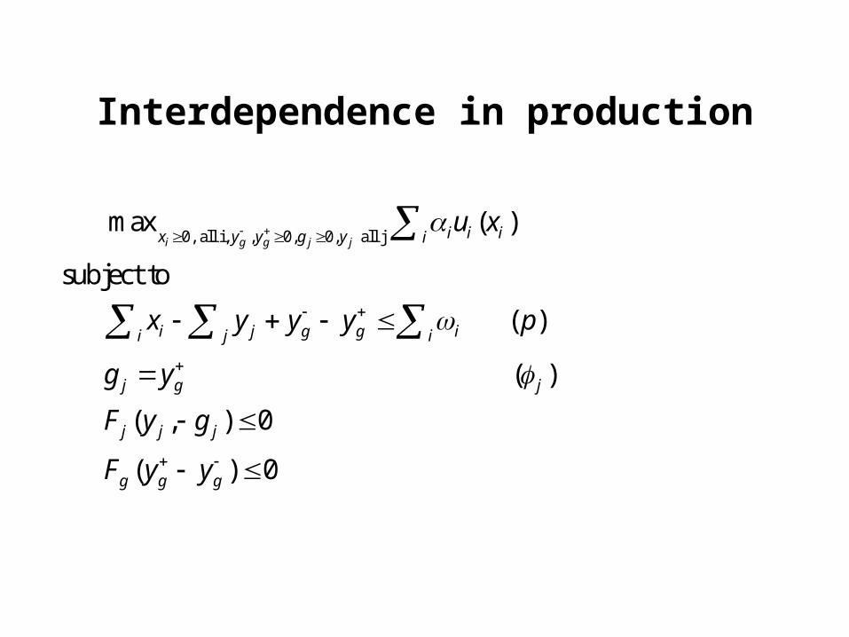
Interdependence in production

0, all i, , 0, 0, all j max ( )

subject to

( )

( )

( , ) 0

( )

i g g j ji i ix y y g y i

i j g g ii j i

j g j

j j j

g g g

u x

x y y y p

g y

F y g

F y y

0

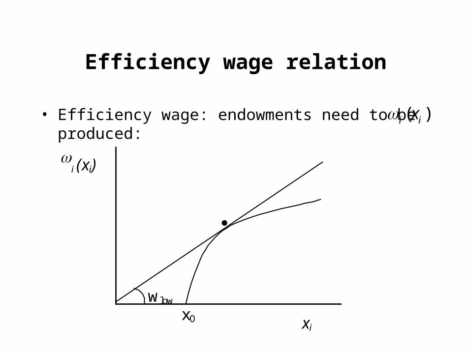
Efficiency wage relation

• Efficiency wage: endowments need to be produced:

i (xi)

xi

wlow

xO

( )i ix

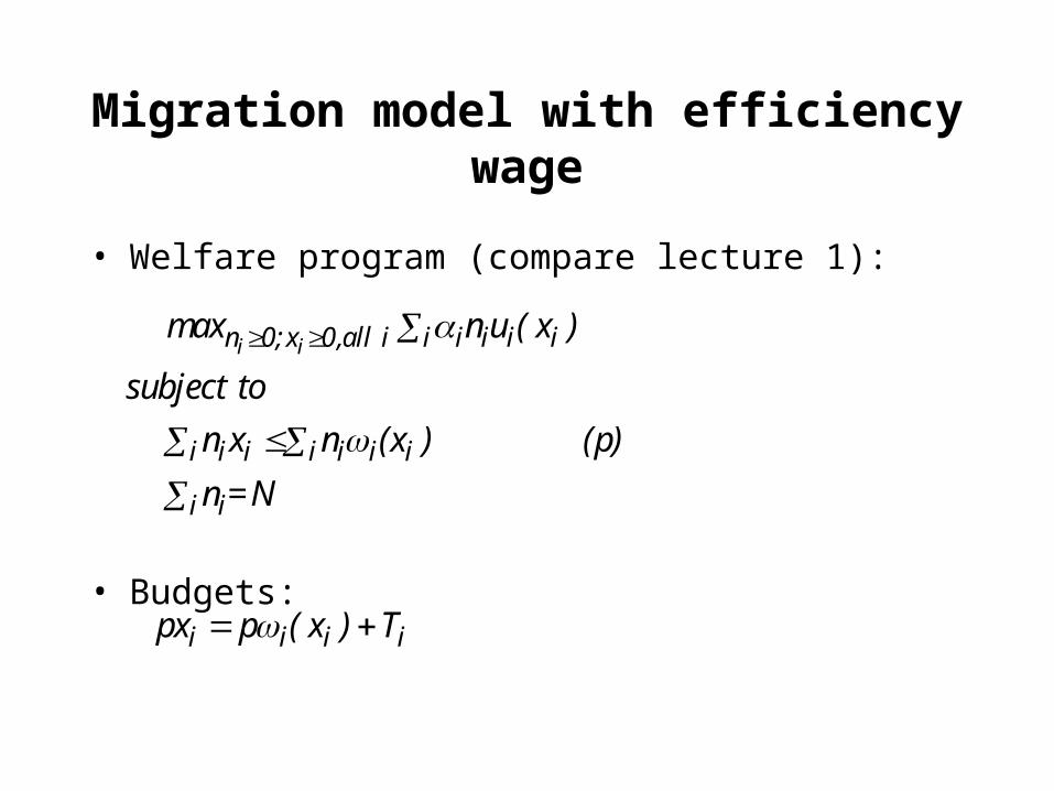
Migration model with efficiency wage

• Welfare program (compare lecture 1):

• Budgets:

i i in 0;x 0,all i i i i i

i ii i i i i

i i

max n u ( x )

subject to

n x n (x ) (p)

n =N

i i i ipx p ( x ) T

Efficiency wage

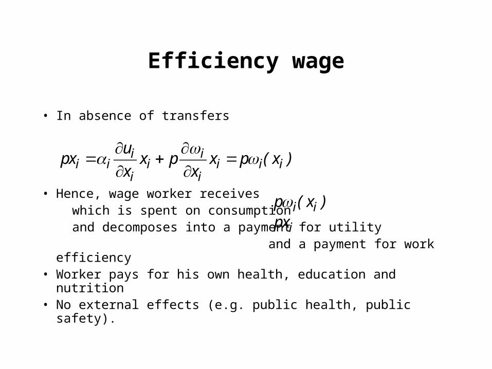
• In absence of transfers

• Hence, wage worker receives which is spent on consumption and decomposes into a payment for utility and a payment for work efficiency • Worker pays for his own health, education and nutrition• No external effects (e.g. public health, public safety).

i ii i i i i i

i i

upx x p x p ( x )

x x

i ip ( x )ipx

Efficiency wage and nonconvexities

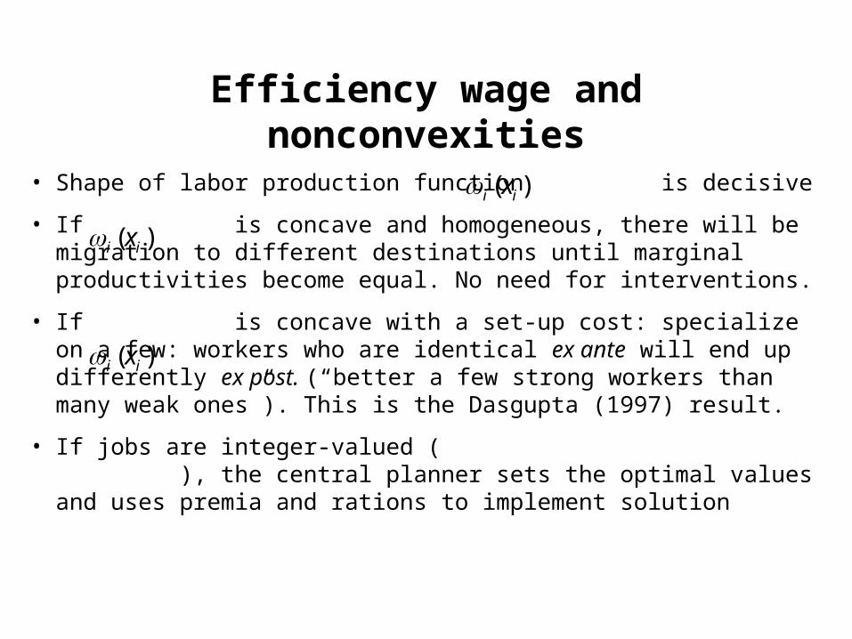
• Shape of labor production function is decisive

• If is concave and homogeneous, there will be migration to different destinations until marginal productivities become equal. No need for interventions.

• If is concave with a set-up cost: specialize on a few: workers who are identical ex ante will end up differently ex post. (“better a few strong workers than many weak ones”). This is the Dasgupta (1997) result.

• If jobs are integer-valued ( ), the central planner sets the optimal values and uses premia and rations to implement solution

( )i ix

( )i ix

( )i ix

Social security

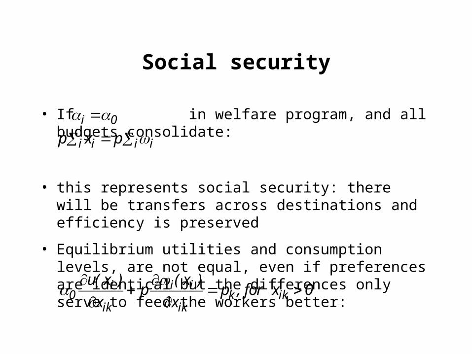
• If in welfare program, and all budgets consolidate:

• this represents social security: there will be transfers across destinations and efficiency is preserved

• Equilibrium utilities and consumption levels, are not equal, even if preferences are identical but the differences only serve to feed the workers better:

i 0

i ii ip x p

i i i0 k ik

ik ik

u( x ) ( x )p p , for x 0

x x

Efficiency wage and taxes

• Proportional tax on income:

• If endowments are given, no distortion

• However, in present formulation, consumer choice of consumption level is affected.

• In general, if consumption falls below critical level, productivity of consumers falls, and economy is trapped in underdevelopment equilibrium (Mirrlees, 1975).

(1 )( ( ) )i i i i ipx p x

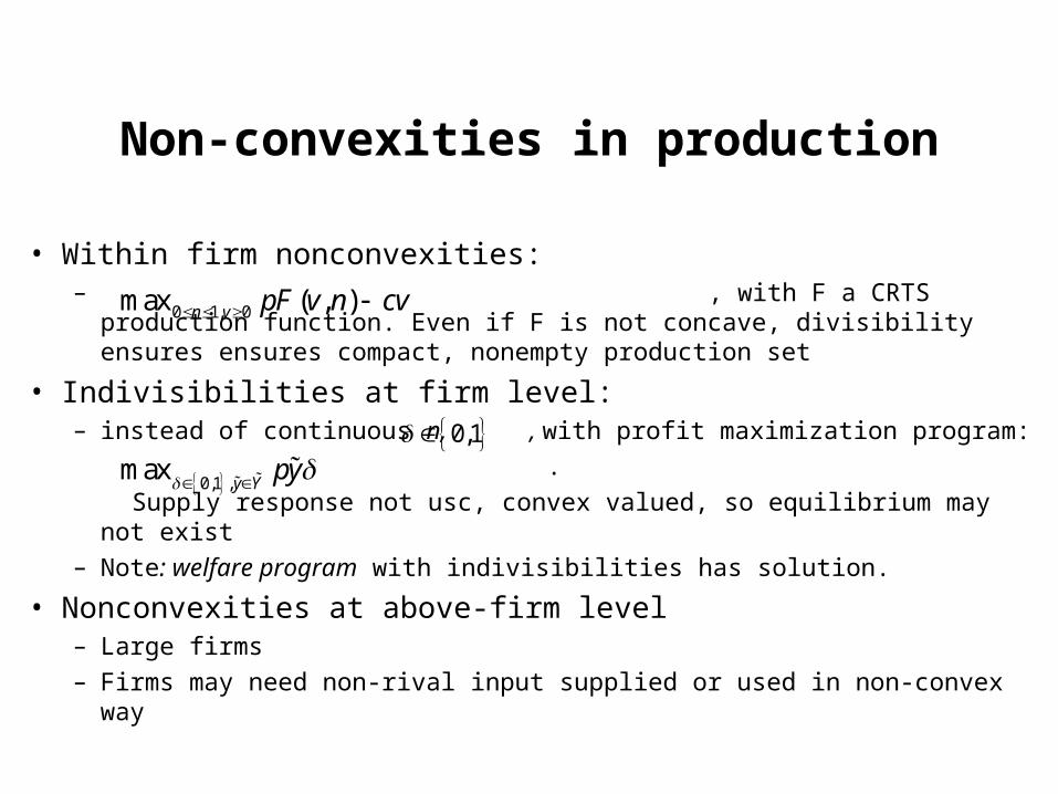
Non-convexities in production

• Within firm nonconvexities:– , with F a CRTS production function. Even if F is

not concave, divisibility ensures ensures compact, nonempty production set

• Indivisibilities at firm level: – instead of continuous n, , with profit maximization program:

.

Supply response not usc, convex valued, so equilibrium may not exist

– Note: welfare program with indivisibilities has solution.

• Nonconvexities at above-firm level– Large firms

– Firms may need non-rival input supplied or used in non-convex way

0 1, 0max ( , )n v pF v n cv

0,1

0,1 ,max

y Ypy

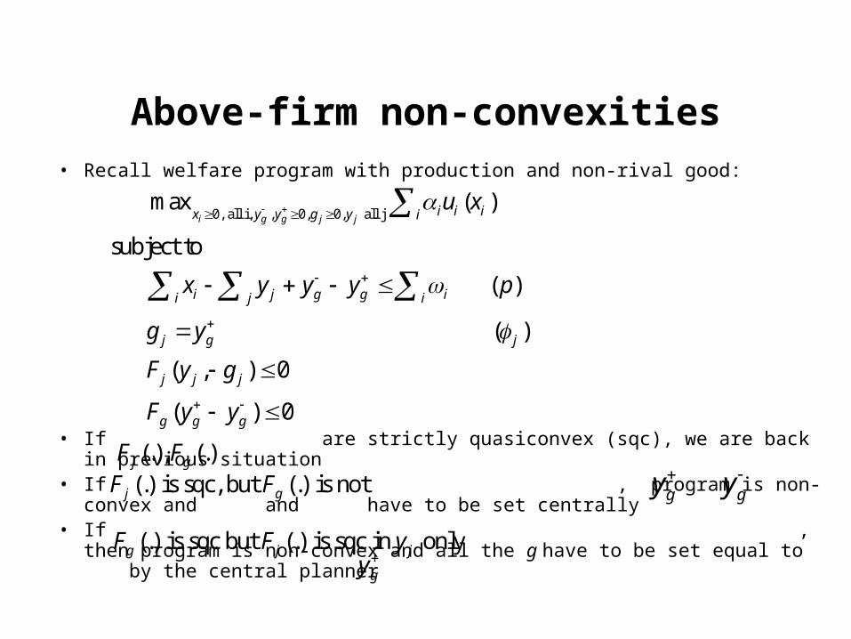
Above-firm non-convexities

• Recall welfare program with production and non-rival good:

• If are strictly quasiconvex (sqc), we are back in previous situation• If , program is non-convex and and have

to be set centrally• If , then program is non-convex and all

the g have to be set equal to by the central planner

0, all i, , 0, 0, all j max ( )

subject to

( )

( )

( , ) 0

( )

i g g j ji i ix y y g y i

i j g g ii j i

j g j

j j j

g g g

u x

x y y y p

g y

F y g

F y y

0

(.), (.)j gF F (.) is sqc, but (.) is notj gF F

(.) is sqc but (.) is sqc in onlyg j jF F y

gygy

gy

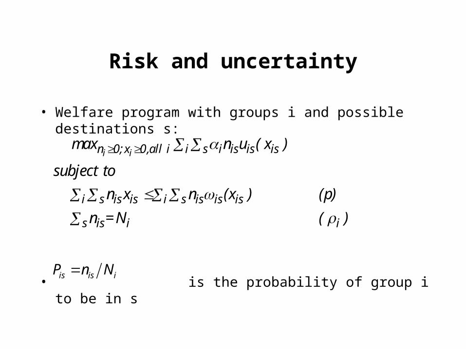
Risk and uncertainty

• Welfare program with groups i and possible destinations s:

• is the probability of group i to be in s

i i i sn 0;x 0,all i i is is is

i s i sis is is is is

s is i i

max n u ( x )

subject to

n x n (x ) (p)

n =N ( )

is is iP n N

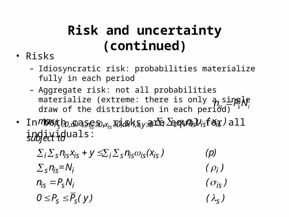
Risk and uncertainty (continued)• Risks

– Idiosyncratic risk: probabilities materialize fully in each period

– Aggregate risk: not all probabilities materialize (extreme: there is only a single draw of the distribution in each period)

• In both cases, risks are equal for all individuals: is s in P N

s is is i sP 0,all s,n 0,x 0,all i,s,y 0 i is is is

i s i sis is is is is

s is i i

is s

max n u ( x )

subject to

n x y n (x ) (p)

n =N ( )

n P

i is

s s s

N ( )

0 P P ( y ) ( )

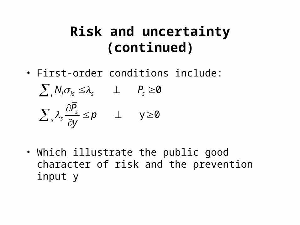
Risk and uncertainty (continued)

• First-order conditions include:

• Which illustrate the public good character of risk and the prevention input y

0

y 0

i is s si

sss

N P

Pp

y