Embed Size (px)
Citation preview
CHAPTER 3Image Segmentation Using Deformable Models
Chenyang XuThe Johns Hopkins University
Dzung L. PhamNational Institute of Aging
Jerry L. PrinceThe Johns Hopkins University
Contents
3.1 Introduction 131
3.2 Parametric deformable models 133
3.2.1 Energy minimizing formulation 134
3.2.2 Dynamic force formulation 136
3.2.3 External forces 138
3.2.4 Numerical implementation 144
3.2.5 Discussion 145
3.3 Geometric deformable models 146
3.3.1 Curve evolution theory 146
3.3.2 Level set method 147
3.3.3 Speed functions 150
3.3.4 Relationship to parametric deformable models 152
3.3.5 Numerical implementation 153
3.3.6 Discussion 154
3.4 Extensions of deformable models 154
3.4.1 Deformable Fourier models 155
3.4.2 Deformable models using modal analysis 157
3.4.3 Deformable superquadrics 159
3.4.4 Active shape models 161
3.4.5 Other models 167
3.5 Conclusion and future directions 167
129

130 Image Segmentation Using Deformable Models
3.6 Further reading 168
3.7 Acknowledgments 168
3.8 References 168

Introduction 131
3.1 Introduction
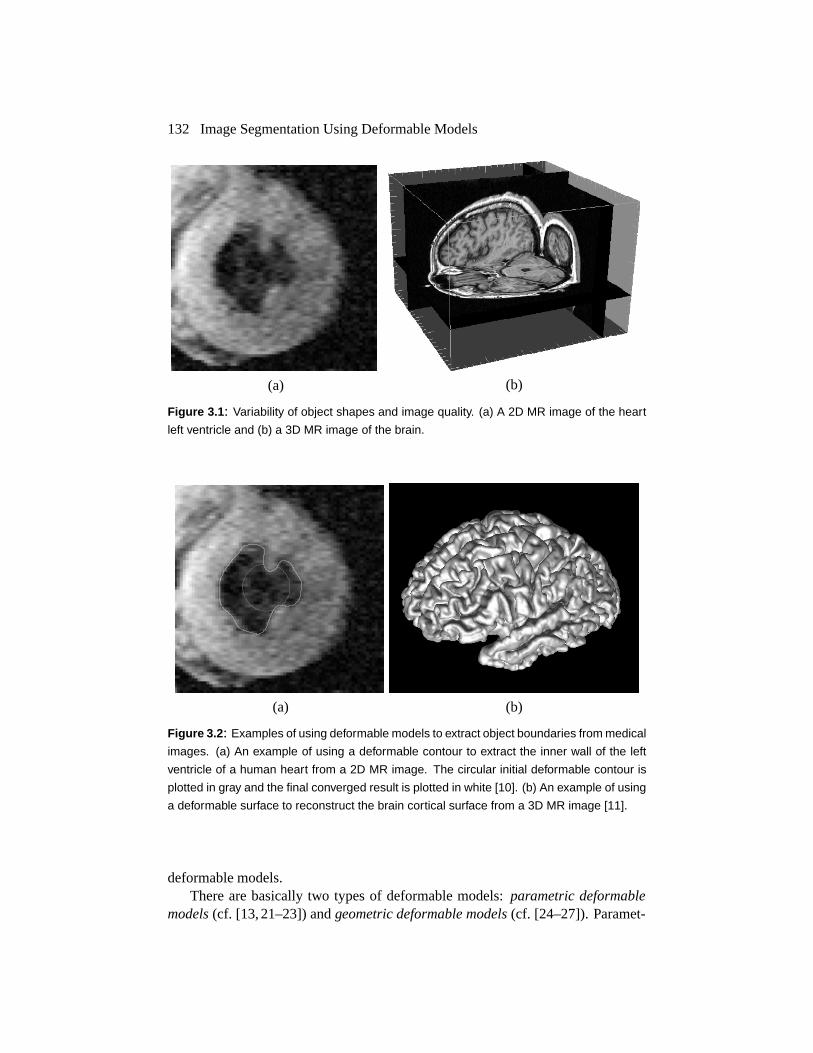
In the past four decades, computerized image segmentation has played an in-creasingly important role in medical imaging. Segmented images are now usedroutinely in a multitude of different applications, such as the quantification of tissuevolumes [1], diagnosis [2], localization of pathology [3], study of anatomical struc-ture [4, 5], treatment planning [6], partial volume correction of functional imagingdata [7], and computer-integrated surgery [8, 9]. Image segmentation remains adifficult task, however, due to both the tremendous variability of object shapes andthe variation in image quality (see Fig. 3.1). In particular, medical images are oftencorrupted by noise and sampling artifacts, which can cause considerable difficul-ties when applying classical segmentation techniques such as edge detection andthresholding. As a result, these techniques either fail completely or require somekind of postprocessing step to remove invalid object boundaries in the segmentationresults.
To address these difficulties, deformable models have been extensively stud-ied and widely used in medical image segmentation, with promising results. De-formable models are curves or surfaces defined within an image domain that canmove under the influence of internal forces, which are defined within the curve orsurface itself, and external forces, which are computed from the image data. Theinternal forces are designed to keep the model smooth during deformation. The ex-ternal forces are defined to move the model toward an object boundary or other de-sired features within an image. By constraining extracted boundaries to be smoothand incorporating other prior information about the object shape, deformable mod-els offer robustness to both image noise and boundary gaps and allow integratingboundary elements into a coherent and consistent mathematical description. Sucha boundary description can then be readily used by subsequent applications. More-over, since deformable models are implemented on the continuum, the resultingboundary representation can achieve subpixel accuracy, a highly desirable prop-erty for medical imaging applications. Figure 3.2 shows two examples of usingdeformable models to extract object boundaries from medical images. The result isa parametric curve in Fig. 3.2(a) and a parametric surface in Fig. 3.2(b).
Although the term deformable models first appeared in the work by Terzopou-los and his collaborators in the late eighties [12–15], the idea of deforming a tem-plate for extracting image features dates back much farther, to the work of Fis-chler and Elschlager’s spring-loaded templates [16] and Widrow’s rubber masktechnique [17]. Similar ideas have also been used in the work by Blake and Zis-serman [18], Grenander et al. [19], and Miller et al. [20]. The popularity of de-formable models is largely due to the seminal paper “Snakes: Active Contours” byKass, Witkin, and Terzopoulos [13]. Since its publication, deformable models havegrown to be one of the most active and successful research areas in image seg-mentation. Various names, such as snakes, active contours or surfaces, balloons,and deformable contours or surfaces, have been used in the literature to refer to
132 Image Segmentation Using Deformable Models
(a) (b)
Figure 3.1: Variability of object shapes and image quality. (a) A 2D MR image of the heart
left ventricle and (b) a 3D MR image of the brain.
(a) (b)
Figure 3.2: Examples of using deformable models to extract object boundaries from medical
images. (a) An example of using a deformable contour to extract the inner wall of the left
ventricle of a human heart from a 2D MR image. The circular initial deformable contour is
plotted in gray and the final converged result is plotted in white [10]. (b) An example of using
a deformable surface to reconstruct the brain cortical surface from a 3D MR image [11].
deformable models.There are basically two types of deformable models: parametric deformable
models (cf. [13, 21–23]) and geometric deformable models (cf. [24–27]). Paramet-

Parametric deformable models 133
ric deformable models represent curves and surfaces explicitly in their paramet-ric forms during deformation. This representation allows direct interaction withthe model and can lead to a compact representation for fast real-time implemen-tation. Adaptation of the model topology, however, such as splitting or mergingparts during the deformation, can be difficult using parametric models. Geomet-ric deformable models, on the other hand, can handle topological changes natu-rally. These models, based on the theory of curve evolution [28–31] and the levelset method [32, 33], represent curves and surfaces implicitly as a level set of ahigher-dimensional scalar function. Their parameterizations are computed onlyafter complete deformation, thereby allowing topological adaptivity to be easilyaccommodated. Despite this fundamental difference, the underlying principles ofboth methods are very similar.
This chapter is organized as follows. We first introduce parametric deformablemodels in Section 3.2, and then describe geometric deformable models in Sec-tion 3.3. An explicit mathematical relationship between parametric deformablemodels and geometric deformable models is presented in Section 3.3.4. In Sec-tion 3.4, we provide an overview of several extensions to these deformable models.Finally, in Section 3.5, we conclude the chapter and point out future research di-rections. We focus on describing the fundamentals of deformable models and theirapplication to image segmentation. Treatment of related work using deformablemodels in other applications such as image registration and motion estimation isbeyond the scope of this chapter. We refer readers interested in these other appli-cations to Section 3.6, where suggestions for further reading are given.
We note that although this chapter primarily deals with 2D deformable models(i.e., deformable contours), the principles discussed here apply to 3D deformablemodels (i.e., deformable surfaces) as well (cf. [23, 34]).
3.2 Parametric deformable models
In this section, we first describe two different types of formulations for para-metric deformable models: an energy minimizing formulation and a dynamic forceformulation. Although these two formulations lead to similar results, the first for-mulation has the advantage that its solution satisfies a minimum principle whereasthe second formulation has the flexibility of allowing the use of more general typesof external forces. We then present several commonly used external forces that caneffectively attract deformable models toward the desired image features. A numer-ical implementation of 2D deformable models or deformable contours is describedat the end of this section. Since the implementation of 3D deformable models ordeformable surfaces is more sophisticated than those of deformable contours, weprovide several references in Section 3.2.4 for additional reading rather than pre-senting an actual implementation.

134 Image Segmentation Using Deformable Models
Figure 3.3: A potential energy function derived from Fig. 3.1(a).
3.2.1 Energy minimizing formulation
The basic premise of the energy minimizing formulation of deformable con-tours is to find a parameterized curve that minimizes the weighted sum of inter-nal energy and potential energy. The internal energy specifies the tension or thesmoothness of the contour. The potential energy is defined over the image domainand typically possesses local minima at the image intensity edges occurring at ob-ject boundaries (see Fig. 3.3). Minimizing the total energy yields internal forcesand potential forces. Internal forces hold the curve together (elasticity forces)and keep it from bending too much (bending forces). External forces attract thecurve toward the desired object boundaries. To find the object boundary, paramet-ric curves are initialized within the image domain, and are forced to move towardthe potential energy minima under the influence of both these forces.
Mathematically, a deformable contour is a curve ���� � ������ � ����, � ���� ��, which moves through the spatial domain of an image to minimize the follow-ing energy functional:
���� � ���� � ���� � (3.1)
The first term is the internal energy functional and is defined to be
���� ��
�
� �
�
����
�������������
� ����
���������������
�� � (3.2)
The first-order derivative discourages stretching and makes the model behave likean elastic string. The second-order derivative discourages bending and makes the

Parametric deformable models 135
model behave like a rigid rod. The weighting parameters ���� and ���� can be usedto control the strength of the model’s tension and rigidity, respectively. In practice,���� and ���� are often chosen to be constants.
The second term is the potential energy functional and is computed by integrat-ing a potential energy function �� �� along the contour����:
���� �
� �
�
�������� � (3.3)
The potential energy function �� �� is derived from the image data and takessmaller values at object boundaries as well as other features of interest. Givena gray-level image ��� �� viewed as a function of continuous position variables�� ��, a typical potential energy function designed to lead a deformable contourtoward step edges is
�� �� � � � ������� �� � ��� ����� � (3.4)
where � is a positive weighting parameter, ���� �� is a two-dimensional Gaus-sian function with standard deviation �, � is the gradient operator, and � is the2D image convolution operator. If the desired image features are lines, then theappropriate potential energy function can be defined as follows:
�� �� � ������ �� � ��� ��� � (3.5)
where � is a weighting parameter. Positive � is used to find black lines on a whitebackground, while negative � is used to find white lines on a black background.For both edge and line potential energies, increasing � can broaden its attractionrange. However, larger � can also cause a shift in the boundary location, resultingin a less accurate result (this problem can be addressed by using potential energiescalculated with different values of �; see Section 3.2.3).
Regardless of the selection of the exact potential energy function, the proce-dure for minimizing the energy functional is the same. The problem of findinga curve ���� that minimizes the energy functional � is known as a variationalproblem [35]. It has been shown that the curve that minimizes � must satisfy thefollowing Euler-Lagrange equation [13, 22]:
�
��
����
��
��
��
���
�����
���
��� ��� � � � (3.6)
To gain some insight about the physical behavior of deformable contours, we canview Eq. (3.6) as a force balance equation
� ������ � � ������ � � � (3.7)
136 Image Segmentation Using Deformable Models
where the internal force is given by
� ������ ��
��
����
��
��
��
���
�����
���
�(3.8)
and the potential force is given by
� ������ � �� ��� � (3.9)
The internal force� ��� discourages stretching and bending while the potential force� ��� pulls the contour toward the desired object boundaries. In this chapter, wedefine the forces, derived from the potential energy function �� �� given in eitherEq. (3.4) or Eq. (3.5), as Gaussian potential forces.
To find a solution to Eq. (3.6), the deformable contour is made dynamic bytreating ���� as a function of time � as well as � — i.e., ���� ��. The partialderivative of � with respect to � is then set equal to the left-hand side of Eq. (3.6)as follows:
���
���
�
��
����
��
��
��
���
�����
���
��� ��� � (3.10)
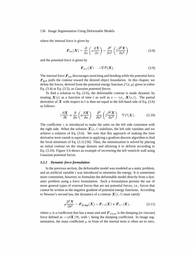
The coefficient � is introduced to make the units on the left side consistent withthe right side. When the solution ���� �� stabilizes, the left side vanishes and weachieve a solution of Eq. (3.6). We note that this approach of making the timederivative term vanish is equivalent to applying a gradient descent algorithm to findthe local minimum of Eq. (3.1) [34]. Thus, the minimization is solved by placingan initial contour on the image domain and allowing it to deform according toEq. (3.10). Figure 3.4 shows an example of recovering the left ventricle wall usingGaussian potential forces.
3.2.2 Dynamic force formulation
In the previous section, the deformable model was modeled as a static problem,and an artificial variable � was introduced to minimize the energy. It is sometimesmore convenient, however, to formulate the deformable model directly from a dyn-amic problem using a force formulation. Such a formulation permits the use ofmore general types of external forces that are not potential forces, i.e., forces thatcannot be written as the negative gradient of potential energy functions. Accordingto Newton’s second law, the dynamics of a contour���� �� must satisfy
����
���� � ����� � � ������ � � ������ � (3.11)
where � is a coefficient that has a mass unit and � �� is the damping (or viscous)force defined as �������, with � being the damping coefficient. In image seg-mentation, the mass coefficient � in front of the inertial term is often set to zero,
Parametric deformable models 137
(a)
(b)
Figure 3.4: An example of recovering the left ventricle wall using Gaussian potential forces.
(a) Gaussian potential forces and (b) the result of applying Gaussian potential forces to a
deformable contour, with the circular initial contour shown in gray and the final deformed
contour in white.

138 Image Segmentation Using Deformable Models
since the inertial term may cause the contour to pass over the weak edges. Thedynamics of the deformable contour without the inertial term becomes
���
��� � ������ � � ������ � (3.12)
The internal forces are the same as specified in Eq. (3.8). The external forces canbe either potential forces or nonpotential forces. We note, however, nonpotentialforces cannot be derived from the variational energy formulation of the previoussection. An alternate variational principle does exist (see [36]); however, it is notphysically intuitive.
External forces are often expressed as the superposition of several differentforces:
� ������ � � ���� � � ���� � � � �� �� ��� �
where � is the total number of external forces. This superposition formulationallows the external forces to be broken down into more manageable terms. Forexample, one might define the external forces to be composed of both Gaussianpotential forces and pressure forces, which are described in the next section.
3.2.3 External forces
In this section, we describe several kinds of external forces for deformablemodels. These external forces are applicable to both deformable contours and de-formable surfaces.
Multiscale Gaussian potential forceWhen using the Gaussian potential force described in Section 3.2.1, � must
be selected to have a small value in order for the deformable model to follow theboundary accurately. As a result, the Gaussian potential force can only attract themodel toward the boundary when it is initialized nearby. To remedy this problem,Terzopoulos, Witkin, and Kass [13, 15] proposed using Gaussian potential forcesat different scales to broaden its attraction range while maintaining the model’sboundary localization accuracy. The basic idea is to first use a large value of � tocreate a potential energy function with a broad valley around the boundary. Thecoarse-scale Gaussian potential force attracts the deformable contour or surfacetoward the desired boundaries from a long range. When the contour or surfacereaches equilibrium, the value of � is then reduced to allow tracking of the bound-ary at a finer scale. This scheme effectively extends the attraction range of theGaussian potential force. A weakness of this approach, however, is that there isno established theorem for how to schedule changes in �. The ad hoc schedulingschemes that are available may therefore lead to unreliable results.
Pressure forceCohen [22] proposed to increase the attraction range by using a pressure force
together with the Gaussian potential force. The pressure force can either inflate or

Parametric deformable models 139
deflate the model; hence, it removes the requirement to initialize the model nearthe desired object boundaries. Deformable models that use pressure forces are alsoknown as balloons [22].
The pressure force is defined as
� ���� � ����� � (3.13)
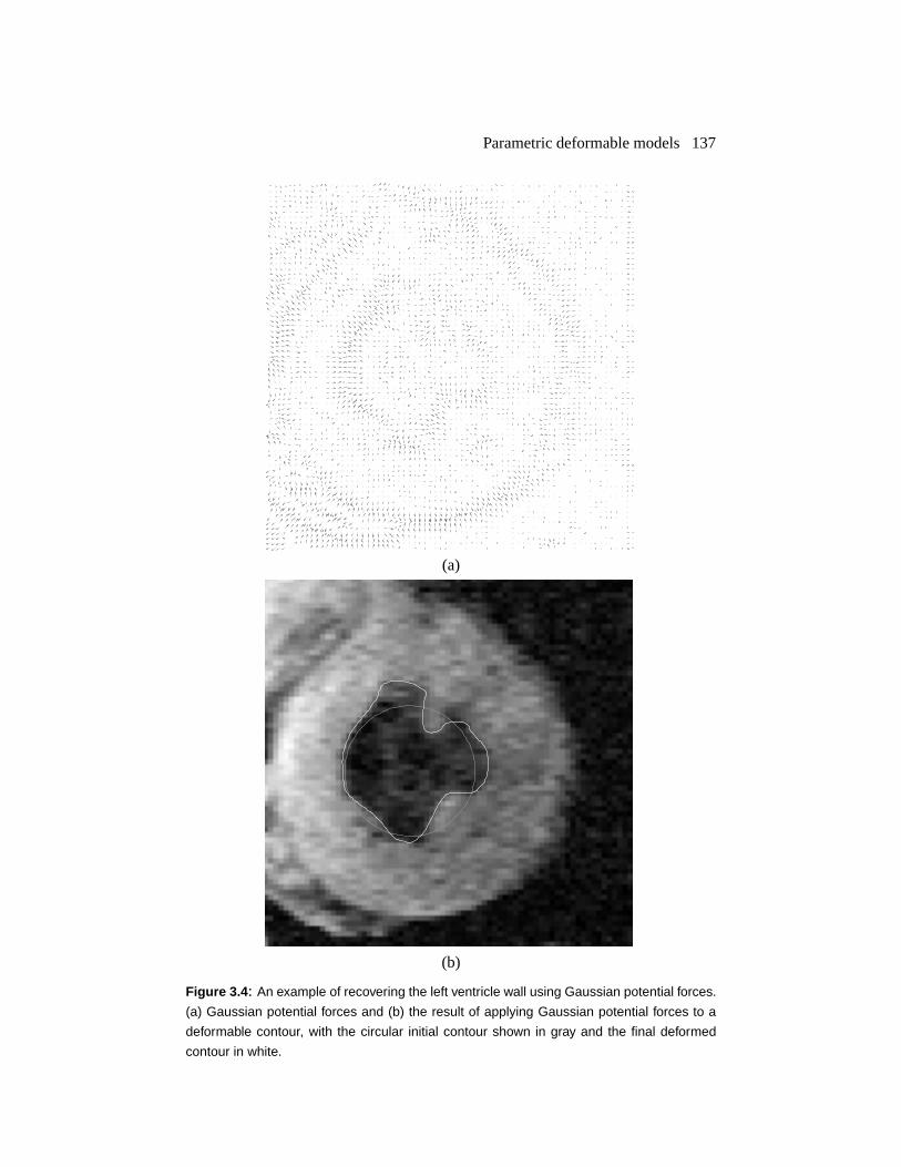
where ���� is the inward unit normal1 of the model at the point � and � is aconstant weighting parameter. The sign of � determines whether to inflate or de-flate the model and is typically chosen by the user. Recently, region information hasbeen used to define � with a spatial-varying sign based upon whether the modelis inside or outside the desired object (see [37, 38]). The value of � determinesthe strength of the pressure force. It must be carefully selected so that the pressureforce is slightly smaller than the Gaussian potential force at significant edges, butlarge enough to pass through weak or spurious edges. When the model deforms,the pressure force keeps inflating or deflating the model until it is stopped by theGaussian potential force. An example of using deformable contour with an inflat-ing pressure force is shown in Fig. 3.5. A disadvantage in using pressure forces isthat they may cause the deformable model to cross itself and form loops (cf. [39]).
Distance potential forceAnother approach for extending attraction range is to define the potential energy
function using a distance map as proposed by Cohen and Cohen [40]. The valueof the distance map at each pixel is obtained by calculating the distance betweenthe pixel and the closest boundary point, based either on Euclidean distance [41]or Chamfer distance [42]. By defining the potential energy function based on thedistance map, one can obtain a potential force field that has a large attraction range.
Given a computed distance map ��� ��, one way of defining a correspondingpotential energy, introduced in [40], is as follows:
��� �� � � � ������ ���� � (3.14)
The corresponding potential force field is given by ����� ��.
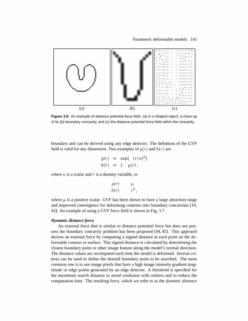
Gradient vector flowThe distance potential force is based on the principle that the model point
should be attracted to the nearest edge points. This principle, however, can causedifficulties when deforming a contour or surface into boundary concavities [43].A 2D example is shown in Fig. 3.6, where a U-shaped object and a close-up ofits distance potential force field within the boundary concavity is depicted. Notice
1In the parametric formulation of deformable models, the normal direction is sometimes assumedto be outward. Here we assume an inward direction for consistency with the geometric formulationof deformable models introduced in Section 3.3.
140 Image Segmentation Using Deformable Models
(a) (b) (c)
(d) (e) (f)
Figure 3.5: An example of pressure forces driven deformable contours. (a) Intensity CT
image slice of the left ventricle. (b) Edge detected image. (c) Initial deformable contour. (d)-
(f) Deformable contour moving toward the left ventricle boundary, driven by inflating pressure
force. Images courtesy of McInerney and Terzopoulos [23], The University of Toronto.
that at the concavity, distance potential forces point horizontally in opposite direc-tions, thus preventing the contour from converging into the boundary concavity. Toaddress this problem, Xu and Prince [10, 43] employed a vector diffusion equa-tion that diffuses the gradient of an edge map in regions distant from the boundary,yielding a different force field called the gradient vector flow (GVF) field. Theamount of diffusion adapts according to the strength of edges to avoid distortingobject boundaries.
A GVF field is defined as the equilibrium solution to the following vector partialdifferential equation:
��
��� ����� ����� � ����� ���� ���� � (3.15)
where ��� �� �� � �� , ����� denotes the partial derivative of ��� �� �� withrespect to �, �� is the Laplacian operator (applied to each spatial component of� separately), and � is an edge map that has higher value at the desired object
Parametric deformable models 141
(a) (b) (c)
Figure 3.6: An example of distance potential force field. (a) A U-shaped object, a close-up
of its (b) boundary concavity, and (c) the distance potential force field within the concavity.
boundary and can be derived using any edge detector. The definition of the GVFfield is valid for any dimension. Two examples of ���� and ���� are
���� � ��������
���� � �� ���� �
where � is a scalar and � is a dummy variable, or
���� � �
���� � �� �
where � is a positive scalar. GVF has been shown to have a large attraction rangeand improved convergence for deforming contours into boundary concavities [10,43]. An example of using a GVF force field is shown in Fig. 3.7.
Dynamic distance forceAn external force that is similar to distance potential force but does not pos-
sess the boundary concavity problem has been proposed [44, 45]. This approachderives an external force by computing a signed distance at each point on the de-formable contour or surface. This signed distance is calculated by determining theclosest boundary point or other image feature along the model’s normal direction.The distance values are recomputed each time the model is deformed. Several cri-teria can be used to define the desired boundary point to be searched. The mostcommon one is to use image pixels that have a high image intensity gradient mag-nitude or edge points generated by an edge detector. A threshold is specified forthe maximum search distance to avoid confusion with outliers and to reduce thecomputation time. The resulting force, which we refer to as the dynamic distance

142 Image Segmentation Using Deformable Models
(a)
(b)
Figure 3.7: An example of the gradient vector flow driven deformable contours. (a) A
gradient vector flow force field and (b) the result of applying gradient vector flow force to a
deformable contour, with the circular initial contour shown in gray and the final deformed
contour in white.
Parametric deformable models 143
force, can attract deformable models to the desired image feature from a fairly longrange limited only by the threshold.
Given a point � on the contour or surface, its inward unit normal ����,the computed signed distance ����, and a specified distance threshold ��, atypical definition for the dynamic distance force is
����� � �����
��
���� � (3.16)
The weakness of this method is that a relatively time-consuming 1D searchalong the normal direction must be performed each time the model deforms. Settingthe search distance threshold lower can reduce the run time but has the undesirableside effect of decreasing the attraction range of the dynamic distance force.
Interactive forceIn many clinical situations, it is important to allow an operator to interact with
the deformable model as it is deforming. This interaction improves the accuracy ofthe segmentation result when automated external forces fail to deform the modelto the desired feature in certain regions. For example, the user may want to pullthe model toward significant image features, or would like to constrain the modelso that it must pass through a set of landmark points identified by an expert. De-formable models allow these kinds of user interactions to be conveniently modeledas additional force terms.
Two kinds of commonly used interactive forces are spring forces and volcanoforces, proposed by Kass et al. [13]. Spring forces are defined to be proportional tothe distance between a point � on the model and a user-specified point �:
� � � ������ � (3.17)
Spring forces act to pull the model toward �. The further away the model is from�, the stronger the pulling force. The point � is selected by finding the closestpoint on the model to � using a heuristic search around a local neighborhood of �.An example of using spring forces is shown in Fig. 3.8.
Volcano forces are designed to push the model away from a local region arounda “volcano” point �. For computational efficiency, the force is only computed in aneighborhood � ��� as follows:
� ���� �
� �
����� � � � ���
� � �� � ���� (3.18)
where � � � � �. Note that the magnitude of the forces is limited near � � � toavoid numerical instability. Another possible definition for volcano forces is
� ���� �
� � ���
�������
� ���� � � � ���
� � �� � ���� (3.19)
where �� is used to adjust the strength distribution of the volcano force.

144 Image Segmentation Using Deformable Models
(a) (b)
Figure 3.8: Example of interactive forces. (a) A CT image slice of a canine left ventricle. (b)
A deformable contour moves toward high gradients in the edge detected image, influenced
by landmark points near the center of the image and a spring force that pulls the contour
toward an edge at the bottom right. Image courtesy of McInerney and Terzopoulos [23], The
University of Toronto.
3.2.4 Numerical implementation
Various numerical implementations of deformable models have been reportedin the literature. For examples, the finite difference method [13], dynamic program-ming [21], and greedy algorithm [46] have been used to implement deformable con-tours, while finite difference methods [15] and finite element methods [23, 34, 47]have been used to implement deformable surfaces. The finite difference method re-quires only local operations and is efficient to compute. The finite element method,on the other hand, is more costly to compute but has the advantage of being welladapted to the irregular mesh representations of deformable surfaces. In this sec-tion, we present the finite difference method implementation for deformable con-tours as described in [13].
Since the numerical scheme proposed by [13] does not require external forcesto be potential forces, it can be used to implement deformable contours using ei-ther potential forces or nonpotential forces. By approximating the derivatives inEq. (3.12) with finite differences, and converting to the vector notation
Parametric deformable models 145
� � ��
� � � � ������ ����� � ���� �����, we can rewrite Eq. (3.12) as
��
����
���
�
���� ���
� ��
�� ���
��
����
��
��������
�� � ��
�� �� �
������� � ��
�� ��
�� ��� � ��
� �� ��� � � �����
�� �(3.20)
where � is the damping coefficient, � � �����, � � �����, � the step size inspace, and �� the step size in time. In general, the external force � ��� is stored as adiscrete vector field, i.e., a finite set of vectors defined on an image grid. The valueof � ��� at any location � can be obtained through a bilinear interpolation of theexternal force values at the grid points near � .
Equation (3.20) can be written in a compact matrix form as
� ����
�� �� � � �����
��� � (3.21)
where � � ����, �, ���, and � �������� are � � � matrices, and � is an
� �� pentadiagonal banded matrix with � being the number of sample points.Equation (3.21) can then be solved iteratively by matrix inversion using the follow-ing equation:
� � �� � ��������� � �� ��������� � (3.22)
The inverse of the matrix � � �� can be calculated efficiently by LU decom-position2. The decomposition needs only to be performed once for deformationprocesses that do not alter the elasticity or rigidity parameters.
3.2.5 Discussion
So far, we have formulated the deformable model as a continuous curve orsurface. In practice, however, it is sometimes more straightforward to design thedeformable models from a discrete point of view. Example of work in this areaincludes [48–53].
Parametric deformable models have been applied successfully in a wide rangeof applications; however, they have two main limitations. First, in situations wherethe initial model and the desired object boundary differ greatly in size and shape,the model must be reparameterized dynamically to faithfully recover the objectboundary. Methods for reparameterization in 2D are usually straightforward andrequire moderate computational overhead. Reparameterization in 3D, however, re-quires complicated and computationally expensive methods. The second limitation
2LU decomposition stands for Lower and Upper triangular decomposition, a well-known tech-nique in linear algebra.
146 Image Segmentation Using Deformable Models
with the parametric approach is that it has difficulty dealing with topological adap-tation such as splitting or merging model parts, a useful property for recovering ei-ther multiple objects or an object with unknown topology. This difficulty is causedby the fact that a new parameterization must be constructed whenever the topologychange occurs, which requires sophisticated schemes [54, 55].
3.3 Geometric deformable models
Geometric deformable models, proposed independently by Caselles et al. [24]and Malladi et al. [25], provide an elegant solution to address the primary limita-tions of parametric deformable models. These models are based on curve evolutiontheory [28–31] and the level set method [32, 33]. In particular, curves and sur-faces are evolved using only geometric measures, resulting in an evolution thatis independent of the parameterization. As in parametric deformable models, theevolution is coupled with the image data to recover object boundaries. Since theevolution is independent of the parameterization, the evolving curves and surfacescan be represented implicitly as a level set of a higher-dimensional function. As aresult, topology changes can be handled automatically.
In this section, we first review the fundamental concepts in curve evolution the-ory and the level set method. We next present three types of geometric deformablemodels, the difference being in the design of speed functions. We then show amathematical relationship between a particular class of parametric and geometricmodels. Next, we describe a numerical implementation of geometric deformablemodels proposed by Osher and Sethian [32] in Section 3.3.5. Finally, at the end ofthis section we compare geometric deformable models with parametric deformablemodels. We note that although the geometric deformable models are presentedin 2D, their formulation can be directly extended to 3D. A thorough treatment onevolving curves and surfaces using the level set representation can be found in [33].
3.3.1 Curve evolution theory
The purpose of curve evolution theory is to study the deformation of curvesusing only geometric measures such as the unit normal and curvature as opposedto the quantities that depend on parameters such as the derivatives of an arbitraryparameterized curve. Let us consider a moving curve ���� �� � ����� ��� � ��� ���,where � is any parameterization and � is the time, and denote its inward unit normalas � and its curvature as �, respectively. The evolution of the curve along itsnormal direction can be characterized by the following partial differential equation:
��
��� � ���� � (3.23)
where � ��� is called speed function, since it determines the speed of the curveevolution. We note that a curve moving in some arbitrary direction can always bereparameterized to have the same form as Eq. (3.23) [56]. The intuition behind this
Geometric deformable models 147
fact is that the tangent deformation affects only the curve’s parameterization, notits shape and geometry.
The most extensively studied curve deformations in curve evolution theory arecurvature deformation and constant deformation. Curvature deformation is givenby the so-called geometric heat equation
��
��� ��� �
where � is a positive constant. This equation will smooth a curve, eventuallyshrinking it to a circular point [57]. The use of the curvature deformation hasan effect similar to the use of the elastic internal force in parametric deformablemodels.
Constant deformation is given by
��
��� ��� �
where �� is a coefficient determining the speed and direction of deformation. Con-stant deformation plays the same role as the pressure force in parametric deformablemodels. The properties of curvature deformation and constant deformation arecomplementary to each other. Curvature deformation removes singularities bysmoothing the curve, while constant deformation can create singularities from aninitially smooth curve.
The basic idea of the geometric deformable model is to couple the speed ofdeformation (using curvature and/or constant deformation) with the image data, sothat the evolution of the curve stops at object boundaries. The evolution is im-plemented using the level set method. Thus, most of the research in geometricdeformable models has been focused in the design of speed functions. We reviewseveral representative speed functions in Section 3.3.3.
3.3.2 Level set method
We now review the level set method for implementing curve evolution. Thelevel set method is used to account for automatic topology adaptation, and it alsoprovides the basis for a numerical scheme that is used by geometric deformablemodels. The level set method for evolving curves is due to Osher and Sethian [32,58, 59].
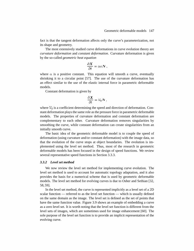
In the level set method, the curve is represented implicitly as a level set of a 2Dscalar function — referred to as the level set function — which is usually definedon the same domain as the image. The level set is defined as the set of points thathave the same function value. Figure 3.9 shows an example of embedding a curveas a zero level set. It is worth noting that the level set function is different from thelevel sets of images, which are sometimes used for image enhancement [60]. Thesole purpose of the level set function is to provide an implicit representation of theevolving curve.
148 Image Segmentation Using Deformable Models
(a) (b) (c)
Figure 3.9: An example of embedding a curve as a level set. (a) A single curve. (b) The
level set function where the curve is embedded as the zero level set (in black). (c) The
height map of the level set function with its zero level set depicted in black.
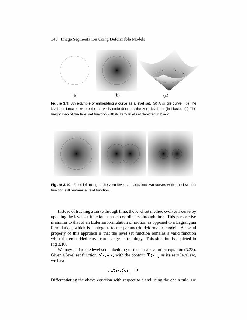
Figure 3.10: From left to right, the zero level set splits into two curves while the level set
function still remains a valid function.
Instead of tracking a curve through time, the level set method evolves a curve byupdating the level set function at fixed coordinates through time. This perspectiveis similar to that of an Eulerian formulation of motion as opposed to a Lagrangianformulation, which is analogous to the parametric deformable model. A usefulproperty of this approach is that the level set function remains a valid functionwhile the embedded curve can change its topology. This situation is depicted inFig 3.10.
We now derive the level set embedding of the curve evolution equation (3.23).Given a level set function �� �� �� with the contour ���� �� as its zero level set,we have
����� ��� �� � � �
Differentiating the above equation with respect to � and using the chain rule, we
Geometric deformable models 149
obtain
�
���� �
��
��� � � (3.24)
where � denotes the gradient of .We assume that is negative inside the zero level set and positive outside.
Accordingly, the inward unit normal to the level set curve is given by
� � ��
�� �� (3.25)
Using this fact and Eq. (3.23), we can rewrite Eq. (3.24) as
�
��� � ����� � � (3.26)
where the curvature � at the zero level set is given by
� � � ��
�� �� ��
�� � � � � �� � ��
��
� �� � ���� �
� (3.27)
The relationship between Eq. (3.23) and Eq. (3.26) provides the basis for perform-ing curve evolution using the level set method.
Three issues need to be considered in order to implement geometric deformablecontours:
1. An initial function �� �� � � �� must be constructed such that its zero levelset corresponds to the position of the initial contour. A common choice isto set �� �� �� � ��� ��, where ��� �� is the signed distance from eachgrid point to the zero level set. The computation of the signed distance for anarbitrary initial curve is expensive. Recently, Sethian and Malladi developeda method called the fast marching method, which can construct the signeddistance function in !�� ����, where � is the number of pixels. Certainsituations may arise, however, where the distance may be computed muchmore efficiently. For example, when the zero level set can be described bythe exterior boundary of the union of a collection of disks, the signed distancefunction can be computed in !��� as
���� � ����������� ��
���� � � �� �
where � � �� ��, " is the number of initial disks, and � are the centerand radius of each disk.
2. Since the evolution equation (3.26) is derived for the zero level set only, thespeed function � ���, in general, is not defined on other level sets. Hence,we need a method to extend the speed function � ��� to all of the level sets.

150 Image Segmentation Using Deformable Models
We note that the expressions for the unit normal and the curvature, however,hold for all level sets. Many approaches for such extensions have been de-veloped (see [33] for a detailed discussion on this topic). However, the levelset function that evolves using these extended speed functions can lose itsproperty of being a signed distance function, causing inaccuracy in curvatureand normal calculations. As a result, reinitialization of the level set functionto a signed distance function is often required for these schemes. Recently, amethod that does not suffer from this problem was proposed by Adalsteins-son and Sethian [61]. This method casts the speed extension problem as aboundary value problem, which can then be solved efficiently using the fastmarching method.
3. In the application of geometric contours, constant deformation is often usedto account for large-scale deformation and narrow boundary indentation andprotrusion recovery. Constant deformation, however, can cause the formationof sharp corners from an initial smooth zero level set. Once the corner isdeveloped, it is not clear how to continue the deformation, since the definitionof the normal direction becomes ambiguous. A natural way to continue thedeformation is to impose the so-called entropy condition originally proposedin the area of interface propagation by Sethian [62]. In Section 3.3.5, wedescribe an entropy satisfying numerical scheme, proposed by Osher andSethian [32], which implements geometric deformable contours.
3.3.3 Speed functions
In this section, we provide a brief overview of three examples of speed func-tions used by geometric deformable contours.
The geometric deformable contour formulation, proposed by Caselles et al. [24]and Malladi et al. [25], takes the following form:
�
��� #��� ����� � � (3.28)
where
# ��
� � ����� � ���� (3.29)
Positive �� shrinks the curve, and negative �� expands the curve. The curve evolu-tion is coupled with the image data through a multiplicative stopping term #. Thisscheme can work well for objects that have good contrast. However, when the ob-ject boundary is indistinct or has gaps, the geometric deformable contour may leakout because the multiplicative term only slows down the curve near the boundaryrather than completely stopping the curve. Once the curve passes the boundary, itwill not be pulled back to recover the correct boundary.

Geometric deformable models 151
Figure 3.11: Contour extraction of cyst form ultrasound breast image via merging multiple
initial level sets. Images courtesy of Yezzi [63], Georgia Institute of Technology.
To remedy the latter problem, Caselles et al. [26,64] and Kichenassamy et al. [63,65] used an energy minimization formulation to design the speed function. Thisleads to the following geometric deformable contour formulation:
�
��� #��� ����� ���# � � � (3.30)
Note that the resulting speed function has an extra stopping term �# � � that canpull back the contour if it passes the boundary. This term behaves in similar fashionto the Gaussian potential force in the parametric formulation. An example of usingthis type of geometrical deformable contours is shown in Fig. 3.11.
The latter formulation can still generate curves that pass through boundarygaps. Siddiqi et al. [66] partially address this problem by altering the constantspeed term through energy minimization, leading to the following geometric de-formable contour:
�
��� $�#��� ���# � � � � �#�
�
�� � �#��� � � (3.31)
In this case, the constant speed term �� in Eq. (3.30) is replaced by the secondterm, and the term �
�� � �# provides additional stopping power that can prevent
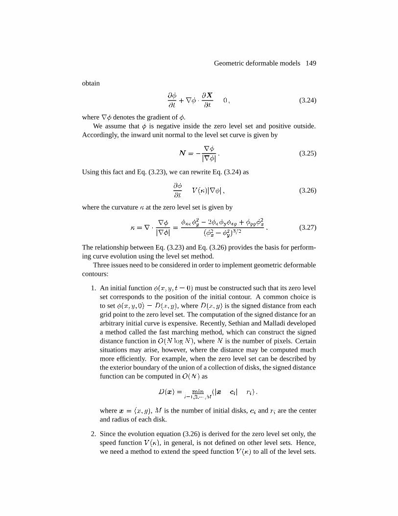
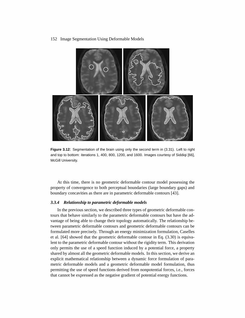
the geometrical contour from leaking through small boundary gaps. The secondterm can be used alone as the speed function for shape recovery as well. Figure 3.12shows an example of this deformable contour model. Although this model is robustto small gaps, large boundary gaps can still cause problems.
152 Image Segmentation Using Deformable Models
Figure 3.12: Segmentation of the brain using only the second term in (3.31). Left to right
and top to bottom: iterations 1, 400, 800, 1200, and 1600. Images courtesy of Siddiqi [66],
McGill University.
At this time, there is no geometric deformable contour model possessing theproperty of convergence to both perceptual boundaries (large boundary gaps) andboundary concavities as there are in parametric deformable contours [43].
3.3.4 Relationship to parametric deformable models
In the previous section, we described three types of geometric deformable con-tours that behave similarly to the parametric deformable contours but have the ad-vantage of being able to change their topology automatically. The relationship be-tween parametric deformable contours and geometric deformable contours can beformulated more precisely. Through an energy minimization formulation, Caselleset al. [64] showed that the geometric deformable contour in Eq. (3.30) is equiva-lent to the parametric deformable contour without the rigidity term. This derivationonly permits the use of a speed function induced by a potential force, a propertyshared by almost all the geometric deformable models. In this section, we derive anexplicit mathematical relationship between a dynamic force formulation of para-metric deformable models and a geometric deformable model formulation, thuspermitting the use of speed functions derived from nonpotential forces, i.e., forcesthat cannot be expressed as the negative gradient of potential energy functions.
Geometric deformable models 153
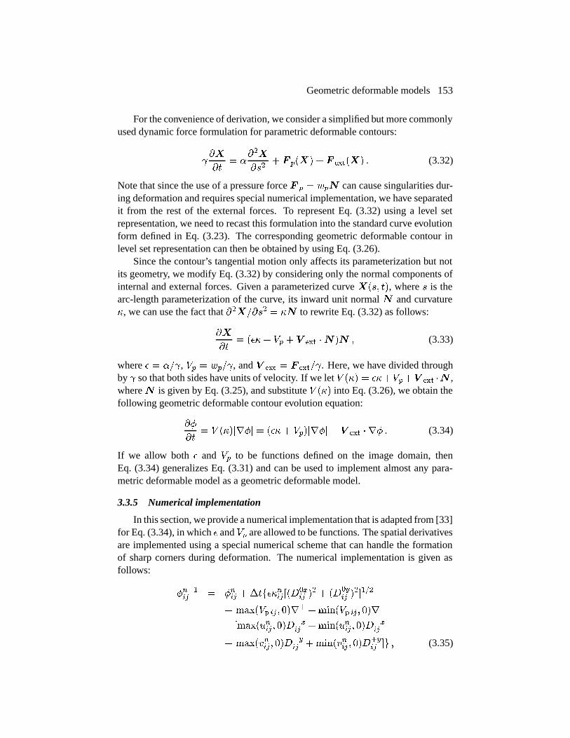
For the convenience of derivation, we consider a simplified but more commonlyused dynamic force formulation for parametric deformable contours:
���
��� �
���
���� � ���� � � ������ � (3.32)
Note that since the use of a pressure force � � � �� can cause singularities dur-ing deformation and requires special numerical implementation, we have separatedit from the rest of the external forces. To represent Eq. (3.32) using a level setrepresentation, we need to recast this formulation into the standard curve evolutionform defined in Eq. (3.23). The corresponding geometric deformable contour inlevel set representation can then be obtained by using Eq. (3.26).
Since the contour’s tangential motion only affects its parameterization but notits geometry, we modify Eq. (3.32) by considering only the normal components ofinternal and external forces. Given a parameterized curve ���� ��, where � is thearc-length parameterization of the curve, its inward unit normal � and curvature�, we can use the fact that ������� � �� to rewrite Eq. (3.32) as follows:
��
��� �%�� �� � ��� ���� � (3.33)
where % � ���, �� � ���, and ��� � � �����. Here, we have divided throughby � so that both sides have units of velocity. If we let � ��� � %����� ��� �� ,where� is given by Eq. (3.25), and substitute � ��� into Eq. (3.26), we obtain thefollowing geometric deformable contour evolution equation:
�
��� � ����� � � �%�� ����� � � ��� � � � (3.34)
If we allow both % and �� to be functions defined on the image domain, thenEq. (3.34) generalizes Eq. (3.31) and can be used to implement almost any para-metric deformable model as a geometric deformable model.
3.3.5 Numerical implementation
In this section, we provide a numerical implementation that is adapted from [33]for Eq. (3.34), in which % and �� are allowed to be functions. The spatial derivativesare implemented using a special numerical scheme that can handle the formationof sharp corners during deformation. The numerical implementation is given asfollows:
�� � � ���%�������� �
� � ����� �
��� �
� ����� � � ��� ������� � � ���
�
� ����&� � ������ �����&� � ���
��
� ���'� � ������ �����'� � ���
�� � � (3.35)
154 Image Segmentation Using Deformable Models
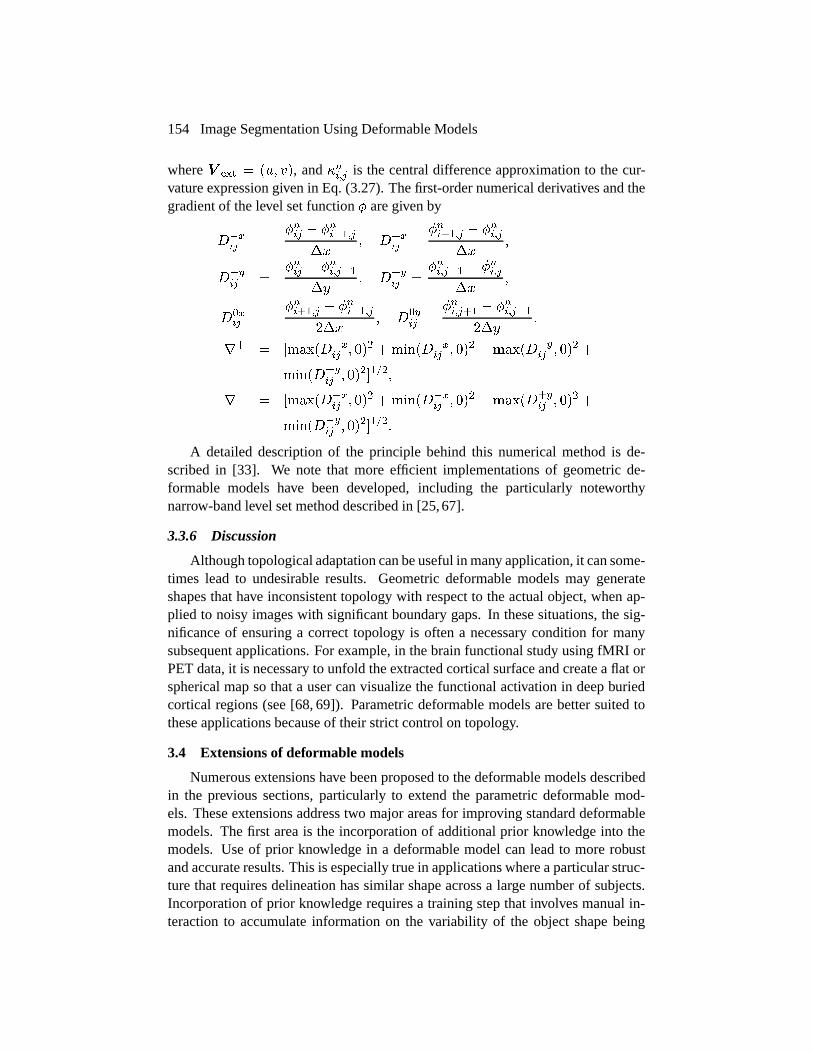
where ��� � �&� '�, and ��� is the central difference approximation to the cur-vature expression given in Eq. (3.27). The first-order numerical derivatives and thegradient of the level set function are given by
���� �
� � �����
� � �� �
��� � ���
�
���� �
� � ������
� � �� �
�� � � ���
�
���� �
��� � ������
� ���� �
�� � � �������
�
� � �������� � ��
� ������ �� � ��� �������
� � ��� �
����� �� � ��
��� ��
�� � ����� �� � ��
� ��������� � ��� ����� �
� � ��� �
�������� � ��
��� ��
A detailed description of the principle behind this numerical method is de-scribed in [33]. We note that more efficient implementations of geometric de-formable models have been developed, including the particularly noteworthynarrow-band level set method described in [25, 67].
3.3.6 Discussion
Although topological adaptation can be useful in many application, it can some-times lead to undesirable results. Geometric deformable models may generateshapes that have inconsistent topology with respect to the actual object, when ap-plied to noisy images with significant boundary gaps. In these situations, the sig-nificance of ensuring a correct topology is often a necessary condition for manysubsequent applications. For example, in the brain functional study using fMRI orPET data, it is necessary to unfold the extracted cortical surface and create a flat orspherical map so that a user can visualize the functional activation in deep buriedcortical regions (see [68, 69]). Parametric deformable models are better suited tothese applications because of their strict control on topology.
3.4 Extensions of deformable models
Numerous extensions have been proposed to the deformable models describedin the previous sections, particularly to extend the parametric deformable mod-els. These extensions address two major areas for improving standard deformablemodels. The first area is the incorporation of additional prior knowledge into themodels. Use of prior knowledge in a deformable model can lead to more robustand accurate results. This is especially true in applications where a particular struc-ture that requires delineation has similar shape across a large number of subjects.Incorporation of prior knowledge requires a training step that involves manual in-teraction to accumulate information on the variability of the object shape being

Extensions of deformable models 155
delineated. This information is then used to constrain the actual deformation of thecontour or surface to extract shapes consistent with the training data.
The second area that has been addressed by various extensions of deformablemodels is in modeling global shape properties. Traditional parametric and geo-metric deformable models are local models — contours or surfaces are assumedto be locally smooth. Global properties such as orientation and size are not ex-plicitly modeled. Modeling of global properties can provide greater robustness toinitialization. Furthermore, global properties are important in object recognitionand image interpretation applications because they can be characterized using onlya few parameters. Note that although prior knowledge and global shape propertiesare distinct concepts, they are often used in conjunction with one another. Globalproperties tend to be much more stable than local properties. Therefore, if informa-tion about the global properties is known a priori, it can be used to greatly improvethe performance of the deformable model.
In this section, we review several extensions of deformable models that useprior knowledge and/or global shape properties. We focus on revealing the funda-mental principles of each extension and refer the reader to the cited literature for afull treatment of the topic.
3.4.1 Deformable Fourier models
In standard deformable models, a direct parameterization is typically utilizedfor representing curves and surfaces. Staib and Duncan [70] have proposed usinga Fourier representation for parameterizing deformable contours and surfaces. AFourier representation for a closed contour is expressed as
���� �
������ ���
��
�(�#�
��
�����
�(� )�#� ��
� ���� �*+���� �*+�
�� (3.36)
where (�� #�� (�� )�� #�� ��� � � � are Fourier coefficients. The Fourier coefficients of���� are computed by
(� ��
�*
� �
�
������
(� ��
*
� �
�
���� ��� �*+� ��
)� ��
*
� �
�
���� ��� �*+� �� �
and the coefficients of � ��� are computed in analogous fashion. Open contourscan also be parameterized using a straightforward modification of Eq. (3.36), asdescribed in [70].
The advantages of the Fourier representation are that a compact representationof smooth shapes can be obtained by truncating the series and that a geometric

156 Image Segmentation Using Deformable Models
description of the shape can be derived to characterize global shape properties.From Eq. (3.36), the coefficients (� and #� define the translation of the contour.Each subsequent term in the series expansion follows the parametric form of anellipse. It is possible to map the coefficients to a parameter set that describes theobject shape in terms of standard properties of ellipses [70]. Furthermore, likethe Fourier coefficients, these parameters follow a scale ordering, where low indexparameters describe global properties and higher indexed parameters describe morelocal deformations.
Figure 3.13: Segmenting the corpus callosum from an MR midbrain sagittal image using
a deformable Fourier model. Top left: MR image (146�106). Top right: positive magnitude
of the Laplacian of the Gaussian (� � ���). Bottom left: initial contour (six harmonics).
Bottom right: final contour on the corpus callosum of the brain. Images courtesy of Staib
and Duncan [70], Yale University.
Staib and Duncan apply a Bayesian approach to incorporating prior informa-tion into their model. A prior probability function is defined by first manually orsemi-automatically delineating structures of the same class as the structure to beextracted. Next, these structures are parameterized using the Fourier coefficients,or using the converted parameter set based on ellipses. Mean and variance statisticsare finally computed for each of the parameters.
Assuming independence between the parameters, the multivariate Gaussian
Extensions of deformable models 157
prior probability function is given by
���� �����
��*��
,�
��������
���� � (3.37)
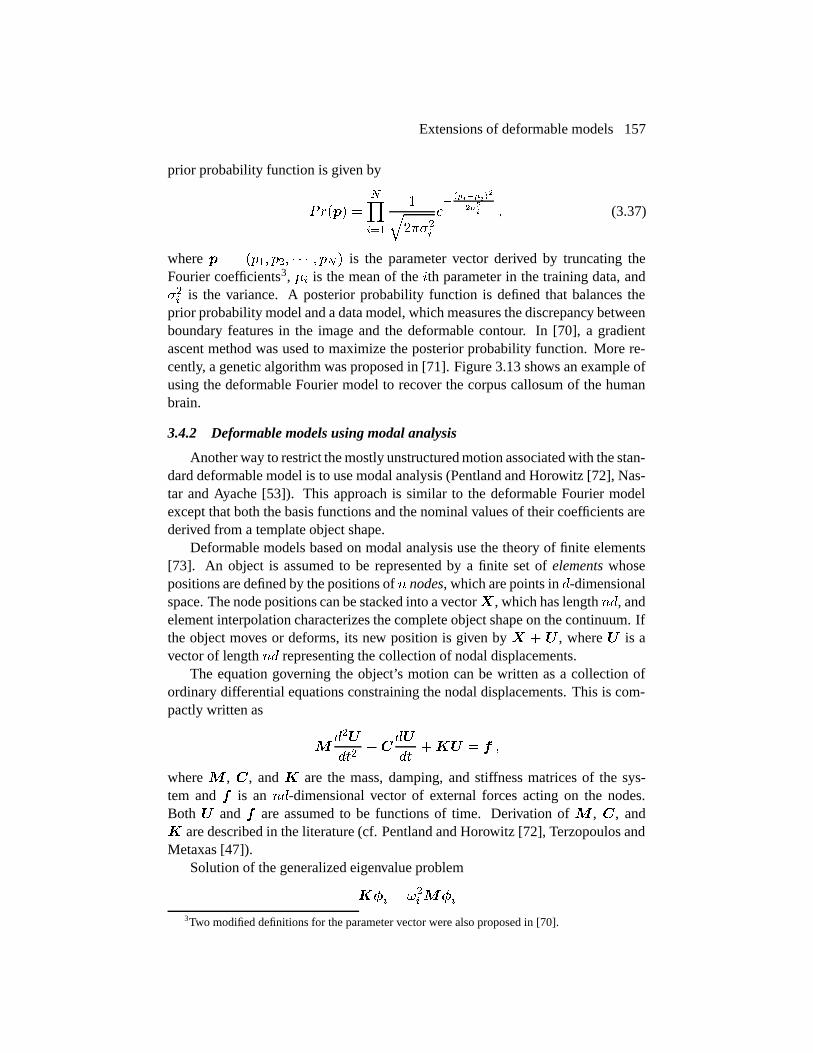
where � � �-�� -�� � � � � -� � is the parameter vector derived by truncating theFourier coefficients3, � is the mean of the �th parameter in the training data, and�� is the variance. A posterior probability function is defined that balances theprior probability model and a data model, which measures the discrepancy betweenboundary features in the image and the deformable contour. In [70], a gradientascent method was used to maximize the posterior probability function. More re-cently, a genetic algorithm was proposed in [71]. Figure 3.13 shows an example ofusing the deformable Fourier model to recover the corpus callosum of the humanbrain.
3.4.2 Deformable models using modal analysis
Another way to restrict the mostly unstructured motion associated with the stan-dard deformable model is to use modal analysis (Pentland and Horowitz [72], Nas-tar and Ayache [53]). This approach is similar to the deformable Fourier modelexcept that both the basis functions and the nominal values of their coefficients arederived from a template object shape.
Deformable models based on modal analysis use the theory of finite elements[73]. An object is assumed to be represented by a finite set of elements whosepositions are defined by the positions of � nodes, which are points in �-dimensionalspace. The node positions can be stacked into a vector� , which has length ��, andelement interpolation characterizes the complete object shape on the continuum. Ifthe object moves or deforms, its new position is given by � � � , where � is avector of length �� representing the collection of nodal displacements.
The equation governing the object’s motion can be written as a collection ofordinary differential equations constraining the nodal displacements. This is com-pactly written as
����
����
��
����� � � �
where � , , and � are the mass, damping, and stiffness matrices of the sys-tem and � is an ��-dimensional vector of external forces acting on the nodes.Both � and � are assumed to be functions of time. Derivation of � , , and� are described in the literature (cf. Pentland and Horowitz [72], Terzopoulos andMetaxas [47]).
Solution of the generalized eigenvalue problem
�� � .���
3Two modified definitions for the parameter vector were also proposed in [70].
158 Image Segmentation Using Deformable Models
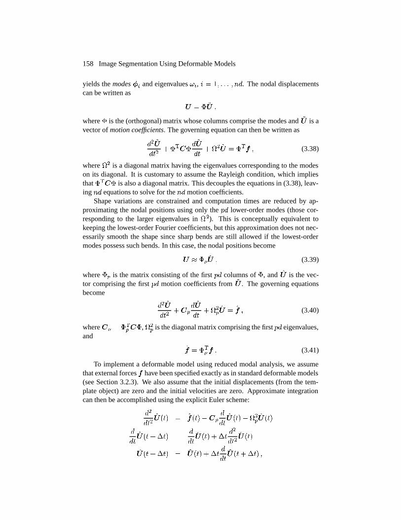
yields the modes � and eigenvalues ., � � �� � � � � ��. The nodal displacementscan be written as
� � � �� �
where � is the (orthogonal) matrix whose columns comprise the modes and �� is avector of motion coefficients. The governing equation can then be written as
�� ��
���� �� �
� ��
��� �� �� � ��� � (3.38)
where �� is a diagonal matrix having the eigenvalues corresponding to the modeson its diagonal. It is customary to assume the Rayleigh condition, which impliesthat �� � is also a diagonal matrix. This decouples the equations in (3.38), leav-ing �� equations to solve for the �� motion coefficients.
Shape variations are constrained and computation times are reduced by ap-proximating the nodal positions using only the -� lower-order modes (those cor-responding to the larger eigenvalues in ��). This is conceptually equivalent tokeeping the lowest-order Fourier coefficients, but this approximation does not nec-essarily smooth the shape since sharp bends are still allowed if the lowest-ordermodes possess such bends. In this case, the nodal positions become
� ���� � (3.39)
where �� is the matrix consisting of the first -� columns of �, and �� is the vec-tor comprising the first -� motion coefficients from �� . The governing equationsbecome
�� ��
���� �
� ��
��� ��
��� � �� � (3.40)
where � � ��� �, ��
� is the diagonal matrix comprising the first -� eigenvalues,and
�� � ��� � � (3.41)
To implement a deformable model using reduced modal analysis, we assumethat external forces � have been specified exactly as in standard deformable models(see Section 3.2.3). We also assume that the initial displacements (from the tem-plate object) are zero and the initial velocities are zero. Approximate integrationcan then be accomplished using the explicit Euler scheme:
��
�������� � ������ �
�
�������� ��
������
�
���������� �
�
������� � ��
��
��������
�������� � ����� � ���
���������� �
Extensions of deformable models 159
where �� is a time step that must be chosen small enough for convergence and goodaccuracy. The nodal displacements are given by Eq. (3.39) and the nodal positionsare given by � � � . Using this information, the vector of external forces can berecomputed from the image data after each time step. Solution of the explicit Eulerscheme equations is particularly easy because the equations are decoupled, and itis very fast because only the -� retained modes need be computed.
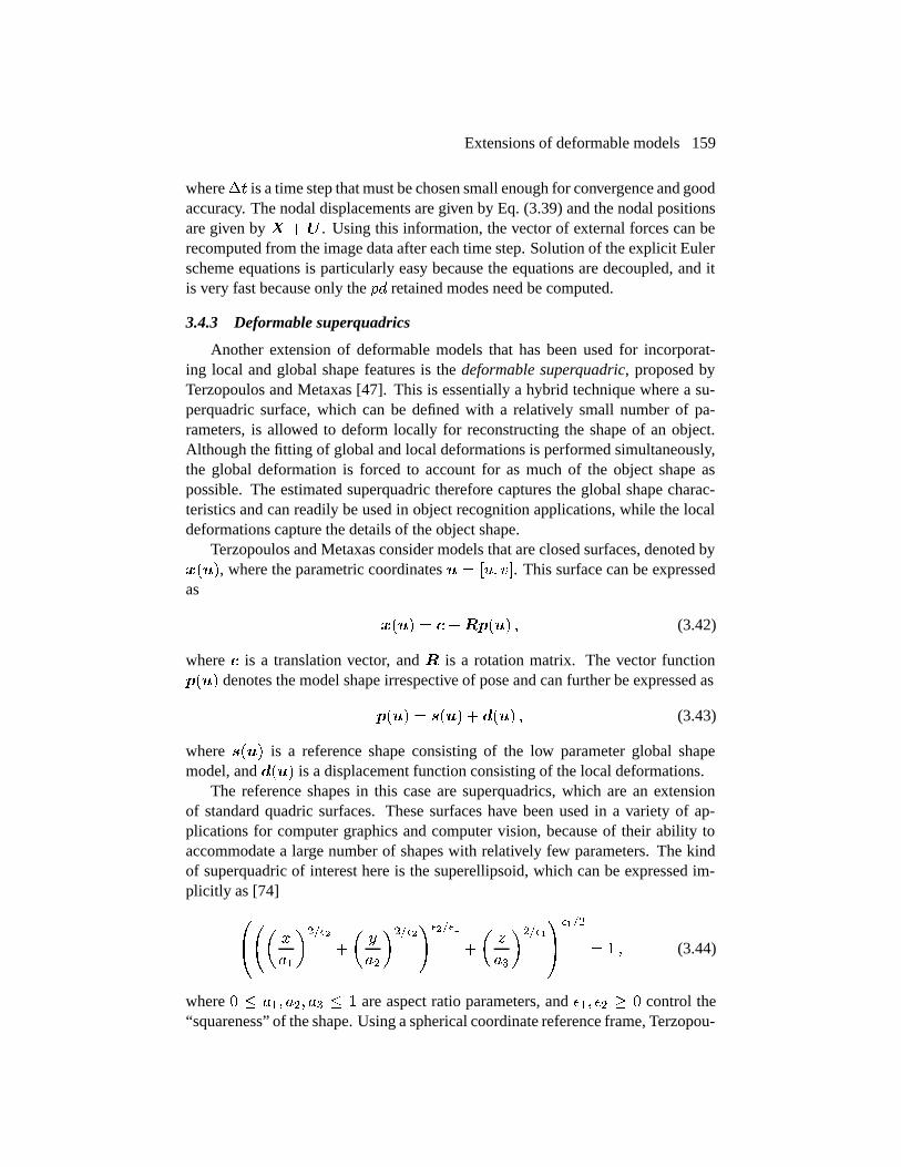
3.4.3 Deformable superquadrics
Another extension of deformable models that has been used for incorporat-ing local and global shape features is the deformable superquadric, proposed byTerzopoulos and Metaxas [47]. This is essentially a hybrid technique where a su-perquadric surface, which can be defined with a relatively small number of pa-rameters, is allowed to deform locally for reconstructing the shape of an object.Although the fitting of global and local deformations is performed simultaneously,the global deformation is forced to account for as much of the object shape aspossible. The estimated superquadric therefore captures the global shape charac-teristics and can readily be used in object recognition applications, while the localdeformations capture the details of the object shape.
Terzopoulos and Metaxas consider models that are closed surfaces, denoted by����, where the parametric coordinates � � �&� '�. This surface can be expressedas
���� � ������ � (3.42)
where is a translation vector, and � is a rotation matrix. The vector function���� denotes the model shape irrespective of pose and can further be expressed as
���� � ���� � ���� � (3.43)
where ���� is a reference shape consisting of the low parameter global shapemodel, and ���� is a displacement function consisting of the local deformations.
The reference shapes in this case are superquadrics, which are an extensionof standard quadric surfaces. These surfaces have been used in a variety of ap-plications for computer graphics and computer vision, because of their ability toaccommodate a large number of shapes with relatively few parameters. The kindof superquadric of interest here is the superellipsoid, which can be expressed im-plicitly as [74]
���
(�
�� ��
�
��
(�
�� �� �� ��
�
�/
(�
�� ��
��
�� �
� � � (3.44)
where � � (�� (�� (� � � are aspect ratio parameters, and %�� %� � � control the“squareness” of the shape. Using a spherical coordinate reference frame, Terzopou-
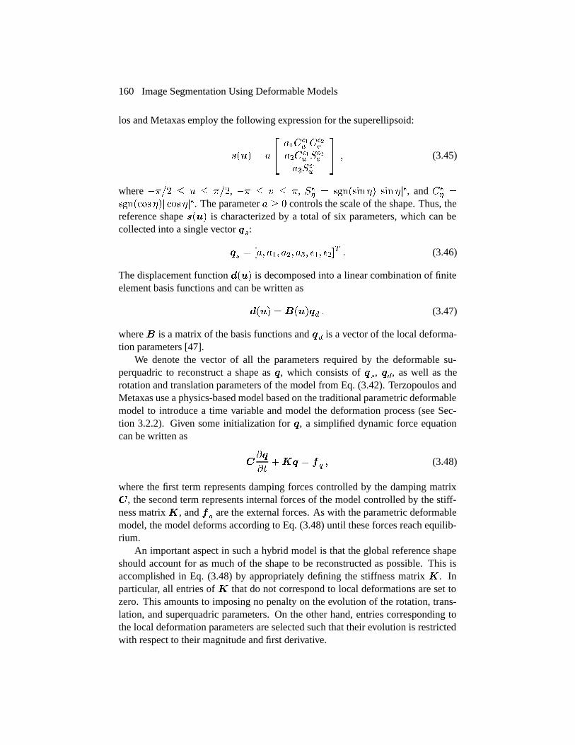
160 Image Segmentation Using Deformable Models
los and Metaxas employ the following expression for the superellipsoid:
���� � (
�� (�0
��� 0
���
(�0��� 1
���
(�1���
�� � (3.45)
where �*�� � & � *��, �* � ' � *, 1�� � ������� 2�� ��� 2��, and 0�
� �������� 2�� ��� 2��. The parameter ( � � controls the scale of the shape. Thus, thereference shape ���� is characterized by a total of six parameters, which can becollected into a single vector ��:
�� � �(� (�� (�� (�� %�� %��� � (3.46)
The displacement function ���� is decomposed into a linear combination of finiteelement basis functions and can be written as
���� � ������ � (3.47)
where � is a matrix of the basis functions and �� is a vector of the local deforma-tion parameters [47].
We denote the vector of all the parameters required by the deformable su-perquadric to reconstruct a shape as �, which consists of ��, ��, as well as therotation and translation parameters of the model from Eq. (3.42). Terzopoulos andMetaxas use a physics-based model based on the traditional parametric deformablemodel to introduce a time variable and model the deformation process (see Sec-tion 3.2.2). Given some initialization for �, a simplified dynamic force equationcan be written as
��
����� � � � � (3.48)
where the first term represents damping forces controlled by the damping matrix , the second term represents internal forces of the model controlled by the stiff-ness matrix �, and � � are the external forces. As with the parametric deformablemodel, the model deforms according to Eq. (3.48) until these forces reach equilib-rium.
An important aspect in such a hybrid model is that the global reference shapeshould account for as much of the shape to be reconstructed as possible. This isaccomplished in Eq. (3.48) by appropriately defining the stiffness matrix �. Inparticular, all entries of � that do not correspond to local deformations are set tozero. This amounts to imposing no penalty on the evolution of the rotation, trans-lation, and superquadric parameters. On the other hand, entries corresponding tothe local deformation parameters are selected such that their evolution is restrictedwith respect to their magnitude and first derivative.
Extensions of deformable models 161
As with traditional parametric deformable models, the deformable superquadricis also well suited to motion estimation tasks, as is described in [75]. For this rea-son, a popular application of models based on superquadrics has been in cardiacimaging [74], where the simple shape of the heart can be readily modeled by asuperellipsoid. The deformable superquadric model has been extended by Vemuriand Radisavljevic [76], who employed a wavelet parameterization of the local de-formation process. The multiresolution nature of the wavelet decomposition allowsfor a smooth transition between the global superquadric and the local descriptors.They also present a method utilizing training data for obtaining a prior model ofthe global parameters. The deformable superquadric model has also been adaptedto multilevel shape representation [77].
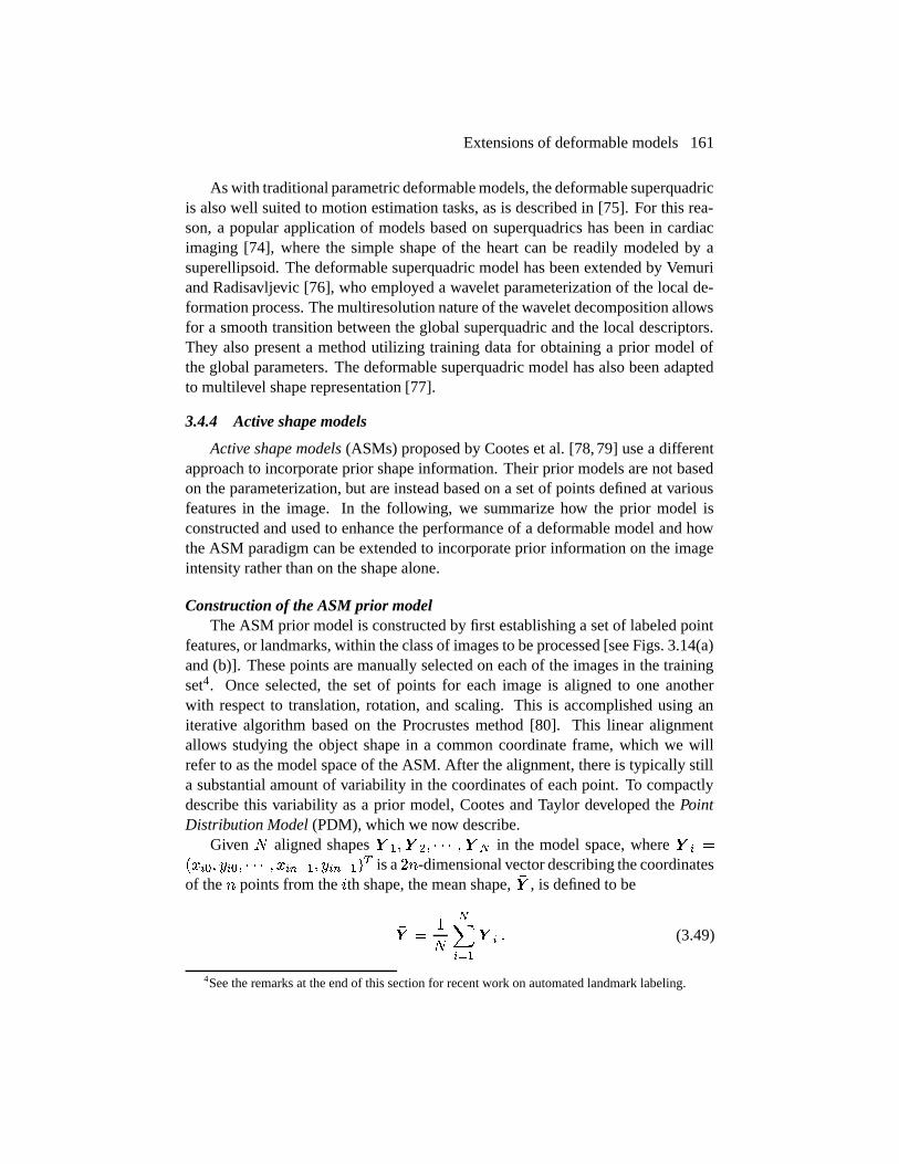
3.4.4 Active shape models
Active shape models (ASMs) proposed by Cootes et al. [78, 79] use a differentapproach to incorporate prior shape information. Their prior models are not basedon the parameterization, but are instead based on a set of points defined at variousfeatures in the image. In the following, we summarize how the prior model isconstructed and used to enhance the performance of a deformable model and howthe ASM paradigm can be extended to incorporate prior information on the imageintensity rather than on the shape alone.
Construction of the ASM prior modelThe ASM prior model is constructed by first establishing a set of labeled point
features, or landmarks, within the class of images to be processed [see Figs. 3.14(a)and (b)]. These points are manually selected on each of the images in the trainingset4. Once selected, the set of points for each image is aligned to one anotherwith respect to translation, rotation, and scaling. This is accomplished using aniterative algorithm based on the Procrustes method [80]. This linear alignmentallows studying the object shape in a common coordinate frame, which we willrefer to as the model space of the ASM. After the alignment, there is typically stilla substantial amount of variability in the coordinates of each point. To compactlydescribe this variability as a prior model, Cootes and Taylor developed the PointDistribution Model (PDM), which we now describe.
Given � aligned shapes � ��� �� � � � �� � in the model space, where � ���� ��� � � � � ��� ����� is a ��-dimensional vector describing the coordinatesof the � points from the �th shape, the mean shape, �� , is defined to be
�� ��
�
����
� � (3.49)
4See the remarks at the end of this section for recent work on automated landmark labeling.

162 Image Segmentation Using Deformable Models
(a) (b)
(c)
Figure 3.14: An example of constructing Point Distribution Models. (a) An MR brain im-
age, transaxial slice, with 114 landmark points of deep neuroanatomical structures super-
imposed. (b) A 114-point shape model of 10 brain structures. (c) Effect of simultaneously
varying the model’s parameters corresponding to the first two largest eigenvalues (on a
bi-dimensional grid). Images courtesy of Duta and Sonka [81], The University of Iowa.

Extensions of deformable models 163
A covariance matrix, �, is computed by
� ��
� � �
����
�� � �� ��� � �� �� � (3.50)
The eigenvectors corresponding to the largest eigenvalues of the covariance ma-trix describe the most significant modes of variation. Because almost all of thevariability in the model can be described using these eigenvectors, only � sucheigenvectors are selected to characterize the entire variability of the training set.Note that in general, � is significantly smaller than the number of points in themodel.
Using a principal component analysis (PCA), any shape � in the training setcan be approximated by
� �� � �� � (3.51)
where � � ����� � � ���� is the matrix of the first � eigenvectors, and � ��)�)� � � � )��� is a vector of weights, referred to as the shape parameters. Thechange of shape can be made by varying � accordingly. Limits on the values of� are imposed to constrain the actual amount of deviation from the mean shape.Figure 3.14(c) shows a collection of shapes generated for several subcortical struc-tures from similar transaxial MR brain images by using the two most significanteigenvectors.
Model fitting procedureThe key idea of ASMs is to constrain the behavior of deformable models us-
ing the PDM obtained as described in the previous section (cf. [79, 81, 82]). Ateach iteration, a standard deformation of the parametric deformable model is ap-proximated by adjusting both the pose (translation, rotation, and scale) parametersand the shape parameters of the model instance. Thus, only deformations that pro-duce shapes similar to those in the training set are allowed. The iteration stopswhen changes in both the pose and shape parameters are insignificant. Figure 3.15shows an example of using active shape models to extract the heart wall from anultrasound image.
Let us denote the position of the model instance at the beginning of a de-formation step as � � ���� ��� � � � ����� ����
� , and the required deforma-tion computed from both internal and external forces as a displacement vector�� � ����� ���� � � � � ����� �����
� . Then the position of the model instance,� , can be compactly represented by its pose and shape parameters, i.e.,
� � �� � ��� and (3.52)
� � "��� 3��� � ��� � (3.53)

164 Image Segmentation Using Deformable Models
(a) (b)
(c) (d)
Figure 3.15: An example of Active Shape Models. (a) An echocardiogram image. (b) The
initial position of the heart chamber boundary model. The location of the model after (c) 80
and (d) 200 iterations. Images courtesy of Cootes et al. [79], The University of Manchester.
where � is the scaling factor, 3 is the rotation angle, "��� 3��� � is a linear transfor-mation that performs scaling and rotation on � , and � � � ���� ��� is the centerof the model instance.
First, a global fit is performed by adjusting the pose parameters so that the gen-erated model instance aligns best with the expected model instance� � �� . Theproper pose parameter adjustments, ��, �3, and �� �, can be estimated efficientlyusing a standard least-squares approach (see [79] for details).
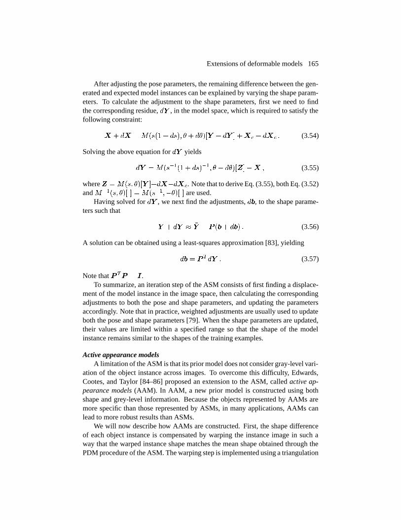
Extensions of deformable models 165
After adjusting the pose parameters, the remaining difference between the gen-erated and expected model instances can be explained by varying the shape param-eters. To calculate the adjustment to the shape parameters, first we need to findthe corresponding residue, �� , in the model space, which is required to satisfy thefollowing constraint:
� � �� � "���� � ���� 3 � �3��� � �� � ��� � ��� � (3.54)
Solving the above equation for �� yields
�� � "������ � ������ 3 � �3������ � (3.55)
where� � "��� 3��� ��������. Note that to derive Eq. (3.55), both Eq. (3.52)and "����� 3�� � � "������3�� � are used.
Having solved for �� , we next find the adjustments, ��, to the shape parame-ters such that
� � �� �� � � ��� ��� � (3.56)
A solution can be obtained using a least-squares approximation [83], yielding
�� � � ��� � (3.57)
Note that � �� � � .To summarize, an iteration step of the ASM consists of first finding a displace-
ment of the model instance in the image space, then calculating the correspondingadjustments to both the pose and shape parameters, and updating the parametersaccordingly. Note that in practice, weighted adjustments are usually used to updateboth the pose and shape parameters [79]. When the shape parameters are updated,their values are limited within a specified range so that the shape of the modelinstance remains similar to the shapes of the training examples.
Active appearance modelsA limitation of the ASM is that its prior model does not consider gray-level vari-
ation of the object instance across images. To overcome this difficulty, Edwards,Cootes, and Taylor [84–86] proposed an extension to the ASM, called active ap-pearance models (AAM). In AAM, a new prior model is constructed using bothshape and grey-level information. Because the objects represented by AAMs aremore specific than those represented by ASMs, in many applications, AAMs canlead to more robust results than ASMs.
We will now describe how AAMs are constructed. First, the shape differenceof each object instance is compensated by warping the instance image in such away that the warped instance shape matches the mean shape obtained through thePDM procedure of the ASM. The warping step is implemented using a triangulation
166 Image Segmentation Using Deformable Models
algorithm (see [87]). The resulting shape-normalized images can then be used toanalyze grey-level variations seen from various example images.
Next, a PCA is applied to the shape-normalized images, yielding a linear modelthat characterizes the grey-level variation, i.e.,
� � �� � � ��� � (3.58)
where �� is the mean normalized gray-level vector, � � is a matrix consisting ofsignificant modes of gray-level variations, and �� is the gray-level parameters thatweight the contribution from different modes of gray-level variations in � �. Asdescribed previously in Eq. (3.52), the instance shape is given by
� � �� � � ��� � (3.59)
Here, for consistency with Eq. (3.58), � � and �� are used to denote the significantmodes of shape variation and the shape parameters, respectively. Thus, given anyinstance image of the object of interest, its shape and gray-level pattern can berepresented compactly using the vectors �� and ��.
Because the shape and grey-level parameters may be correlated, a further PCAis applied to these combined shape and grey-level vectors � � �� ���� ���
� , where� � is a diagonal matrix of weights to compensate the difference in units betweenthe shape and grey-level parameters. The PCA yields another linear model
� � � �
���
��
� � (3.60)
where � is a set of orthogonal modes, 4� and 4� are the corresponding submatri-ces for the shape and gray-level parameters, respectively, and is referred to as theappearance parameters that regulate the variations of both the shape and gray-levelpattern of the model.
The final representation of the shape and graylevels in terms of is given by
� � �� � � ����� �� (3.61)
� � �� � � ��� � (3.62)
Despite the fact that the number of the appearance parameters is less than the totalnumber of the parameters in the original gray-level vector, matching the appearancemodel to an unseen image can be a time-consuming task. In [85], Cootes, Edwards,and Taylor proposed a fast matching algorithm that first learns a linear relationshipbetween matching errors and desired parameter adjustments from training exam-ples, then uses this information to predict the parameter adjustments in the realmatching process.
RemarksIn addition to the AAM extension to the ASM, there are many other extensions.
Duta and Sonka [81] applied the ASM to segment subcortical structures from MR
Conclusion and future directions 167
brain images. They improved the overall reconstruction accuracy of the ASM al-gorithm by incorporating an outlier-detection algorithm during each deformationstep. Wang and Staib [82] incorporated an additional smoothness prior into thePDM models to allow the generation of more flexible shape instances. They refor-mulated the ASM as a Bayesian problem and solved the problem by maximizingthe a posteriori probability.
A major limitation of the ASM is the requirement to place landmarks on thetraining images. This procedure is a laborious task for annotating 2D images andbecomes even more demanding for annotating 3D images. This limitation, how-ever, has been partially alleviated by the recent automatic labeling work [88–90].
3.4.5 Other models
Additional extensions have also been proposed to use global shape informationor prior shape information. For example, Ip and Shen [91] incorporated prior shapeinformation by using an affine transformation to align a shape template with thedeformable model and guide the model’s deformation to produce a shape consistentwith the template.
The deformable Fourier model, active shape model, and other extensions wediscussed so far are all parametric deformable models. Guo and Vemuri [92] haveproposed a framework for incorporating global shape prior information into ge-ometric deformable models. Like the deformable superquadric, their hybrid ge-ometric deformable model uses a combination of an underlying, low parameter,generator shape that is allowed to evolve. Their model thus retains the advantagesof traditional geometric deformable models, such as topological adaptivity.
External forces for deformable models are typically defined from edges in theimage. Fritsch et al. [93] have developed a technique called deformable shape loci,which uses information on the medial loci or cores of the shapes to be extracted (seeSection 14.3.11). The incorporation of cores provides greater robustness to imagedisturbances such as noise and blurring than purely edge-based models. This allowstheir model to be fairly robust to initialization as well as imaging artifacts. Theyalso employed a probabilistic prior model for important shape features as well asfor the spatial relationships between these features.
3.5 Conclusion and future directions
In this chapter, we have described the fundamental formulation of both para-metric and geometric deformable models and shown that they can be used in re-covering shape boundaries. We have also derived an explicit mathematical rela-tionship between these two formulations that allows one to share the design ofexternal forces and speed functions. This may lead to new, improved deformablemodels. Finally, we give a brief overview of several important extensions of de-formable models that use application-specific prior knowledge and/or global shape
168 Image Segmentation Using Deformable Models
properties to obtain more robust and accurate results.We expect that further improvements in deformable models will be made by the
continued research in both external force and speed function design, model repre-sentation, model training and learning, and model performance validation. Anotherchallenging research direction is to develop deformable models that have a greatercontrol in topology. For example, models that can both constrain or change topol-ogy depending on the requirements of an application would be extremely useful.Promising approaches have been proposed recently, such as the work by McInerneyand Terzopoulos [94], who developed a hybrid method that maintains both implicitand explicit representation for a given model to allow more effective control of thetopology. Finally, integrating deformable models with existing medical systems,such as surgical simulation, planning, and treatment systems, can further validatethe application of deformable models in a clinical setting and may in turn stimulatethe development of better deformable models.
3.6 Further reading
Several current texts deal with deformable models. The book by Blake andYuille [95] contains an excellent collection of papers on the theory and practiceof deformable models. Application of deformable models in motion tracking iscovered in great depth in two recent books [96] by Metaxas and [97] by Blake andIsard, respectively. The book edited by Singh, Goldgolf, and Terzopoulos [98] con-sists of a valuable collection of papers on deformable models and their applicationin medical image analysis. The book by Sethian [33] on level set methods is acomprehensive resource for geometric deformable models. A recent survey paperby McInerney and Terzopoulos [99] provides an excellent source for learning theapplication of deformable models in medical image analysis.
3.7 Acknowledgments
The authors would like to thank Milan Sonka, Michael Fitzpartrick, and DavidHawkes for reading and commenting upon the draft of this chapter. The work wassupported in part by an NSF Presidential Faculty Grant (MIP93-50336) and an NIHGrant (R01NS37747).
3.8 References
[1] S. M. Larie and S. S. Abukmeil, “Brain abnormality in schizophrenia: a systematicand quantitative review of volumetric magnetic resonance imaging studies,” J. Psych.,vol. 172, pp. 110–120, 1998.
[2] P. Taylor, “Invited review: computer aids for decision-making in diagnostic radiology— a literature review,” Brit. J. Radiol., vol. 68, pp. 945–957, 1995.
[3] A. P. Zijdenbos and B. M. Dawant, “Brain segmentation and white matter lesion de-tection in MR images,” Critical Reviews in Biomedical Engineering, vol. 22, pp. 401–465, 1994.
References 169
[4] A. J. Worth, N. Makris, V. S. Caviness, and D. N. Kennedy, “Neuroanatomical seg-mentation in MRI: technological objectives,” Int’l J. Patt. Recog. Artificial Intell.,vol. 11, pp. 1161–1187, 1997.
[5] C. A. Davatzikos and J. L. Prince, “An active contour model for mapping the cortex,”IEEE Trans. Med. Imag., vol. 14, pp. 65–80, 1995.
[6] V. S. Khoo, D. P. Dearnaley, D. J. Finnigan, A. Padhani, S. F. Tanner, and M. O.Leach, “Magnetic resonance imaging (MRI): considerations and applications in ra-diotheraphy treatment planning,” Radiother. Oncol., vol. 42, pp. 1–15, 1997.
[7] H. W. Muller-Gartner, J. M. Links, J. L. Prince, R. N. Bryan, E. McVeigh, J. P. Leal,C. Davatzikos, and J. J. Frost, “Measurement of radiotracer concentration in braingray matter using positron emission tomography: MRI-based correction for partialvolume effects,” J. Cereb. Blood Flow Metab., vol. 12, pp. 571–583, 1992.
[8] N. Ayache, P. Cinquin, I. Cohen, L. Cohen, F. Leitner, and O. Monga, “Segmenta-tion of complex three-dimensional medical objects: a challenge and a requirementfor computer-assisted surgery planning and performance,” in Computer-IntegratedSurgery: Technology and Clinical Applications (R. H. Taylor, S. Lavallee, G. C. Bur-dea, and R. Mosges, eds.), pp. 59–74, MIT Press, 1996.
[9] W. E. L. Grimson, G. J. Ettinger, T. Kapur, M. E. Leventon, W. M. Wells, et al., “Uti-lizing segmented MRI data in image-guided surgery,” Int’l J. Patt. Recog. ArtificialIntell., vol. 11, pp. 1367–1397, 1997.
[10] C. Xu and J. L. Prince, “Generalized gradient vector flow external forces for activecontours,” Signal Processing — An International Journal, vol. 71, no. 2, pp. 131–139,1998.
[11] C. Xu, D. L. Pham, M. E. Rettmann, D. N. Yu, and J. L. Prince, “Reconstructionof the human cerebral cortex from magnetic resonance images,” IEEE Trans. Med.Imag., vol. 18, pp. 467–480, 1999.
[12] D. Terzopoulos, “On matching deformable models to images.” Technical Report 60,Schlumberger Palo Alto research, 1986. Reprinted in Topical Meeting on MachineVision, Technical Digest Series, Vol. 12, 1987, 160-167.
[13] M. Kass, A. Witkin, and D. Terzopoulos, “Snakes: active contour models,” Int’l J.Comp. Vis., vol. 1, no. 4, pp. 321–331, 1987.
[14] D. Terzopoulos and K. Fleischer, “Deformable models,” The Visual Computer, vol. 4,pp. 306–331, 1988.
[15] D. Terzopoulos, A. Witkin, and M. Kass, “Constraints on deformable models: recov-ering 3D shape and nonrigid motion,” Artificial Intelligence, vol. 36, no. 1, pp. 91–123, 1988.
[16] M. A. Fischler and R. A. Elschlager, “The representation and matching of pictorialstructures,” IEEE Trans. on Computers, vol. 22, no. 1, pp. 67–92, 1973.
[17] B. Widrow, “The “rubber-mask” technique,” Pattern Recognition, vol. 5, pp. 175–211, 1973.
[18] A. Blake and A. Zisserman, Visual Reconstruction. Boston: MIT Press, 1987.
170 Image Segmentation Using Deformable Models
[19] U. Grenander, Y. Chow, and D. M. Keenan, Hands: A Pattern Theoretic Study ofBiological Shapes. New York: Springer-Verlag, 1991.
[20] M. I. Miller, G. E. Christensen, Y. Amit, and U. Grenander, “Mathematical text-book of deformable neuroanatomies,” Proc. National Academy of Science, vol. 90,pp. 11944–11948, 1993.
[21] A. A. Amini, T. E. Weymouth, and R. C. Jain, “Using dynamic programming forsolving variational problems in vision,” IEEE Trans. Patt. Anal. Mach. Intell., vol. 12,no. 9, pp. 855–867, 1990.
[22] L. D. Cohen, “On active contour models and balloons,” CVGIP: Imag. Under., vol. 53,no. 2, pp. 211–218, 1991.
[23] T. McInerney and D. Terzopoulos, “A dynamic finite element surface model for seg-mentation and tracking in multidimensional medical images with application to car-diac 4D image analysis,” Comp. Med. Imag. Graph., vol. 19, no. 1, pp. 69–83, 1995.
[24] V. Caselles, F. Catte, T. Coll, and F. Dibos, “A geometric model for active contours,”Numerische Mathematik, vol. 66, pp. 1–31, 1993.
[25] R. Malladi, J. A. Sethian, and B. C. Vemuri, “Shape modeling with front propagation:a level set approach,” IEEE Trans. Patt. Anal. Mach. Intell., vol. 17, no. 2, pp. 158–175, 1995.
[26] V. Caselles, R. Kimmel, and G. Sapiro, “Geodesic active contours,” in Proc. 5th Int’lConf. Comp. Vis., pp. 694–699, 1995.
[27] R. T. Whitaker, “Volumetric deformable models: active blobs,” Tech. Rep. ECRC-94-25, European Computer-Industry Research Centre GmbH, 1994.
[28] G. Sapiro and A. Tannenbaum, “Affine invariant scale-space,” Int’l J. Comp. Vis.,vol. 11, no. 1, pp. 25–44, 1993.
[29] B. B. Kimia, A. R. Tannenbaum, and S. W. Zucker, “Shapes, shocks, and deforma-tions I: the components of two-dimensional shape and the reaction-diffusion space,”Int’l J. Comp. Vis., vol. 15, pp. 189–224, 1995.
[30] R. Kimmel, A. Amir, and A. M. Bruckstein, “Finding shortest paths on surfaces usinglevel sets propagation,” IEEE Trans. Patt. Anal. Mach. Intell., vol. 17, no. 6, pp. 635–640, 1995.
[31] L. Alvarez, F. Guichard, P. L. Lions, and J. M. Morel, “Axioms and fundamental equa-tions of image processing,” Archive for Rational Mechanics and Analysis, vol. 123,no. 3, pp. 199–257, 1993.
[32] S. Osher and J. A. Sethian, “Fronts propagating with curvature-dependent speed: al-gorithms based on Hamilton-Jacobi formulations,” J. Computational Physics, vol. 79,pp. 12–49, 1988.
[33] J. A. Sethian, Level Set Methods and Fast Marching Methods: Evolving Interfaces inComputational Geometry, Fluid Mechanics, Computer Vision, and Material Science.Cambridge, UK: Cambridge University Press, 2nd ed., 1999.

References 171
[34] I. Cohen, L. D. Cohen, and N. Ayache, “Using deformable surfaces to segment 3-D images and infer differential structures,” CVGIP: Imag. Under., vol. 56, no. 2,pp. 242–263, 1992.
[35] R. Courant and D. Hilbert, Methods of Mathematical Physics, vol. 1. New York:Interscience, 1953.
[36] J. L. Prince and C. Xu, “Nonconservative force models in active geometry,” inProc. IEEE Image and Multidimensional Signal Processing Workshop (IMDSP’98),pp. 139–142, 1998.
[37] R. Ronfard, “Region-based strategies for active contour models,” Int’l J. Comp. Vis.,vol. 13, no. 2, pp. 229–251, 1994.
[38] C. S. Poon and M. Braun, “Image segmentation by a deformable contour model in-corporating region analysis,” Phys. Med. Biol., vol. 42, pp. 1833–1841, 1997.
[39] H. Tek and B. B. Kimia, “Volumetric segmentation of medical images by three-dimensional bubbles,” Comp. Vis. Imag. Under., vol. 65, pp. 246–258, 1997.
[40] L. D. Cohen and I. Cohen, “Finite-element methods for active contour models andballoons for 2-D and 3-D images,” IEEE Trans. Patt. Anal. Mach. Intell., vol. 15,no. 11, pp. 1131–1147, 1993.
[41] P. E. Danielsson, “Euclidean distance mapping,” Comp. Graph. Imag. Proc., vol. 14,pp. 227–248, 1980.
[42] G. Borgefors, “Distance transformations in arbitrary dimensions,” Comp. Vis. Graph.Imag. Proc., vol. 27, pp. 321–345, 1984.
[43] C. Xu and J. L. Prince, “Snakes, shapes, and gradient vector flow,” IEEE Trans. Imag.Proc., vol. 7, no. 3, pp. 359–369, 1998.
[44] H. Delingette, “Simplex meshes: a general representation for 3D shape reconstruc-tion,” Tech. Rep. TR2214, INRIA, Sophia-Antipolis, France, 1994.
[45] D. MacDonald, D. Avis, and A. C. Evans, “Multiple surface identification and match-ing in magnetic resonance images,” in SPIE Proc. Visualization in Biomedical Com-puting, vol. 2359, pp. 160–169, 1994.
[46] D. J. Williams and M. Shah, “A fast algorithm for active contours and curvature esti-mation,” CVGIP: Imag. Under., vol. 55, no. 1, pp. 14–26, 1992.
[47] D. Terzopoulos and D. Metaxas, “Dynamic 3D models with local and global defor-mations: deformable superquadrics,” IEEE Trans. Patt. Anal. Mach. Intell., vol. 13,pp. 703–714, 1991.
[48] A. Gupta, L. von Kurowski, A. Singh, D. Geiger, C.-C. Liang, M.-Y. Chiu, L. P. Adler,M. Haacke, and D. L. Wilson, “Cardiac MR image segmentation using deformablemodels,” in Proc. IEEE Conf. Computers in Cardiology, pp. 747–750, 1993.
[49] H. Delingette, “Adaptive and deformable models based on simplex meshes,” in Proc.IEEE Workshop on Motion of Non-Rigid and Articulated Objects, pp. 152–157, 1994.
[50] S. Kumar and D. Goldgof, “Automatic tracking of SPAMM grid and the estimation ofdeformation parameters from cardiac MR images,” IEEE Trans. Med. Imag., vol. 13,pp. 122–132, 1994.
172 Image Segmentation Using Deformable Models
[51] D. Geiger, A. Gupta, L. A. Costa, and J. Vlontzos, “Dynamic programming for de-tecting, tracking, and matching deformable contours,” IEEE Trans. Patt. Anal. Mach.Intell., vol. 17, pp. 294–402, 1995.
[52] S. Lobregt and M. A. Viergever, “A discrete dynamic contour model,” IEEE Trans.Med. Imag., vol. 14, pp. 12–24, 1995.
[53] C. Nastar and N. Ayache, “Frequency-based nonrigid motion analysis: applicationto four dimensional medical images,” IEEE Trans. Patt. Anal. Mach. Intell., vol. 18,pp. 1067–1079, 1996.
[54] R. Durikovic, K. Kaneda, and H. Yamashita, “Dynamic contour: a texture approachand contour operations,” The Visual Computer, vol. 11, pp. 277–289, 1995.
[55] T. McInerney and D. Terzopoulos, “Topologically adaptable snakes,” in Proc. 5thInt’l Conf. Comp. Vis., pp. 840–845, 1995.
[56] B. B. Kimia, Conservation Laws and a Theory of Shape. Ph.D. thesis, McGill Centrefor Intelligent Machines, McGill University, Montreal, Canada, 1990.
[57] M. A. Grayson, “Shortening embedded curves,” Annals of Mathematics, vol. 129,pp. 71–111, 1989.
[58] J. A. Sethian, “Curvature and evolution of fronts,” Commun. Math. Phys., vol. 101,pp. 487–499, 1985.
[59] J. A. Sethian, “A review of recent numerical algorithms for hypersurfaces movingwith curvature dependent speed,” J. Differential Geometry, vol. 31, pp. 131–161,1989.
[60] G. Sapiro, “Geometric partial differential equations in image analysis: past, present,and future,” in Proc. IEEE Int’l Conf. Imag. Proc., vol. 3, pp. 1–4, 1995.
[61] D. Adalsteinsson and J. A. Sethian, “The fast construction of extension velocities inlevel set methods,” J. Computational Physics, vol. 148, pp. 2–22, 1999.
[62] J. A. Sethian, An Analysis of Flame Propagation. Ph.D. thesis, Dept. of Mathematics,University of California, Berkeley, CA, 1982.
[63] A. Yezzi, S. Kichenassamy, A. Kumar, P. Olver, and A. Tennenbaum, “A geometricsnake model for segmentation of medical imagery,” IEEE Trans. Med. Imag., vol. 16,pp. 199–209, 1997.
[64] V. Caselles, R. Kimmel, and G. Sapiro, “Geodesic active contours,” Int’l J. Comp.Vis., vol. 22, pp. 61–79, 1997.
[65] S. Kichenassamy, A. Kumar, P. Olver, A. Tennenbaum, and A. Yezzi, “Conformalcurvature flows: from phase transitions to active vision,” Arch. Rational Mech. Anal.,vol. 134, pp. 275–301, 1996.
[66] K. Siddiqi, Y. B. Lauziere, A. Tannenbaum, and S. W. Zucker, “Area and lengthminimizing flows for shape segmentation,” IEEE Trans. Imag. Proc., vol. 7, pp. 433–443, 1998.
[67] D. L. Chopp, “Computing minimal surfaces via level set curvature flow,” J. of Comp.Phys., vol. 106, pp. 77–91, 1993.
References 173
[68] P. C. Teo, G. Sapiro, and B. A. Wandell, “Creating connected representations of cor-tical gray matter for functional MRI visualization,” IEEE Trans. Med. Imag., vol. 16,pp. 852–863, 1997.
[69] C. Xu, D. L. Pham, and J. L. Prince, “Finding the brain cortex using fuzzy segmen-tation, isosurfaces, and deformable surface models,” in Proc. Information Processingin Medical Imaging (IPMI’97), pp. 399–404, 1997.
[70] L. H. Staib and J. S. Duncan, “Boundary finding with parametrically deformable mod-els,” IEEE Trans. Patt. Anal. Mach. Intell., vol. 14, no. 11, pp. 1061–1075, 1992.
[71] K. Delibasis, P. E. Undrill, and G. G. Cameron, “Designing Fourier descriptor-basedgeometric models for object interpretation in medical images using genetic algo-rithms,” Comp. Vis. Imag. Under., vol. 66, pp. 286–300, 1997.
[72] A. Pentland and B. Horowitz, “Recovery of nonrigid motion and structure,” IEEETrans. Patt. Anal. Mach. Intell., vol. 13, pp. 730–742, 1991.
[73] K. H. Huebner, E. A. Thornton, and T. G. Byrom, The Finite Element Method forEngineers. New York: John Wiley & Sons, 3rd ed., 1994.
[74] E. Bardinet, L. D. Cohen, and N. Ayache, “A parametric deformable model to fitunstructured 3D data,” Comp. Vis. Imag. Under., vol. 71, pp. 39–54, 1998.
[75] D. Metaxas and D. Terzopoulos, “Shape and nonrigid motion estimation throughphysics-based synthesis,” IEEE Trans. Patt. Anal. Mach. Intell., vol. 15, pp. 580–591,1993.
[76] B. C. Vemuri and A. Radisavljevic, “Multiresolution stochastic hybrid shape modelswith fractal priors,” ACM Trans. Graph., vol. 13, pp. 177–207, 1994.
[77] D. Metaxas, E. Koh, and N. J. Badler, “Multi-level shape representation using globaldeformations and locally adaptive finite elements,” Int’l J. Comp. Vis., vol. 25, pp. 49–61, 1997.
[78] T. F. Cootes, A. Hill, C. J. Taylor, and J. Haslam, “Use of active shape models for lo-cating structures in medical images,” Imag. Vis. Computing J., vol. 12, no. 6, pp. 355–366, 1994.
[79] T. F. Cootes, C. J. Taylor, D. H. Cooper, and J. Graham, “Active shape models – theirtraining and application,” Comp. Vis. Imag. Under., vol. 61, no. 1, pp. 38–59, 1995.
[80] J. C. Gower, “Generalized Procrustes analysis,” Psychometrika, vol. 40, pp. 33–51,1975.
[81] N. Duta and M. Sonka, “Segmentation and interpretation of MR brain images: animproved active shape model,” IEEE Trans. Med. Imag., vol. 17, pp. 1049–1062,1998.
[82] Y. Wang and L. H. Staib, “Boundary finding with correspondence using statisticalshape models,” in Proc. IEEE Conf. Comp. Vis. Patt. Recog., pp. 338–345, 1998.
[83] G. H. Golub and C. F. V. Loan, Matrix Computations. Baltimore, MD: The JohnsHopkins University Press, 3rd ed., 1996.
174 Image Segmentation Using Deformable Models
[84] G. J. Edwards, C. J. Taylor, and T. F. Cootes, “Interpreting face images using activeappearance models,” in Proc. Int’l Conf. Automatic Face Gesture Recog., pp. 300–305, 1998.
[85] T. F. Cootes, G. J. Edwards, and C. J. Taylor, “Active appearance models,” in Proc.European Conf. Comp. Vis., pp. 484–498, 1998.
[86] T. F. Cootes, C. Beeston, G. J. Edwards, and C. J. Taylor, “A unified framework foratlas matching using active appearance models,” in Proc. Information Processing inMedical Imaging (IPMI’99), pp. 323–333, 1999.
[87] G. J. Edwards, C. J. Taylor, and T. F. Cootes, “Learning to identify and track faces inimage sequences,” in Proc. British Mach. Vis. Conf., pp. 317–322, 1997.
[88] A. Hill and C. J. Taylor, “Automatic landmark identification using a new methodof non-rigid correspondence,” in Proc. Information Processing in Medical Imaging(IPMI’97), pp. 483–488, Springer-Verlag, 1997.
[89] A. C. W. Kotcheff and C. J. Taylor, “Automatic construction of eigenshape models bygenetic algorithm,” in Proc. Information Processing in Medical Imaging (IPMI’97),pp. 1–14, Springer-Verlag, 1997.
[90] N. Duta, M. Sonka, and A. K. Jain, “Learning shape models from examples usingautomatic shape clustering and Procrustes analysis,” in Proc. Information Processingin Medical Imaging (IPMI’99), pp. 370–375, 1999.
[91] H. H. S. Ip and D. Shen, “An affine-invariant active contour model (AI-snake) formodel-based segmentation,” Imag. Vis. Computing J., vol. 16, pp. 135–146, 1998.
[92] Y. Guo and B. C. Vemuri, “Hybrid geometric active models for shape recovery inmedical images,” in Proc. Information Processing in Medical Imaging (IPMI’99),pp. 112–125, 1999.
[93] D. Fritsch, S. Pizer, L. Yu, V. Johnson, and E. Chaney, “Segmentation of medical im-age objects using deformable shape loci,” in Proc. Information Processing in MedicalImaging (IPMI’97), pp. 127–140, 1997.
[94] T. McInerney, Topologically Adaptable Deformable Models for Medical Image Anal-ysis. Ph.D. thesis, Department of Computer Science, University of Toronto, 1997.
[95] A. Blake and A. Yuille, eds., Active Vision. Series: Artificial intelligence, Cambridge,Massachusetts: The MIT Press, 1992.
[96] D. N. Metaxas, Physics-Based Deformable Models. Boston: Kluwer Academic Pub-lishers, 1996.
[97] A. Blake and M. Isard, Active Contours: The Application of Techniques from Graph-ics, Vision, Control Theory and Statistics to Visual Tracking of Shapes in Motion.New York: Springer-Verlag, 1998.
[98] A. Singh, D. Goldgof, and D. Terzopoulos, Deformable models in medical imageanalysis. Los Alamitos, CA: IEEE Computer Society, 1998.
[99] T. McInerney and D. Terzopoulos, “Deformable models in medical image analysis: asurvey,” Med. Imag. Anal., vol. 1, no. 2, pp. 91–108, 1996.