Chapter 3

Hysteresis in random-fieldXY and

Heisenberg models: Mean-field theory

and simulations at zero temperature

3.1 Introduction

Random field XY and Heisenberg models provide a simple framework for exploring

the effects of quenched disorder in classical systems of continuous symmetry [59].

These models and their variants have helped in understanding a wide range of phenom-

ena including random pinning of spin and charge density waves in metals [109, 110,

111], vortex lattices in disordered type-II superconductors [112, 113], liquid crystals

in porous media [114, 115, 116, 117], and disordered ferromagnets [78, 79, 118, 119,

32

3.1. Introduction 33

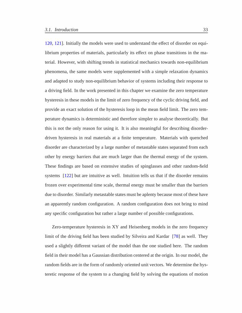
120, 121]. Initially the models were used to understand the effect of disorder on equi-

librium properties of materials, particularly its effect on phase transitions in the ma-

terial. However, with shifting trends in statistical mechanics towards non-equilibrium

phenomena, the same models were supplemented with a simple relaxation dynamics

and adapted to study non-equilibrium behavior of systems including their response to

a driving field. In the work presented in this chapter we examine the zero temperature

hysteresis in these models in the limit of zero frequency of the cyclic driving field, and

provide an exact solution of the hysteresis loop in the mean field limit. The zero tem-

perature dynamics is deterministic and therefore simpler to analyse theoretically. But

this is not the only reason for using it. It is also meaningfulfor describing disorder-

driven hysteresis in real materials at a finite temperature.Materials with quenched

disorder are characterized by a large number of metastable states separated from each

other by energy barriers that are much larger than the thermal energy of the system.

These findings are based on extensive studies of spinglassesand other random-field

systems [122] but are intuitive as well. Intuition tells us that if the disorder remains

frozen over experimental time scale, thermal energy must besmaller than the barriers

due to disorder. Similarly metastable states must be aplenty because most of these have

an apparently random configuration. A random configuration does not bring to mind

any specific configuration but rather a large number of possible configurations.

Zero-temperature hysteresis in XY and Heisenberg models inthe zero frequency

limit of the driving field has been studied by Silveira and Kardar [78] as well. They

used a slightly different variant of the model than the one studied here. The random

field in their model has a Gaussian distribution centered at the origin. In our model, the

random fields are in the form of randomly oriented unit vectors. We determine the hys-

teretic response of the system to a changing field by solving the equations of motion

3.1. Introduction 34

directly for a given initial condition. Silveira and Kardartook an indirect approach,

they recast the equations of motion into a path integral. Thepath integral is a sum over

all paths of the exponential of an action. It includes paths corresponding to different

initial conditions. They employed a method for extracting the physically relevant hys-

teretic path from among multiple solutions. We refer the reader to Ref. [78] for details.

The main object of their study is to examine critical points in the hysteretic response

of a system. They focus on a point on the hysteresis loop wherethe susceptibility of

the system diverges. If there is such a point on one half of thehysteresis loop, say in

the increasing field, there is also a symmetrically placed point on the other half of the

loop corresponding to decreasing field. These points are called non-equilibrium criti-

cal points because they are characterized by a diverging correlation length, and show

scaling of various quantities and universality of criticalexponents that is reminiscent

of equilibrium critical point phenomena. Sethna et al [63, 68, 69, 70, 76] studied the

non-equilibrium critical points on the hysteresis loop in the random field Ising model

with a Gaussian distribution of the random fields. Silveira and Kardar [78] asked the

question, if the universality class of critical hysteresisstudied by Sethna et al, would

change if we go from Ising spins to vector spins. They find no change in the case when

the critical point occurs at a non-zero value of either the applied field or the magne-

tization. However if the critical point were to occur when both the applied field and

the magnetization vanish, all components of the order parameter may become critical

simultaneously. In this case the critical point would have afull rotational symmetry of

vector spins with a new set of critical exponents.

We focus on the shape of hysteresis loop rather than the critical points on it. The

shape of hysteresis is not a universal quantity like a set of critical exponents, but

3.2. The model 35

nonetheless it is of practical interest. An exact calculation of hysteresis loop also de-

termines if there are first order jumps or critical points on the loop. The calculations

presented here bring out two rather unexpected but interesting results. In the random-

field XY model, there is a window in the value of the ferromagnetic coupling parameter

where the hysteresis loop splits into two small loops at large values of the cyclic field

but there is no hysteresis at small values of the field. This prediction of the mean-field

theory is also seen qualitatively in our simulations of the model on simple-cubic lat-

tice with nearest neighbor interactions. Similar shapes have been observed earlier in

the random-field Blume-Emery-Griffiths model for martensitic transitions [108] and

other theoretical models and experiments [118, 119, 120, 121]. But they do not ap-

pear to be known very widely. The other point is that, our mean-field theory predicts

a different kind of phase transition in random-field XY model than in random-field

Heisenberg model. This is somewhat surprising at first sight, because the two models

have the same critical behavior in the mean-field limit of therenormalization group

theory. However it is understandable if we keep in mind that our model has a different

distribution of the random field than the one used in ref. [78]. We shall return to these

issues after presenting our results.

3.2 The model

The model is defined by the Hamiltonian

H = −J∑

i, j

~Si. ~S j −∑

i

~hi . ~Si − ~h.∑

i

~Si (3.1)

3.2. The model 36

Where,~Si and~hi are n-component unit vectors located at site-i (i = 1, 2, . . .N) of a

d-dimensional lattice. In the context of magnetic systems,{~Si} are classical spins,{~hi} a

set of on-site random fields, and~h is a uniform applied field of magnitude|h|. We focus

on n = 2 (XY spins), andn = 3 (Heisenberg spins). The first sum is the ferromagnetic

exchange contribution that extends over nearest neighbor pairs (J > 0). The second

sum accounts for the interaction with random fields~hi, which stands for the disorder

present in the system. The last term is the interaction with the external driving field~h.

The random fields{~hi; |~hi | = 1} are quenched, i.e. they do not evolve in time. The spins

{ ~Si(t)} are the dynamical degrees of freedom.

At zero temperature, an initial configuration{~Si(0)} evolves in time so as to lower

the energy of the system. The evolution ends when each~Si(t) is aligned along the local

field ~fi(t) at that site. Let{~S∗i } denote a configuration at the termination of the zero-

temperature single-spin-flip dynamics. We call it a fixed-point configuration because

it remains unchanged under the dynamics. In the absence of disorder, the fixed point

has all spins parallel to each other irrespective of the starting point {~Si(0)}. This cor-

responds to the lowest energy of the system. In the presence of random fields{~hi}, the

fixed point becomes rather non trivial on two accounts. First, it may and generically

does lose its translational symmetry. Second, it is no longer independent of the starting

point. There is now a large set of fixed points each with its domain of attraction from

where it can be reached. Each of these fixed points is a local minimum of energy. A

local minimum is a stable state at zero temperature because there is no mechanism of

escape from it unless the applied field is jacked up sufficiently. It would correspond to

a metastable state under finite temperature dynamics if the thermal energy is smaller

than the barriers of disorder, but we consider zero temperature dynamics only. In equi-

librium problems with quenched disorder, one needs to know the lowest of the local

3.2. The model 37

minima. This is a difficult task analytically or computationally. Fortunately, the prob-

lem of hysteresis does not require the knowledge of the global minimum. Hysteresis

is determined by the sequence of local minima visited by the system as it tries to fol-

low a changing field. Our object is to determine this sequenceas the applied field is

cycled from−∞ to +∞ and back to−∞ in small steps. At each step, we allow the

zero-temperature dynamics as much time as it requires to come to a fixed point.

Equation (3.1) can be written as,

H = −∑

i

~fi(t). ~Si(t); ~fi(t) =J2

∑

j

~S j(t) + ~hi + ~h (3.2)

With ~fi(t) being the local field at site-i. We obtain the local minima byusing a

discrete-time dynamics that progressively lowers the energy of the system. The dy-

namics transforms a spin configuration{~Si(t)} at timet into a lower energy configura-

tion {~Si(t + 1)} at timet + 1. The fixed point of this iterative procedure corresponds to

a local minimum of the energy of the system.

The dynamics is given by the equation

~Si(t + 1) =~fi(t)

|~fi(t)|(3.3)

At each site, a new spin~Si(t + 1) is obtained that points in the direction of the

local field ~fi(t) at that site. The denominator in equation (3.3) ensures that the new spin

~Si(t + 1) has unit length;~Si(t + 1) is therefore a rotated form of~Si(t). The rotation

lowers the energy of each spin, and therefore that of the entire system. However, after

3.2. The model 38

the spins are rotated the local field changes as well. Thus therotated spin~Si(t + 1)

is generally not aligned along the new local field~fi(t + 1) at sitei. We can reduce

the energy of the system further by repeating the dynamics. Indeed, we start with a

random initial configuration{~Si(0)} and subject it to repeated applications of equation

(3.3) until a fixed point configuration{~Si(∞)} is reached. The fixed point configuration

corresponds to a local minimum of energy. The initial configuration {~Si(0)} and the

configurations along the path to the fixed point lie in the domain of attraction of the

fixed point.

For simplicity, we characterize each configuration of spinsby a single parameter

that measures the magnetization of the system along the applied field~h. We assume

that the applied field~h is along thex-axis.

3.2.1 Mean-field equation forXY spins

In the case of XY spins,~Si(t) and~hi can be completely specified by the anglesθi(t) and

αi(t) that they make with thex-axis. Thex-component of equation (3.3) gives,

cosθi(t + 1) =J∑

j cosθ j(t) + h+ cosαi

[(J∑

j cosθ j(t) + h+ cosαi)2 + (J∑

j sinθ j(t) + sinαi)2]12

(3.4)

In the mean field limit, a site-i interacts with every other site-j of the system (j , i)

with strengthJ = J0/N. Let Sxi andSy

i be the components of XY spin~Si along the x

and y axes respectively. We look for a solution of equation (3.4) in the case when the

3.2. The model 39

spins may be ordered along the x-axis, but there is no global ordering in the system in

they direction. We write,

J∑

j

Sxj (t) =

J0

N

∑

j

Sxj (t) = J0 cosθ(t) = J0m(t);

∑

j

Syj(t) = 0. (3.5)

The above equation defines a time dependent order parameter cosθ(t), or equiva-

lently a magnetizationm(t) = cosθ(t) as the average value of the component of~Si(t)

along the applied field~h. We shall mostly use the notationm(t), but keep cosθ(t) for

occasional use when convenient to do so.

Substituting from equation (3.5) into equation (3.4) we get,

cosθi(t + 1) ={J0m(t) + h} + cosαi

[1 + 2{J0m(t) + h} cosαi + {J0m(t) + h}2] 12

(3.6)

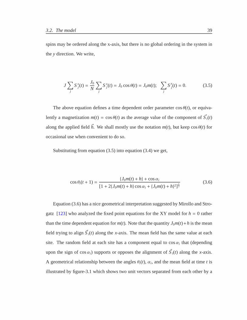
Equation (3.6) has a nice geometrical interpretation suggested by Mirollo and Stro-

gatz [123] who analyzed the fixed point equations for the XY model forh = 0 rather

than the time dependent equation form(t). Note that the quantityJ0m(t)+h is the mean

field trying to align~Si(t) along thex-axis. The mean field has the same value at each

site. The random field at each site has a component equal to cosαi that (depending

upon the sign of cosαi) supports or opposes the alignment of~Si(t) along thex-axis.

A geometrical relationship between the anglesθi(t), αi, and the mean field at timet is

illustrated by figure-3.1 which shows two unit vectors separated from each other by a

3.2. The model 40

distanceJ0m(t) + h along thex-axis, and making anglesθi(t + 1) andαi respectively

with thex-axis. From the geometry of figure-3.1, we may write

tanθi(t + 1) =sinαi

[J0m(t) + h+ cosαi](3.7)

Also, a well known identity relating the sines of the angles of a triangle to its sides

gives,

sinθi(t + 1) =sin[αi − θi(t + 1)]

[J0m(t) + h](3.8)

Equation (3.6) is the most convenient form for studying the evolution of the order

parameterm(t) but equations (3.7) and (3.8) are useful to get a geometrical picture

of the spin configuration of the system. For example, in the limit J0m(t) + h → 0,

equation (3.7) givesθi = αi as may be expected. IfJ0m(t)+ h = 1, equation (3.8) gives

θi(t + 1) = αi/2. This is expected as well. In this case the mean field as well as the

random field have unit magnitude. One acts along thex-axis and the other makes at an

angleαi with the x-axis. Therefore the resultant field aligns the spin at an angle αi/2

with thex-axis.

We obtain a recursion relation form(t + 1) = cosθ(t + 1) by averaging equation

(3.6) over all sites,

3.2. The model 41

m(t + 1) =12π

∫ 2π

0

{J0m(t) + h} + cosαi

[1 + 2{J0m(t) + h} cosαi + {J0m(t) + h}2] 12

dαi [XY model] (3.9)

3.2.2 Mean-field equation for Heisenberg spins

A similar mean field equation is obtained for Heisenberg spins. A Heisenberg spin

~Si(t) may be specified by an azimuthal angleφi(t) that the spin makes from a fixed axis

(say they-axis) in theyzplane and the polar angleθi(t) that it makes with thex-axis.

The random field~hi is also to be specified by a polar angleαi(t), and an azimuthal

angleψi(t). As in the case of the XY model, we assume that the field~h is applied in

thex-direction, and any global order in the system lies along thex-direction only.

J∑

j

Sxj (t) =

J0

N

∑

j

Sxj (t) = J0 cosθ(t) = J0m(t);

∑

j

Syj(t) = 0;

∑

j

Szj(t) = 0,(3.10)

This gives us the following mean field equation for the Heisenberg model analo-

gous to equation (3.9) for the XY model:

m(t + 1) =14π

∫ 2π

0dψi

∫ π

0

{J0m(t) + h} + cosαi

[1 + 2{J0m(t) + h} cosαi + {J0m(t) + h}2] 12

sinαidαi

[Heisenberg model]

(3.11)

3.3. Hysteresis 42

3.3 Hysteresis

We use the dynamics described above to obtain magnetizationcurves in a slowly vary-

ing cyclic field. The field is increased fromh = −∞ to h = ∞ and then decreased to

h = −∞ very slowly that the system has sufficient time to settle into a local minimum

of energy at each point. In practice we start with a large negative field when the stable

configuration of the system has all spins aligned along the negativex-axis, and then in-

crease the field in small steps till all spins point along the positivex-axis. At each step,

the field is held fixed while the system relaxes to a fixed point configuration under the

dynamics considered above. This procedure yields a line of fixed points. The graph of

the magnetizations of the fixed point configurations versus the applied field gives the

magnetization curve in increasing field. Magnetization in decreasing field is obtained

similarly. If the magnetization in decreasing field followsa different path than the one

in increasing field, the system is said to show hysteresis i.e. history-dependent effects.

We wish to know if the system characterized by Hamiltonian (3.1) exhibits hys-

teresis, and if so what is the shape of the hysteresis loop. Another question of interest

is whether there is a critical value of disorder that qualitatively separates the hysteretic

response of weakly disordered systems from that of stronglydisordered systems. The

meaning of critical disorder in this context is best explained by a reference to earlier

work of Sethna et al [68] on disorder-driven hysteresis in the random-field Ising model.

They consider a Hamiltinian similar to equation (3.1) but intheir case the spins and the

fieldsh andhi are scalar quantities; spins take the values±1 andhi is a random variable

chosen from a Gaussian distribution centered at zero and having variance equal toσ2.

Their results are based on a combination of numerical simulations and analysis, but

are quite intuitive as well. These may be summarized as follows. In the limitσ → 0

3.3. Hysteresis 43

as the applied field is increased fromh = −∞ to h = ∞ each spin and therefore the

magnetization per site flips up from−1 to+1 ath = zJwherez is the number of nearest

neighbors on the lattice. Asσ is increased, the size of the jump in the magnetization

decreases and eventually vanishes ath = hc if σ = σc. Forσ > σc, the magnetization

becomes a smooth function of the applied field. The pointh = hc, σ = σc is a nonequi-

librium critical point characterized by diverging correlation length and scaling laws

reminiscent of equilibrium critical phenomena. The parameterσ measures the width

of the random-field distribution and therefore the amount ofdisorder in the system.

The disorder is said to be critical ifσ = σc. The nonequilibrium critical point may

also be studied by fixing the disorder in the system, say by setting σ = 1 and tuning

the exchange interactionJ and the applied fieldh to the critical pointh = hc, J = Jc.

Now the magnetization curves in increasing and decreasing fields would be smooth for

J < Jc, but discontinuous forJ > Jc. The size of the discontinuity would go to zero as

J approachesJc from above.

The question is if there is a critical valueJc as we go from scalar to vector spins? In

the random-field Ising model the spins have the value+1 or -1. Therefore the bound-

aries between domains of positive and negative magnetization are sharp. The width

of the domain wall is equal to the distance between nearest neighbors on the lattice.

Vector spins can continuously change their orientation from one domain to another

over arbitrarily thick domain walls. Phase transition in a system depends on the bal-

ance between energy gained by forming a large domain, and energy lost in having to

protect it by a domain wall. The energetics of this competition in continuous spins is

very different from that in Ising spins [59]. It shows that continuous spins in random

fields cannot acquire a spontaneous long-range order below four dimensions, while the

lower critical dimension for Ising spins is two. This means that the critical hysteresis

3.3. Hysteresis 44

observed in the random-field Ising model in three dimensionsmay disappear when we

go over to vector spins. Although the focus of our work is on the shapes of hysteresis

rather than criticality, we shall return to this point afterpresenting our results.

It is useful to have a brief preview of our results before getting into details. It also

gives us an opportunity to mention some unusual aspects of hysteresis in continuous

spin systems. In our model, the disorder has a fixed magnitudeand sets the energy

scale of the system. The behavior of the model is therefore determined by the pa-

rameterJ. If J = 0, the spins decouple and there can be no hysteresis in the zero

frequency limit of the driving field. We find that the behaviorof the model for small

values ofJ is qualitatively similar to the behavior forJ = 0. This is true in the mean

field analysis as well as numerical simulations of the model on a lattice with nearest

neighbor interactions. For large values ofJ we may expect hysteresis as well as jumps

in the magnetization. The basis for this expectation is the following. LargeJ means

relatively weak disorder. Thus the spins are mostly alignedparallel to each other. As

the applied field is swept fromh = −∞ to h = ∞, we expect the majority of spins

to reverse their direction at a critical fieldh = hc. The fieldhc is determined by the

energy required to flip the least stable spin in the system that triggers a large avalanche

of flipped spins. For discrete Ising spins withz nearest neighbors,hc is of the order of

zJ in the limit of weak disorder. However, in the case of continuous spins, the least

stable spin can reverse itself by rotating smoothly along with its neighbors. In other

words, the energy barrier for magnetization reversal may bezero for continuous spins

in the strong coupling limit just as it is in the weak couplinglimit. We find that the

mean field theory predicts a non-zero value forhc but simulations based on short range

interactions on a lattice showhc→ 0 in the limit J→ ∞.

3.3. Hysteresis 45

Hysteresis in continuous spin systems at intermediate values ofJ where order and

disorder compete with each other has several unusual features. Normally if a system

shows hysteresis, the magnetization curves in increasing and decreasing fields are sep-

arated by the widest margin in the middle ath = 0. We find that there is a range of

J values where the magnetization curves for the XY model in themean field approxi-

mation overlap each other in the middle but split from each other as we go away from

h = 0 in either direction. Numerical simulations of the XY modelshow a qualitatively

similar behavior although there are significant differences between simulations and the

predictions of the mean field theory. Broadly speaking, discontinuities in the magne-

tization curves predicted by the mean field theory appear to be absent in simulations.

The mean field theory of hysteresis in the Heisenberg model has an unusual feature as

well. Usually the mean field solution is determined by the intersection of a straight line

with anS-shaped curve. In this case the mid portion of theS-shaped curve is a straight

line itself. This gives rise to some interesting effects that are seen in corresponding

simulations as well. In the following, we examine these issues in detail.

3.3.1 XY model

It is instructive to look at the mean field dynamics of the XY model numerically before

presenting the analytic solution. Let us set the applied field equal to zero (h = 0), start

with an arbitrary initial state characterized by magnetization m0, and iterate equation

(3.9) until a fixed point is reached. The results are shown in figure-3.2. We find two

critical values ofJ: Jc1 ≈ 1.489, andJc2 = 2. These values characterize discontinuities

in the fixed point behavior in increasing and decreasingJ respectively as described

below.

3.3. Hysteresis 46

The blue curve in figure-3.2 shows magnetization of fixed points of equation (3.9)

for increasingJ. We start withJ = 0, and increaseJ in small steps of∆J. At each value

of J, the magnetizationm(J−∆J) of the previous fixed point is used as a starting point

for the iteration of equations. The precise value of∆J is unimportant. We have chosen a

value of∆J that is small enough so that the line of fixed points appears asa continuous

curve on the scale of figure-3.2. For increasingJ, the fixed point magnetizationm

is zero in the range 0≤ J < Jc2. At J = Jc2, it jumps tom ≈ .92, and follows

the blue curve asJ is increased further. The return path in decreasingJ is identical

with the blue curve up toJ ≥ Jc2, but there is no discontinuity in the return path at

J = Jc2. It continues smoothly along the green curve up toJ = Jc1 at which point it

jumps down to zero and remains zero for 0≤ J < Jc1. The red curve shows a set of

unstable fixed points in the rangeJc1 ≤ J ≤ Jc2. An unstable fixed point is not realized

under iterations of equation (3.9) because its domain of attraction is zero. However,

for a fixedJ, the magnetizationmu of the unstable fixed point separates the domains of

attraction of the two stable fixed points at the same value ofJ. If the magnetization of

the starting statem0 is less thanmu, the equations iterate to the fixed point associated

with increasingJ. If m0 > mu the equations iterate to the corresponding fixed point for

decreasingJ. The reason for the existence of two stable and one unstable fixed point

in the rangeJc1 ≤ J ≤ Jc2 may be understood analytically as follows. We define,

f (ut) =12π

∫ 2π

0

ut + cosαi

[1 + 2ut cosαi + u2t ]

12

dαi whereut = J0m(t) + h (3.12)

The quantityf (ut) can be written in terms of complete elliptic integrals of the first

and second kinds [123]:

3.3. Hysteresis 47

f (ut) =1πut

[

(ut − 1)K

(

2√

ut

1+ ut

)

+ (ut + 1)E

(

2√

ut

1+ ut

)]

(3.13)

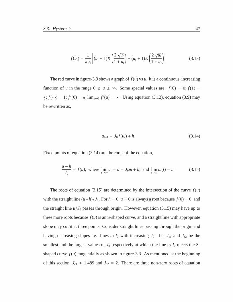
The red curve in figure-3.3 shows a graph off (u) vsu. It is a continuous, increasing

function of u in the range 0≤ u ≤ ∞. Some special values are:f (0) = 0; f (1) =

2π; f (∞) = 1; f ′(0) = 1

2; limu→1 f ′(u) = ∞. Using equation (3.12), equation (3.9) may

be rewritten as,

ut+1 = J0 f (ut) + h (3.14)

Fixed points of equation (3.14) are the roots of the equation,

u− hJ0= f (u); where lim

t→∞ut = u = J0m+ h; and lim

t→∞m(t) = m (3.15)

The roots of equation (3.15) are determined by the intersection of the curvef (u)

with the straight line (u−h)/J0. Forh = 0,u = 0 is always a root becausef (0) = 0, and

the straight lineu/J0 passes through origin. However, equation (3.15) may have upto

three more roots becausef (u) is an S-shaped curve, and a straight line with appropriate

slope may cut it at three points. Consider straight lines passing through the origin and

having decreasing slopes i.e. linesu/J0 with increasingJ0. Let Jc1 and Jc2 be the

smallest and the largest values ofJ0 respectively at which the lineu/J0 meets the S-

shaped curvef (u) tangentially as shown in figure-3.3. As mentioned at the beginning

of this section,Jc1 ≈ 1.489 andJc2 = 2. There are three non-zero roots of equation

3.3. Hysteresis 48

(3.15) in the rangeJc1 ≤ J0 ≤ Jc2, and only one non-zero root forJ0 > Jc2. Which of

these roots is actually realized by the dynamics is determined by the starting pointu0

used in iterating equation (3.14). The stability of a root can be checked by analyzing

equation (3.14) in the neighborhood of its fixed point [123]. However, the full equation

is necessary to determine the domain of attraction of a stable fixed point.

Next we consider equation (3.14) for a fixed value ofJ0 but in a varying fieldh.

Starting from a sufficiently large negative fieldh = hmin where the stable configuration

has most spins pointing along the negativex-axis, the field is increased in small steps

∆h to h = hmax where most spins point along the positivex-axis. Figure-3.4 shows the

fixed point magnetizationmas the field is increased fromhmin = −1.5 tohmax= 1.5 and

back tohmin = −1.5 in steps of size∆h = .01. Data for three representative values ofJ

are shown:J0 = 2 (blue),J0 = 1.25 (green), andJ0 = .25 (red).J = 2 shows a familiar

looking hysteresis loop butJ = 1.25 shows a somewhat unfamiliar behavior. In this

case, there are two symmetrically placed windows of positive and negative applied

fields where the system shows hysteresis but there is no hysteresis in the intermediate

region near zero applied field. ForJ = .25 there is no discernible hysteresis on the

scale of figure-3.4.

The variety of behavior seen in figure-3.4 may be understood as follows. We saw in

figure-3.3 that spontaneous magnetization is possible onlyif J0 > Jc1 ≈ 1.498. Spon-

taneous magnetization in zero applied field gives rise to thepossibility of hysteresis as

the applied field is cycled up and down across the valueh = 0. Therefore the hysteresis

loop for J0 = 2 (blue curve) in figure-3.4 centered aroundh = 0 is to be expected. We

do not expect the green curve (J0 = 1.25), or the red curve(J0 = .25) to show a hystere-

sis ath = 0. This is born out by figure-3.4. What is surprising at first sight is that the

3.3. Hysteresis 49

green curve in figure-3.4 shows two small hysteresis loops inapplied fields centered

aroundh ≈ ±0.2. We can understand this with the help of figure-3.5 that shows three

straight lines (u− h)/J0 for J0 = 1.25; andh = .1, .2, and.3 respectively. These lines

are superimposed on the graph off (u) for u ≥ 0. The two lines corresponding toh = .1

andh = .3 cut f (u) only once. The point of intersection corresponds to a stable fixed

point. There is only one stable fixed point at applied fieldsh = .1, andh = .3. Thus

the magnetization ath = .1 andh = .3 has the same value whether the applied field

is increasing or decreasing. This explains why the green curve shows no hysteresis in

the vicinity ofh ≈ 0.1 andh ≈ 0.3. However, the straight line corresponding toh = .2

cuts f (u) at three points. Two of these points are stable fixed points:one in increasing

applied field and the other in decreasing field. The third non-zero fixed point is an

unstable fixed point. This gives rise to hysteresis in a smallwindow of applied field

centered aroundh ≈ 0.2. By symmetry there is a similar window of hysteresis around

h ≈ −0.2.

3.3.2 Heisenberg model

Making a transformation of variablesµi = cosαi, andut = J0m(t) + h, equation (3.11)

may be rewritten as:

ut+1 = J0g(ut) + h (3.16)

3.3. Hysteresis 50

With,

g(ut) =12

∫ +1

−1

ut + µi

[1 + 2utµi + u2t ]

12

dµi (3.17)

Integration of equation (3.17) yields

g(ut) =23

ut if |ut| ≤ 1

g(ut) = 1−1

3u2t

if ut > 1

g(ut) = −1+1

3u2t

if ut < −1

Figure-3.6 shows a graph ofg(u) with the line 2u/3 superimposed on it. The fixed

points of the iterative equation are determined by the equation m = g(J0m+ h). For

h = 0, andJ0|m| ≤ 1, the fixed point is determined by the equationm = 23J0m. If

J0 =32, then any value ofm in the range−2

3 ≤ m≤ 23 satisfies the fixed point equation.

This is rather unusual in a mean field theory. Normally, the spontaneous magnetization

in a mean field theory is determined by the intersection of a straight line with an S-

shaped curve. In the present case the S-shaped curve is itself a straight line in the

interval−1 ≤ J0m ≤ 1. This means that in the absence of an applied field, the zero

temperature magnetization in the random field Heisenberg model is zero ifJ0 < 32,

and can have an arbitrary value in the range−23 ≤ m ≤ 2

3 if J0 =32. For J0 > 3

2,

|m| > 23 and increases with applied fieldh. Figure-3.7 shows the magnetization curves

in a cyclic field (varying infinitely slowly in the sense explained earlier) forJ0 = 1

(pink), J0 = 1.5 (blue), J0 = 1.75 (green), andJ0 = 2 (red). As expected from the

above analysis, there is no hysteresis in the caseJ0 = 1 andJ0 = 1.5, although in the

caseJ0 = 1.5 the magnetization shows a finite jump ath = 0. There is hysteresis for

3.3. Hysteresis 51

J0 = 1.75 andJ0 = 2 with the area of the hysteresis loop increasing withJ0.

3.3.3 Peculiar criticality

In this section we attempt to place our calculations in the context of extant work on

critical hysteresis in n-component vector spin systems with quenched disorder. The

extant work employs soft continous spins with a Gaussian distribution of quenched

field, while we have used hard continous spins and random fields in the form of ran-

domly oriented unit vectors. Vector spins withn ≥ 2 are called continous spins. These

can be hard or soft. Hard continous spins have a fixed length but can make any angle

from a reference axis. Computer simulations commonly use hard spins on a lattice. We

have used hard spins for numerical as well as analytical work. Soft spins are continous

in angle as well as in magnitude. Momentum space renormalization group uses soft

spins [69, 70, 78]. It usually starts out with hard spins on a lattice but transforms them

into soft spins that can take any real value but are constrained to remain close to a fixed

length. This is done by introducing an on-site potential. Similarly continuum limit of

the lattice is taken but a cut-off on the maximum wave vector is introduced. There is

some evidence that the critical behavior of models in the RG theory is independent of

the additional parameters introduced by the on-site potential and momentum cut-off

[124]. However it is not independent of the form of the random-field distribution.

Hartmann et al [125] have shown numerically that the critical exponents of three

dimensional random field Ising model with Gaussian distribution of random fields are

significantly different from those of the same model with a bimodal distribution of

random fields. Analytic results in three dimension are not available. What is available

is the perturbation series for critical exponents in 6− ǫ dimensions for a Gaussian

3.3. Hysteresis 52

distribution of quenched field [78]. It shows that similar to the random field Ising

modeln = 1 [68, 69, 70]. random field XYn = 2 and random field Heisenbergn = 3

models have a critical point on the hysteresis loop. The critical exponent depends on

n below six dimensions, but are independent of n in six and higher dimensions. The

significance of six dimensions is that it is equal to the uppercritical dimension of

the model with a Gaussian distribution of the random field [126]. In six and higher

dimensions, the action is adequately described by a quadratic term, the higher order

terms become irrelevant in the renormalization-group sense. The quadratic action can

be solved exactly, and the solution is often called the mean-field solution (presumably

because it gives the same critical exponents as a mean-field solution based on infinite

range interactions). In this variant of the mean-field theory, the hysteresis loop for

n =1,2 and 3 exhibit a critical point as the width of the Gaussiandisorder increases,

but the critical exponents do not depend upon n.

In our variant of the mean-field theory based on infinite rangeinteractions, the crit-

ical behavior forn = 2 andn = 3 are different. This should not raise a serious concern

because we used a different distribution of the random field than used in Ref. [78].

Our random field distribution forn = 2 andn = 3 is a continous analog of bimodal

distribution in the casen = 1. Forn = 1 we know that Gausssian and bimodal distribu-

tions give two different sets of critical exponents in three dimensions. This difference

may persist even above the upper critical dimension although to our knowledge the up-

per critical dimension for a bimodal distribution is not known precisely. Nevertheless,

the striking difference between the nature of criticality forn = 2 andn = 3 in our

mean-field theory is interesting and could not have been anticipated beforehand. We

may therefore take a closer look at the algebraic mechanism producing this difference

and also the difference from the mean-field theory of the random field Ising model

3.3. Hysteresis 53

based on infinite range interactions and a Gaussian distribution of the random field. In

the random field Ising model, the mean-field equation with a Gaussian distribution of

random fields centered at zero and having a unit variance can be written as

m(t + 1) = Er f [J0m(t) + h√

2] (3.18)

We define the function

e(ut) = Er f [ut√

2]; With, ut = J0m(t) + h (3.19)

Using equation (3.18), equation (3.19) becomes,

ut+1 = J0e(ut) + h

Similar equations for XY and Heisenberg models (for fixed magnitude/randomly ori-

ented fields) are respectively

ut+1 = J0 f (ut) + h

ut+1 = j0g(ut) + h

Where the functionsf (ut) andg(ut) are defined in the previous sections. For simplicity

let us seth = 0 and confine tou ≥ 0. Now suppose, we start with a small value ofut

and iterate the above equations of motion till we reach a fixedpoint u∗. We focus on

the behavior ofu∗ as a function ofJ. In each case, there is a thresholdJc such that

u∗ = 0 for J < Jc. We getJc =√

π2, 2 and3

2 for n = 1, 2 and 3 respectively. AtJ = Jc,

there is a transition to a non-zero value ofu∗. This transition is continous forn = 1,

3.3. Hysteresis 54

discontinous forn = 2 and peculiarly discontinous forn = 3 in the sense thatu∗ can

have any value in the range 0≤ u∗ ≤ 1. Thus the transition forn = 1, 2 and 3 are

distinct from each other.

It is not difficult to understand the above results analytically. The functions Erfu,

f (u) andg(u) are all zero atu = 0. and their first derivatives with respect to u are

positive. Erfu is concave down foru ≥ 0.; f (u) is concave up for 0≤ u < 1 and

concave down foru > 1; g(u) has zero curvature for 0≤ u < 1 and concave down for

u > 1. It is also instructive to write the leading terms in the series expansion of the

right hand side. We get the following expressions for the Ising, XY and Heisenberg

spins, respectively.

For the Ising case,

ut+1 =

√

2π

J0ut −J0

3√

2πu3

t + · · · (ut → 0)

ut+1 = J0 −J0√πut

exp(−u2

t

2) + · · · (ut →∞)

For the XY case,

ut+1 =J0

2ut +

J0

16u3

t + · · · (0 ≤ ut ≤ 1 )

ut+1 = J0 −J0

4u2t

− · · · (ut > 1 )

3.3. Hysteresis 55

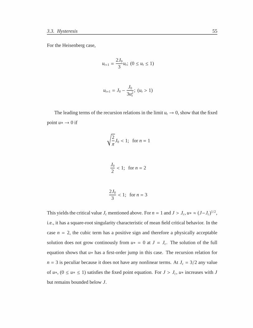
For the Heisenberg case,

ut+1 =2J0

3ut; (0 ≤ ut ≤ 1)

ut+1 = J0 −J0

3u2t

; (ut > 1)

The leading terms of the recursion relations in the limitut → 0, show that the fixed

pointu∗ → 0 if

√

2π

J0 < 1; for n = 1

J0

2< 1; for n = 2

2J0

3< 1; for n = 3

This yields the critical valueJc mentioned above. Forn = 1 andJ > Jc, u∗ ≈ (J−Jc)1/2,

i.e., it has a square-root singularity characteristic of mean field critical behavior. In the

casen = 2, the cubic term has a positive sign and therefore a physically acceptable

solution does not grow continously fromu∗ = 0 at J = Jc. The solution of the full

equation shows thatu∗ has a first-order jump in this case. The recursion relation for

n = 3 is peculiar because it does not have any nonlinear terms. AtJc = 3/2 any value

of u∗, (0 ≤ u∗ ≤ 1) satisfies the fixed point equation. ForJ > Jc, u∗ increases withJ

but remains bounded belowJ.

3.3. Hysteresis 56

3.3.4 Simulations

Figure-3.8 and figure-3.9 show magnetization curves for therandom-field XY and

Heisenberg models, respectively, in a slowly varying cyclic field. The data is obtained

from simulation of the model on a simple-cubic (sc) lattice with nearest-neighbor (nn)

interactions. In order to keep the computer time within reasonable limits, the XY

model is simulated on a lattice of size 1003, and the Heisenberg model on a lattice of

size 503 with periodic boundary conditions. Graphs are presented for various values

of J as indicated in the captions for the figures. For each value ofJ, the applied field

is cycled in small steps between two large values that saturate the magnetization along

negative and positive x axis, respectively. For clarity, the figures depict only a part of

the simulation data in a small range of the applied field wherevariation in magneti-

zation is most pronounced. At each step of the applied field the system is allowed to

relax till it reaches a fixed point. We assume that the system has reached a fixed point

if the projection of each spin along x axis remains invariantwithin an error of 10−5.

The mean-field theory predicts the absence of hysteresis in the XY model if J0 <

1.498. The energy scale in our model is set by the disorder term.Thus the behavior of

the mean-field model atJ0 may be compared with the behavior of the nn model on a sc

lattice at 6J. As an order-of-magnitude estimate, we expect the absence of hysteresis on

a sc lattice if 6J < 1.498 orJ < 0.25 approximately. This is qualitatively in accordance

with the result of simulations shown in Figure-3.8. The magnetization curves forJ =

0.1 show no discernible hysteresis on the scale of the figure. AtJ = 0.2, we find two

isolated hysteresis loops separated by a region of zero hysteresis nearh = 0. This

is qualitatively similar to the prediction of the mean-fieldtheory. With increasing J

the two isolated loops widen, gradually merge with each other, and the overall shape

3.3. Hysteresis 57

of the hysteresis loop evolves as indicated in figure-3.8. For much larger values of

J the hysteresis loop becomes narrower and more vertical. Within numerical errors,

magnetization curves in increasing and decreasing fields approach a step function at

h = 0, and hysteresis appears to vanish forJ ≥ 1. The large J regime marks a qualitative

difference between the prediction of the mean-field theory and the simulations. The

mean-field theory predicts hysteresis but simulations on cubic lattices with nearest-

neighbor interactions show no hysteresis. This discrepancy may be attributed to the use

of infinite range interactions in the mean-field theory. The energy barrier for rotation

of a strategically placed spin may be significantly smaller if its nearest neighbors alone

are taken into account rather than all spins in the system. The dynamics based on

nn interactions initiates a rotation at the least stable site and gradually spreads it on

adjacent sites in the neighborhood. LargeJ simulations take an enormously long time

to reach a fixed point in the neighborhood ofh = 0, but the end result appears to be

simply a reversal of saturation magnetization when the signof h is reversed. In the limit

J→ ∞ the system effectively acts as a single spin having the total magnetization of the

system. Just as an isolated spin in the limitJ = 0 does not show any hysteresis so also

the entire system in the limitJ → ∞. The main difference between the magnetization

curves in the limitsJ → 0 andJ → ∞ lies in their shape, but this is understandable if

we rescale the applied field appropriately with the total magnetization of the system.

Simulations of the Heisenberg model are also in reasonable agreement with the

predictions of the mean-field theory except for large valuesof J. The mean-field the-

ory predicts hysteresis ifJ0 > 3/2. This corresponds toJ > 0.25 approximately.

Simulations do not show any significant hysteresis ifJ ≤ 0.25. Figure-3.9 shows a

magnetization curve forJ = 0.25 that reverses itself when the field is reversed. The

magnetization is linear in the applied field over a wide rangearoundh = 0. This is

3.4. Concluding remarks 58

in qualitative agreement with the prediction of the mean-field theory. Simulations for

J = 0.4 andJ = 0.5 show typical hysteresis loops although the range of applied field

over which perceptible hysteresis is observed is an order ofmagnitude smaller than the

range predicted by the mean-field theory. The main difference between the simulations

and the mean-field theory lies at large values ofJ. Simulations based on smaller steps

and higher accuracy in determining the fixed points suggest that the hysteresis loop

vanishes forJ ≥ 1 and the magnetization has a first-order jump ath = 0.

3.4 Concluding remarks

We have analyzed a simple model to study the effect of quenched disorder on hystere-

sis in magnetic systems of continuous symmetry. The model isobtained by adding

quenched disorder and zero-temperature dynamics to the well established XY and

Heisenberg models of ferromagnetism. The quenched disorder is in the form of ran-

domly oriented fields of unit magnitude. Is this model applicable to experiments? We

have argued that thermal fluctuations are of secondary importance in disorder-driven

hysteresis. Therefore the use of zero-temperature dynamics may not be serious. It has

the virtue of being deterministic and therefore easier to analyze theoretically. A large

number of studies on disordered systems employ zero-temperature dynamics for these

reasons. Randomly oriented crystal fields are also not uncommon in amorphous ma-

terials. These are dipolar or quadrupolar but if the activation barriers are large, may

act like quenched random fields as a spin or domain pointing one way gets hard to

dislodge. Thus the basic ingredients of our model are chosento make a minimal model

for understanding experiments. The parameters of the resulting model are:n com-

ponents of vector spins, exchange interactionJ, and the applied fieldh. Effectively,

3.4. Concluding remarks 59

there are just two parameters ; integern and realJ. This is because the middle term in

Hamiltonian (3.1) does not have a tunable value, and the fieldh is cycled between−∞

and∞ . A two parameter model may not capture details of hysteresisin various ma-

terials but it provides a caricature of experimental observations. The variety of shapes

of hysteresis loops are particularly striking for the XY model (n = 2). As J is varied,

we get familiar as well as rather unusual shapes of loops. Theunusual shapes have

been noted earlier in magnetic and other materials. These are known as wasp-waisted

[24] or double-flag shaped loops [127].These shapes have a kind of weak universality

in the sense that they are seen in the mean-field theory, simulations on three dimen-

sional lattices, and experiments in diverse systems. Similar shapes are also seen in the

random-field Blume-Emery-Griffiths model and other models of plastic depinning of

driven disordered systems.

Soft continuous spins with Gaussian random fields have been used earlier to study

critical hysteresis in 6−ǫ dimensions in the renormalization-group theory. Where does

our mean-field calculation sit in this context? We note that our mean-field results do

not match the renormalization-group results in any limit. There are two possible rea-

sons for this. First, we have used a different distribution of random fields than the

one used in 6− ǫ expansion. The form of random-field distribution appears tobe im-

portant in determining critical hysteresis. Second, we do not have the benefit of an

appropriate renormalization-group study of our variant ofthe model, nor do we know

the upper critical dimension of our model precisely. Beforethe renormalization-group

theory, mean-field theory was viewed as an approximate but self consistent theory of

critical behavior in three dimensions because it neglectedfluctuations. This variant

of mean-field theory was based on infinitely weak but long ranged interactions in the

3.4. Concluding remarks 60

system. It represented the effect of the entire system on an individual spin by an ef-

fective field while keeping the energy of the system extensive. The renormalization

group has given another connotation to mean-field theory. Inits framework, the mean-

field theory becomes a reduced theory based on a quadratic action that is exact at and

above an upper critical dimension where fluctuations are negligible. The upper critical

dimension for pure nondisordered magnetic systems is four,and in this case the two

variants of the mean-field theory predict the same critical behavior. This is understand-

able because the effective field is proportional to the order parameter and the effective

action is therefore quadratic. The upper critical dimension for a disordered spin model

with a Gaussian random field is six [126]. In this case also, an explicit calculation

for the random-field Ising model with Gaussian field shows that the two variants of

mean-field theory yield the same critical behavior. However, when the randomness is

of the form of randomly oriented unit vectors, we have analyzed only one variant of

mean-field theory that is based on infinitely weak but long-range forces. It predicts

strikingly different critical behavior in XY and Heisenberg models, respectively. The

casen = 2 has a first-order transition , andn = 3 an unusual transition as discussed

before. A somewhat similar case of first as well as second-order depinning transition

in the mean-field theory occurs in a viscoelasic model of driven disordered systems

[128, 129] Thus we have a number of model-specific results. Evidently more work is

required to make any general connection between the random-field distribution and the

nature of criticality in the model, and to connect a conventional mean-field theory to a

limiting form of renormalization-group theory above an upper critical dimension.

The new framework for understanding critical behavior alsouses the idea of a lower

critical dimension. Below the lower critical dimension thefluctuations are so great that

the system does not order at all and therefore there is no question of a phase transition.

3.4. Concluding remarks 61

The lower critical dimension for an equilibrium transitionin an n-component spin sys-

tem in a Gaussian random field is 2 forn = 1, and 4 forn ≥ 2. To our knowledge, the

lower critical dimension for the case of randomly oriented unit vectors is not known.

However, we mention a few issues that may bear on experimentsin three dimensions ir-

respective of the form of randomness characterizing the system. It has been argued that

critical hysteresis in a Gaussian random-field Ising model is in the same universality

class as the corresponding equilibrium critical point [68, 69, 70, 78]. There is a reason-

able experimental evidence for this [68, 69, 70]. In the case of Gaussian random-field

XY and Heisenberg models, the lower critical dimension liesabove three. Does it nec-

essarily mean the absence of critical hysteresis in these models in three dimensions?

The situation is not entirely convincing either theoretically or experimentally. The ar-

gument for a lower critical dimension is based on spontaneous symmetry breaking in

the absence of an applied field. If the critical point on the hysteresis loop were to occur

at a nonzero value of magnetization or the applied field then aunique direction is al-

ready chosen by the corresponding magnetization or the applied field. In this case we

may observe critical hysteresis in three dimensions with critical exponents appropriate

for the Gaussian random-field Ising model. Much of critical hysteresis seen in experi-

ments may belong to this case but there is discrepancy between some experiments and

theory [79]. It may be that quenched disorder in experimental systems is not charac-

terized adequately by Gaussian random fields or randomly oriented unit vectors. The

presence of demagnetizing fields and dipolar forces in materials used for experiments

are likely to change the simple theoretical picture based onon-site random-field disor-

der. This applies equally to mean-field theory and the renormalization-group approach

based on expansions around a quadratic action.

In the absence of exact solutions in three dimensions, simulations of models may

3.4. Concluding remarks 62

be more relevant to experiments. Our simulations produce rather smooth hysteresis

loops for small and moderate values of J suggesting the absence of jumps in the mag-

netization. Phase transitions in complex systems are difficult to decide on the basis of

numerical work alone, and therefore we have focused on the shape of hysteresis loops.

The shapes are not universal but this does not diminish theirimportance in the appli-

cation of magnetic materials. The relationship between theshape of hysteresis loops

and the defect mediated process of magnetization reversal is also interesting. This has

been studied at zero temperature numerically in a two-dimensional XY model with

weak random anisotropy [118]. We hope future studies on these lines will clarify the

relationship of the hysteresis loops to the underlying energy landscape as well as the

patterns of spin configurations such as vortex loops in threedimensional XY model.

α iiθ

J0m(t) + h

(t+1)

F 3.1: A geometrical representation of the dynamics of randomfield XY model.The figure shows a vector relationship between the updated spin ~Si(t+ 1), the random

field~hi , and the mean fieldJ0m(t) + h at sitei.

3.4. Concluding remarks 63

m (

h=0)

J0

0

0.1

0.2

0.3

0.4

0.5

0.6

0.7

0.8

0.9

1

0 0.5 1 1.5 2 2.5 3

F 3.2: (Color online) Fixed points of the random fieldXY model in zero appliedfield and different values of exchange interactionJ0. In this figure, The blue curvecorresponds to increasingJ0; at each value ofJ0, the fixed point configuration of theprevious lower value ofJ0 is used as an input into the equations of dynamics. ForincreasingJ0, the magnetization of the fixed point is zero in the range 0≤ J0 ≤ 2.At J0 = 2, it jumps tom ≈ .92, and follows the blue curve asJ0 is further increased.The return path in decreasingJ0 is identical with the blue curve up toJ0 ≥ 2, but itcontinues along the green curve up toJ0 ≈ 1.49 at which point it jumps fromm≈ .74to m = 0 and remains zero for 0≤ J0 ≤ 1.49. The red curve shows a set of unstable

fixed points.

3.4. Concluding remarks 64

f(u)

u

0

0.2

0.4

0.6

0.8

1

0 0.5 1 1.5 2

F 3.3: (Color online) A plot off (u) vs u; andu/J0 vs u for J0 = 1.489, andJ0 = 2. The figure shows why the mean field dynamics of the random field XY model

has multiple fixed points in the range 1.489≤ J0 ≤ 2

3.4. Concluding remarks 65

m(h

)

h

−1

−0.8

−0.6

−0.4

−0.2

0

0.2

0.4

0.6

0.8

1

−1.5 −1 −0.5 0 0.5 1 1.5

F 3.4: (Color online) Hysteresis in the random fieldXY model in the mean fieldapproximation. The figure shows magnetization in the systemas the applied fieldhis cycled along thex-axis for three representative values ofJ0; J0 = 2 (blue), J0 =

1.25 (green), andJ0 = .25 (red). The random field has a fixed magnitude equal tounity. The hysteresis loop forJ0 = 2 has a familiar shape butJ0 = 1.25 shows ratherunusual hysteresis in two small windows of applied field situated ath ≈ −.2, andh ≈ .2 respectively but no hysteresis outside these windows. In particular, there is nohysteresis at or near zero applied field. ForJ0 = .25, there is no discernible hysteresis

in any region of the applied field on the scale of the above figure.

3.4. Concluding remarks 66

f(u)

u

0

0.2

0.4

0.6

0.8

1

0 0.2 0.4 0.6 0.8 1 1.2 1.4

F 3.5: (Color online) A plot of f (u) vs u and (u − h)/J0 for J0=1.25 andh=0.1,0.2 and 0.3. Lines corresponding toh = .1 andh = .3 cut f (u) at a single point butthe line corresponding toh = .2 cuts f (u) at three points. This accounts for two small

hysteresis loops seen in figure-3.4 ath = ±.2 andJ = 1.25.

3.4. Concluding remarks 67

g(u)

u

−1

−0.5

0

0.5

1

−3 −2 −1 0 1 2 3

F 3.6: (Color online) A Graph ofg(u) vs u for −3 ≤ u ≤ 3 superimposed on aline u/J0 for J0 = 3/2. The figure shows thatg(u) coincides with the line 2u/3 in therange−1 ≤ u ≤ 1. If J0 < 3/2, the lineu/J0 cutsg(u) only atu = 0. If J0 > 3/2 the

line u/J0 cutsg(u) at three points including the pointu = 0.

3.4. Concluding remarks 68

m(h

)

h

−1

−0.8

−0.6

−0.4

−0.2

0

0.2

0.4

0.6

0.8

1

−1 −0.5 0 0.5 1

F 3.7: (Color online) Hysteresis loops in the random field Heisenberg model inthe mean-field approximation. The figure shows magnetization curves forJ0 = 2 (red)andJ0 = 1.75 (green). There is no hysteresis ifJ0 ≤ 1.5. Magnetization curves areshown forJ0 = 1.5 (blue) andJ0 = 1 (pink); magnetization may show a discontinuity

at h = 0 if J0 = 1.5.

3.4. Concluding remarks 69

m(h

)

h

−1

−0.8

−0.6

−0.4

−0.2

0

0.2

0.4

0.6

0.8

1

−1 −0.5 0 0.5 1

F 3.8: (Color online) Magnetization in the random fieldXY model on a 1003

simple cubic lattice under a cyclic field. The figure shows different values ofJ: J = .1(red),.2 (green),.25 (blue),.4 (pink), and 1 (light blue).

m(h

)

h

−1

−0.5

0

0.5

1

−0.2 −0.15 −0.1 −0.05 0 0.05 0.1 0.15 0.2

F 3.9: (Color online) Magnetization in the random field Heisenberg model on a503 simple cubic lattice under a cyclic field. The figure shows different values ofJ:

J = .25 (red),.4 (green),.5 (blue), and.9 (pink).