CHAPTER 3: DATA AND RESULTS

CHAPTER 3:

DATA AND RESULTS

75

3.1 Introduction

This chapter documents how the data were collected and employed. It presents the

results derived from the theoretical framework presented in the previous chapter and

provides an analysis of the results.

3.2 Data collection

Two types of data were collected for the study. International organization

databases and literature provided general economic information and aggregate economic

data. These secondary data are discussed in sub-section 3.2.1. Interviews in Senegal and

materials provided in Senegal provided more specific data, particularly on La Fleur 11.

These primary data are presented in sub-section 3.2.2. Sub-section 3.2.3 explains how

secondary and primary data were used to develop parameters for the analysis. Appendix

B contains all the data employed in the analysis.

3.2.1 Data collected from secondary sources

Economic and financial statistics including growth rates of per capita income,

interest rates, and exchange rates were obtained from the International Monetary Fund

(IMF). Also, the IMF provided information about researchers salaries to estimate La

Fleur 11 research costs since information on research costs was difficult to obtain. These

statistics are presented in tables 3.1 through 3.4.

Table 3.1 presents the average annual growth of per capita Gross National

Product (GNP) for the decades 1976-86, 1987-97 and for the period 1998-2002. The

average annual growth of per capita GNP was negative in the two first periods, but

positive in the last period.

76

Table 3.1: Average annual growth of per capita GNP (Gross National Product) in Senegal 1976-1986 1987-1997 1998-2002 GNP per capita -0.011 -0.004 0.034

Source: IMF, 1998.

Table 3.2 presents the interest rates applied in the money market in Senegal in the

period 1993 through 1998. It decreased during the entire period. In 1993 and in the first

half of 1994 it was within the range 0.07-0.09. In 1995-97, it was between 0.05 and 0.06.

In 1998, it was between 0.045 and 0.05. The IMF provides another interest rate, 0.0625,

which was applied by the Central Bank of Senegal to all loans after August 31st 1998

(IMF, 2000).

Table 3.2: Interest rates applied in the money market in Senegal Periods Interest rate

1993 October

November December

1994 January March June

September December

1995 March June

September December

1996 January

February March April May June July

August September

October November December

1997 January

February March April

0.0935 0.085 0.0751

0.0794 0.0925 0.0885 0.0567 0.055

0.055 0.055 0.055 0.0578

0.0551 0.055 0.055 0.0548 0.0521 0.0537 0.0541 0.0525 0.0525 0.0525 0.052 0.0505

0.0504 0.0511 0.05 0.05

77

May June July

August September

October November December

1998 January

February March April May June July

August September

0.05 0.0502 0.0502 0.0502 0.0502 0.0502 0.0502 0.0496

0.0451 0.0450 0.0453 0.0456 0.0478 0.0495 0.0495 0.0496 0.0496

Source: IMF, 2000. Table 3.3 presents the exchange rates of CFA Francs for US Dollars. The

exchange rate has increased since 1995 with an average annual growth rate of 4.6

percent.

Table 3.3: Exchange rate CFA Franc-US Dollar Period average 1994 1995 1996 1997 1998* 1999 CFA Franc/U.S. $ 555.20 499.15 511.55 583.50 595.56 615.70

*: Jan-Oct Source: IMF, 2000 and CIA, 2001.

Table 3.4 presents public salaries. Only the maximum and the minimum monthly

salaries paid to some employees in Senegal are available. These salaries didn’t vary much

during the period 1985-1998. The average maximum salary is 237,414 CFA Francs per

month. The average minimum salary is 40,863 CFA Francs per month. According to a La

Fleur 11 breeder, the maximum salaries represent a good approximation of the salaries

paid to the scientists who developed La Fleur 11 (Ndoye, April 24th 2001).

Table 3.4: Maximum and minimum salaries for selected civil servants in Senegal CFA Francs/month Jan. 1985 July 1989 Sept. 1993 Jan. 1994 After Apr. 1994 Minimum salary 36,462 40,482 34,409 40,482 52,482 Maximum salary 238,165 242,184 205,855 242,184 258,684

Source: IMF, 2000.

78

Additional information about researchers salaries was provided by ISRA. Ndoye

(April 24th, 2001) provided information about the salaries paid to the assistants who

participated to the development of La Fleur 11. Although he mentioned that the assistants

received monthly salaries between 70,000 and 110,000 CFA Francs, he suggested that a

good average of their monthly salaries is 75,000 CFA Francs.

The Food and Agriculture Organization of the United Nations (FAO) provided

data on production quantities and export and import quantities and values of peanut

products in Senegal as shown in table 3.5. Production and exports vary greatly from year

to year. The production of unshelled peanuts and peanut seeds are correlated. The

production and exports of oil and cakes are correlated as well. Besides unshelled peanuts,

seeds and cakes are the two most important peanut products because they come from two

industries, oil processing and confectionery. For the period considered, there are no

imports of unshelled peanuts, peanut seeds, peanut oil and peanut cakes and unshelled

peanuts and peanut seeds are not exported.

Table 3.5: Total production, imports and exports of peanut products in Senegal Tons 1994 1995 1996 1997

Production Unshelled peanuts ( for oil industry) Seeds (oil and confectionery industries) Oil Cakes (oil and confectionery industries)

678,040 102,000 98,191

122,739

790,617 120,000 111,259 139,074

588,181 88,000

167,277 209,096

505,894 76,000

118,243 147,804

Imports - - - Exports Unshelled peanuts (for oil industry) Seeds (oil and confectionery industries) Oil - Quantity (tons) - Value ($1,000) Cakes (oil and confectionery industries) - Quantity (tons) - Value ($1,000)

- -

73,471 73,676

83,768 12,354

- -

54,518 53,814

37,163 5,026

- -

99,000 38,622

88,300 6,322

- -

43,030 40,000

45,844 2,500

Source: FAO, 1999.

79

Estimates of peanut supply and demand elasticities were found in the literature.

Economic studies provided four different estimates of the supply elasticity for unshelled

peanuts: 0.77 (Akobundu, 1998), 0.4889 (Lopez and Hathie, 1998), 0.433 (Gaye, 1998 b)

and 0.16 (Sullivan et al, 1992). The first estimate is used in the analysis on the basis of

the following argument. Alston et al (1995) explain that the choice of a linear supply

curve generates an over-estimation of the supply shift and research benefits when supply

is inelastic. This over-estimation can be corrected by choosing the highest supply

elasticity estimate such that the gross cost reduction per unit of output ∆Y/εY is adjusted

downward and hence the supply shift and research benefits are lowered as well. Only one

estimate of demand elasticity for unshelled peanuts was found in the literature: -0.18

(Sullivan et al, 1992). For peanut oil, only one estimate of supply elasticity and one

estimate of demand elasticity were found in the literature, 0.3 and –0.2 respectively

(Sullivan et al, 1992)9. In the absence of estimates of supply and demand elasticities for

peanut cakes, it is assumed that the oil elasticities are also valid for cakes.

Previous studies on the peanut sector in Senegal provided information on farm

household consumption and the informal and formal peanut markets in Senegal. This

information is presented in table 3.6.

Table 3.6: Relative importance of the main commodities of the Senegalese peanut market

PEANUT SUPPLY 100% OFFICIAL MARKET 65% FARM 24% UNOFFICIAL MARKET 11%

NOVASEN Seeds

Peanut meal Cakes

SONACOS Seeds

Peanut oil Cakes

Seeds 9%

Consumption 3% Gifts … 12%

Unshelled peanuts 10%

Shelled peanuts Oil and paste

Source: Gaye (1997, 1998 a).

9 The elasticities found in Sullivan et al (1992) are for oil seeds other than soy seeds and oils other than soy oil.

80

Farm household consumption is considered as a whole with 24 percent of the total

peanut supply; no differential is made between the different farm household utilizations

of supply. In the official market, only SONACOS production is considered in the analysis

because La Fleur 11 is an oil seed and hence is not used in the confectionery industry.

Therefore, the 65 percent are assumed to include SONACOS purchases only. According

to Gaye (February 22nd, 2001), from one ton of unshelled peanuts purchased from

farmers SONACOS produces 0.35 tons of oil and 0.35 tons of cakes. In the unofficial

market, only unshelled peanuts are considered in the analysis with 10 percent of the total

peanut supply because they constitute the greatest part of this market. Prices of unshelled

peanuts sold on the unofficial market are presented in table 3.7. They are given for three

periods of each year. The second period coincides with the opening of the official market.

Prices vary between 125 and 160 CFA Francs/kg.

Table 3.7: Unshelled peanut prices on the unofficial market in Senegal 1995-96 1996-97

CFA Francs/kg First period Second period Third period First period Second period Third period Unshelled peanuts 125.40 128.00 129.50 130.30 139.70 160.40

Source: Gaye (1997, 1998 a).

3.2.2 Data collected in Senegal

The rest of the data used in the analysis was collected in Senegal. General

information and data about the peanut sector were found at the Ministry of Finance and

the Ministry of Agriculture. The Ministry of Finance provided peanut prices and

subsidies since the application of the new peanut pricing policy in 1996 as shown in table

3.8. There are two domestic official prices for unshelled peanuts: the producer base price,

which is set according to the peanut pricing policy and the consumer price which is the

actual price farmers receive from sales to SONACOS. In 1996-97, the consumer price

81

was higher than the producer base price. In the other years, the producer base price was

higher causing the government to pay a subsidy to the farmers.

Table 3.8: Unshelled peanut official prices in Senegal CFA Francs/kg 1996-97 1997-98 1998-99 1999-00

Producer base price 131.00 150.00 160.00 145.00 Consumer price 183.00 137.656 114.00 142.00

Source: Senegal, Republic of, Ministère de l’Economie, des Finances et du Plan, 2000 a.

The world prices for oil and cakes were found in Oil World Annual. As shown in

table 3.9, in the period 1994-00 the peanut oil world price was around 900 U.S. Dollars

per ton and the peanut cake world price was around 160 U.S. Dollars per ton.

Table 3.9: Peanut world prices Period average

US$/ton 1994 1995 1996 1997 1998 1999 2000

Peanut oil 1,023 991 897 1,009 917 788 740 Peanut cakes 168 169 213 221 116 102 130

Source: Senegal, Republic of, Ministère de l’Economie, des Finances et du Plan, 2000 a.

The Statistical Service of the Ministry of Finance provided statistics on the

growth rate of population, 0.027 for the entire country for the period 1988-98 (Senegal,

Republic of, Direction de la Prévision et de la Statistique, 1999)10. The Ministry of

finance also provided regulatory information about peanut policies (Senegal, Republic of,

Direction de la Prévision et de la Statistique, 1999). This information was presented in

chapter 1.

The Statistical Service of the Ministry of Agriculture provided statistics on peanut

production in Senegal for the last fifteen years and for each political district. Table 3.10

reports the quantities produced for the entire country for the period 1996-99. This period

is chosen because producer base prices are only available for the years 1996 through

10 The projection of the population growth rate in Senegal for the period 1997-2015 is 0.025 (UNDP, 1999). It is not very different from the Senegalese population growth rate used in the analysis, 0.027.

82

2000. Only the portion of the production that is used in the oil processing industry is

presented. The output of year 1999-2000 is the highest because of favorable rainfall.

Table 3.10: Production quantities of unshelled peanuts (oil seeds) in Senegal 1996-97 1997-98 1998-99 1999-00

Tons 588,181 505,894 540,773 764,077 Source: Senegal, Republic of, Ministry of Agriculture, 2000.

ENEA (Ecole Nationale d’Economie Appliquée), ISRA, Sonagraines and UNIS

provided specific information and data on La Fleur 11. ENEA provided a study with

farm-level yields for the old variety 55-437, 396 kg/ha, and the new variety La Fleur 11,

515 kg/ha (Bravo-Ureta et al, 1998). ISRA provided the yield increase of La Fleur 11, 30

percent in comparison to the variety 55-437’s yield (Ndoye; July 19th, 2000), information

on the number of researchers who worked on La Fleur 11, and the number of years where

they worked on La Fleur 11 as indicated in table 3.11. During the research and

development lag, two breeders and two agronomists worked on La Fleur 11. In total five

assistants worked with the scientists on La Fleur 11. These assistants had other duties

besides the development of la Fleur 11.

Table 3.11: Number of researchers who participated in the development of La Fleur 11

Researchers by category Years of participation Breeder 1 Breeder 2

Agronomist 1 Agronomist 2

Assistant 1 Assistant 2 Assistant 3 Assistant 4 Assistant 5

7 5 4 2 12 10 5 4 4

Source: Ndoye; February 22nd, 2001.

Sonagraines provided information about agricultural practices of peanut farmers

using La Fleur 11 seeds (Boye, 2000). This information was presented in chapter 1.

83

UNIS provided some data and information for the evaluation of the change in

input costs due to the adoption of La Fleur 11. The change in variable costs mainly

corresponds to a change in seed cost. Few farmers use more fertilizer and/or pesticides

when adopting La Fleur 11 and information on their use is not available. Table 3.12

presents the quantities and prices of seeds used for the old variety 55-437 and the new

variety La Fleur 11.

Table 3.12: Seed quantities and prices for peanut varieties 55-437 and La Fleur 11 1998-99 1999-00 55-437 Quantity (kg/ha)

Price (CFA F/kg) 120 205

120 190

La Fleur 11 Quantity (kg/ha) Price (CFA F/kg)

150 250

150 225

Source: Ndoye D., 2000.

3.2.3 Use and configuration of data for the analysis

La Fleur 11 started being marketed in 1997, which corresponds to the beginning

of the second lag of the adoption profile where the adoption rate started increasing and

the supply curve started shifting (see below). Therefore, it would have been appropriate

to choose the period 1994-96 for the approximation of the initial equilibrium. However,

data on the producer base price are only available for the period 1996-2000.

Consequently, all the prices and quantities used in the analysis correspond to this period

of time. Data on prices and quantities are averaged. The price is calculated in CFA Francs

per kilogram. When prices are only available in U.S. Dollars, the average exchange rate

for CFA Francs for the corresponding years is used to convert them. The quantities are in

kilograms. From the total supply of unshelled peanuts at the farm level (provided by the

Ministry of Agriculture), the supply of each peanut commodity is determined as a

fraction of the total supply of unshelled peanuts. From the above information tables 3.13

and 3.14 are derived. Table 3.13 contains the average prices of the different peanut

84

products considered in the analysis and the average exchange rate. Table 3.14 contains

the average supply of unshelled peanuts and for each peanut product its proportion in the

entire supply of unshelled peanuts. For the evaluation of the farm sales of unshelled

peanuts on the official market, the producer base price 146.50 CFA Francs/kg applies to

the entire production of unshelled peanuts, 599,731 tons. When other peanut commodities

are considered, their corresponding price is used and their supply is calculated as a

portion of the entire supply of unshelled peanuts.

Table 3.13: Average peanut product prices and exchange rate Average Reference Producer base price of unshelled peanuts 146.50 CFA Francs/kg Table 3.8 Consumer price of unshelled peanuts 144 CFA Francs/kg Table 3.8 Unofficial price of unshelled peanuts 135.55 CFA Francs/kg Table 3.7 Price of seeds for variety 55-437 197.50 CFA Francs/kg Table 3.12 Price of seeds for variety La Fleur 11 237.50 CFA Francs/kg Table 3.12 World price of peanut oil 909 US$/ton* Table 3.9 World price of peanut cakes 160 US$/ton* Table 3.9 Exchange rate 560.11 CFA Francs/US$ Table 3.3

* The prices in US Dollars are converted to CFA Francs using the average exchange rate. Table 3.14: Average quantity supplied of unshelled peanuts and proportion of each peanut commodity in the total supply of unshelled peanuts in Senegal

Average Reference Production of unshelled peanuts (for oil processing) 599,731 tons Table 3.10 Ratio of on farm consumption of unshelled peanuts 0.24 Table 3.6 Ratio of farm sales of unshelled peanuts on the unofficial market 0.10 Table 3.6 Ratio of total farm sales of unshelled peanuts to SONACOS 0.65 Table 3.6 Ratio of farm sales of peanut seeds to SONACOS 0.15* Table 3.5 Ratio of farm sales of unshelled peanuts for oil processing by SONACOS 0.50** Derived Ratio of SONACOS production of oil in purchases of unshelled peanuts 0.35 (Gaye, 2001) Ratio of SONACOS production of cakes in purchases of unshelled peanuts

0.35 (Gaye, 2001)

Ratio of SONACOS sales of peanut oil in total supply of unshelled peanuts

0.175*** derived

Ratio of SONACOS sales of peanut cakes in total supply of unshelled peanuts

0.175*** derived

Proportion of peanut oil exports in peanut oil supply 0.54**** Table 3.5 Proportion of peanut cake exports in peanut cake supply 0.41**** Table 3.5

* Calculated by dividing the average seed production by the average production of unshelled peanuts ** Calculated by subtracting the seed ratio to SONACOS total ratio (0.65-0.15) *** Calculated by multiplying SONACOS ratio of unshelled peanuts purchased and the ratio of oil and cake production (0.5*0.35) **** Calculated by dividing the average oil and cake exports respectively by the average production of unshelled peanuts

85

The growth rate of demand in Senegal is calculated by summing the growth rate

of population and the product of income elasticity of demand and the growth rate of per

capita income. The growth rate of population is given for the period 1988-1998, 2.7

percent per year. The growth rate of per capita income is an average calculated from table

3.2, 0.63 percent per year11. The income elasticity is estimated using the homogeneity

condition, which states that the sum of the own-price demand elasticity, the cross-price

demand elasticities and the income elasticity equals zero. Alston et al (1995) estimate the

income elasticity by assuming that the sum of cross price elasticities is a small number

when no information on cross-price elasticities is available. To avoid any arbitrary

estimation of that number, the sum of cross price elasticities is assumed to be zero, which

is an empirically accepted approximation. Thus the income elasticity equals the negative

of the own-price demand elasticity. These results are shown in table 3.15. As a result of a

very small income growth, the growth rate of demand, 2.8 percent per year is very close

to the growth rate of population.

Table 3.15: Data used for the calculation of the demand growth rate in Senegal Ratios Reference Growth rate of population per year 0.027 Senegal, Republic of, Direction de la

Prévision et de la Statistique, 1999 Growth rate of per capita income per year 0.0063 Table 3.1 Income elasticity per year 0.18 Derived Growth rate of demand per year 0.028 Derived

For the calculation of the supply shift K, two approximations are made. The first

approximation is about fixed costs, which are assumed to remain unchanged between the

without-research and with-research situations. The second approximation is about the

11 Maybe only the period 1987-97 should have been considered for the estimation of the growth rate of per capita income, but a negative value might not reflect the actual growth rate in the next decades. A better estimate of this rate may have been to compute the average growth rate by weighting it by the number of years in each period.

86

depreciation rate, which is not taken into consideration (see below). The estimation of the

research-induced supply shift requires several steps:

- The comparative yield increase between 55-437 and La Fleur 11 is 30 percent.

This figure represents the experimental gain in yield and the farm-level yield

increase as well (515-396/396).

- The yield increase 0.30, which corresponds to a horizontal shift of the supply

curve, is divided by the supply elasticity 0.77 in order to obtain the gross cost

reduction per unit of output: 0.39, which corresponds to a vertical shift of the

supply curve.

- In order to transform the gross cost reduction per unit of output into a net cost

reduction per unit of output, the research-induced change in total cost per unit

of output has to be subtracted from the gross cost reduction per unit of output.

The estimation of the research-induced additional total cost per unit of output

is based on several calculations involving the research-induced change in seed

cost.

- The change in seed cost is calculated using La Fleur 11’s and 55-437’s seed

quantities and prices given in table 3.12: (150*237.50)-(120*197.50) = 11,925

CFA Francs per hectare.

- This amount represents an increase in seed cost equal to 0.5 relative to the

without-research seed cost (11,925/23,700). The without-research seed cost is

calculated on the basis of the seed cost for variety 55-437: 120*197.50 =

23,700 CFA Francs per hectare.

87

- The without-research seed cost, 23,700 CFA Francs per hectare, represents a

fraction of the without-research total cost. The latter is approximated using

total revenues12. Total revenues are calculated on the basis of the initial

equilibrium output price, 146.50 CFA Francs and yield, 396 kg/ha,

146.50*396 = 58,014 CFA Francs per hectare. Therefore, the ratio seed cost

over total cost is 23,700/58,014 = 0.4113.

- Consequently, the proportionate additional total cost per hectare is 0.50*0.41

= 0.20.

- The proportionate change in yield is used in order to transform the

proportionate additional cost per hectare into a proportionate additional cost

per unit of output, 0.20/(1+0.30) = 0.15.

- The net cost reduction per unit of output, 0.24 is calculated by subtracting the

proportionate additional cost per unit of output, 0.15 from the gross cost

reduction per unit of output, 0.39.

- The supply shift K is obtained by multiplying the net cost reduction per unit

of output by the probability of research success, the annual adoption rate and

the initial equilibrium price. Regarding the probability of research success, it

is assumed that the yield increase is successfully achieved (100 percent) based

on the information given in chapter 1. For the commodities produced on farm,

the supply shift is calculated on the basis of the corresponding initial

equilibrium price (producer base price for unshelled peanuts sold on the

12 In economic theory, the supply curve corresponds to marginal costs. Thus, the output price can be used as an approximation of per unit of output production costs. 13 In this case, only the producer base price is used. Table 3.18 presents the calculation of the supply shift with the unofficial market price also.

88

official market and unofficial market price for unshelled peanuts consumed on

farm or sold on the unofficial market). For the commodities sold by

SONACOS (peanut oil and cakes) the supply shift is assumed to be the same

as for the unshelled peanuts sold to SONACOS.

These calculations are summarized in table 3.16.

Table 3.16: Data used for the calculation of the peanut supply shift in Senegal Data Reference Proportionate yield increase per hectare ∆Y/Y 0.30 Ndoye, July 19th 2000 and

Bravo-Ureta et al, 1998 Gross proportionate cost reduction per unit of output ∆Y/Yε

0.39 0.30/0.77

Additional seed cost per hectare 11,925 CFA Francs/ha (150*237.50)-(120*197.50) Proportionate additional seed cost per hectare 0.50 11,925/(120*197.50) Fraction of seed costs in total costs (revenues): - using producer base price - using unofficial market price

0.41 0.42

(120*197.50)/(396*146.50)

(120*197.50)/(396*141) Proportionate additional total cost per hectare ∆C/C: - using producer base price - using unofficial market price

0.20 0.21

0.50*0.41 0.50*0.42

Proportionate additional total cost per unit of output ∆C/C(1+∆Y/Y): - using producer base price - using unofficial market price

0.15 0.16

0.20/(1+0.30) 0.21/(1+0.30)

Net proportionate cost reduction per unit of output ∆Y/Yε - ∆C/C(1+∆Y/Y): - using producer base price - using unofficial market price

0.24 0.23

0.39-0.15 0.39-0.16

Probability of research success p 1 Assumed Adoption rate See table 3.18 Ndoye, February 22nd 2001 Initial equilibrium price 146.50 CFA Francs/kg

141 CFA Francs/kg Table 3.13

Post demand shift equilibrium price

In the absence of information about the adoption lags and rates, the maximum rate

of adoption and the length of the second lag are approximated on the basis of the

available information. Since research on La Fleur 11 started in 1985 and La Fleur 11 was

marketed in 1997, the duration of the research and development lag is 12 years (1985-

1996). The second lag is the current lag; the adoption rate is increasing. According to a

La Fleur 11 breeder, the second lag will be very long and the adoption will be constrained

by exogenous factors such as seed demand and supply (Ndoye, February 22nd 2001).

89

Accordingly, the analysis will be based on different approximations of the second

adoption lag (a short lag and a long lag) and of the maximum adoption rate (a low rate

and a medium rate). The lengths considered are 10 and 20 years. A lag longer than 20

years seems to be unlikely because another new variety will probably be developed by

then. The maximum adoption rates considered are 15 and 25 percent. A higher adoption

rate is not employed for several reasons. La Fleur 11 is currently preferred to 55-437

because it produces larger peanuts and can be sold before the regular harvest period as

peanut meal at a high price in the informal market for 300-400 CFA Francs/kg (Boye,

2000). However, because La Fleur 11 is less resistant than 55-437 to aflatoxins, a phyto-

sanitary problem may appear and impede the early marketing of peanut meal reducing

farmers’ demand for La Fleur 11. Adoption of La Fleur 11 may also be limited due to the

potential risk of cake contamination by aflatoxins though this problem doesn’t exist with

oil because aflatoxins are eliminated during the oil refinement process. Also, La Fleur 11

is not suitable for all environments; it was developed for the central area of the peanut

basin and to date has been adopted most in that area. In addition, SONACOS currently

ensures the supply of high quality seeds. When La Fleur 11 seeds begin to be marketed in

the informal market, their quality will probably fall and reduce the farmers’ willingness

to acquire this seed.

Assuming that the adoption profile is linear, the increasing curve of the adoption

profile takes the form: rate = intercept + slope*year. In the first (pessimistic) scenario

where the second lag is 20 years and the maximum adoption rate is 0.15, the intercept and

the slope can be derived from points (12 years;0 adoption rate) and (32 years;0.15

adoption rate). That is from the resulting system of equations, 0 = intercept + slope*12

90

and 0.15 = intercept + slope*32, the intercept and the slope can be simultaneously solved

for: intercept = -0.09 and slope = 0.0075. Thus, the increasing adoption curve is: rate = -

0.09 + 0.0075*year. Similarly, the following function is derived for the second

(optimistic) scenario where the second lag is 10 years and the maximum adoption rate is

0.25: rate = -0.3 + 0.025*year.

Assuming that depreciation doesn’t affect the net present value of the benefits

very much because early years weigh more heavily than later years in the calculation of

the NPV (Alston et al, 1995), table 3.17 is derived to describe the adoption profile in both

scenarios. The first scenario is likely to be the most probable given the information in

hand. It has lower adoption rates than the second scenario.

Table 3.17: Adoption rates in scenarios 1 and 2 Years Scenario 1 (20 years,

15 percentage adoption) Scenario 2 (10 years,

25 percentage adoption) 1≤years≤12 0 0

13 0.0075 0.025 14 0.015 0.05 15 0.0225 0.075 16 0.03 0.1 17 0.0375 0.125 18 0.045 0.15 19 0.0525 0.175 20 0.06 0.2 21 0.0675 0.225 22 0.075 0.25 23 0.0825 0.25 24 0.09 0.25 25 0.0975 0.25 26 0.105 0.25 27 0.1125 0.25 28 0.12 0.25 29 0.1275 0.25 30 0.135 0.25 31 0.1425 0.25

Years≥32 0.15 0.25

Research costs are estimated on the basis of the salaries paid to one or two

scientists (a breeder and an agronomist) and two to four assistants from 1985 to 1996. In

91

the absence of information about the salaries paid to the scientists, it is assumed that the

scientists receive the maximum salary provided by the IMF (table 3.5). Although the

assistants receive a higher salary (on average 75,000 CFA Francs per month) than the

minimum salary provided by the IMF, the minimum salary is used because the assistants

were also involved in other activities than research on La Fleur 11. As shown in table

3.18, the total amount of salaries is calculated for each year in CFA Francs. The annual

researcher salaries are between 4 and 7 million CFA Francs during the research and

development lag. When augmented by 20 percent to account for other costs than salaries

(operating costs), the annual research costs obtained vary between 5 and 9 million CFA

Francs.

Table 3.18: Research costs for the development of La Fleur 11 a) Elements for the approximation of the cost of research salaries

Scientists Assistants Years number Monthly salaries

(FCFA) Number Monthly salaries

(FCFA) 1985 1 238,165 3 36,462 1986 1 238,165 3 36,462 1987 1 238,165 3 36,462 1988 1 238,165 3 36,462

Jan-Jun 1989 1 238,165 3 36,462 Jul-Dec 1989 1 242,184 3 40,482

1990 1 242,184 3 40,482 1991 2 242,184 3 40,482 1992 2 242,184 3 40,482

Jan-Aug1993 2 242,184 4 40,482 Sep-Dec 1993 2 205,855 4 34,409 Jan-Mar1994 2 242,184 3 40,482 Apr-Dec 1994 2 258,684 3 52,482

1995 2 258,684 2 52,482 1996 2 258,684 2 52,482

92

b) Annual research costs Years Researcher salaries* Research costs** 1985 1986 1987 1988 1989 1990 1991 1992 1993 1994 1995 1996

4,170,612 4,170,612 4,170,612 4,170,612 4,267,086 4,363,560 7,269,768 7,269,768 7,367,752 7,890,768 7,467,984 7,467,984

5,004,734 5,004,734 5,004,734 5,004,734 5,120,503 5,236,272 8,723,722 8,723,722 8,841,302 9,468,922 8,961,581 8,961,581

*: Calculated using the information in table a). **: Calculated by increasing researcher salaries by 20 percent. Source: Ndoye (2001), IMF (2000)

When benefits net of research costs are calculated for a specific commodity

(seeds, oil, cakes,…) in the disaggregated market approach (see next section), research

costs are calculated on the basis of a portion of total research costs of la Fleur 11. This

portion is determined by the proportion of the supply of that commodity in the total

supply of unshelled peanuts (see table 3.14).

The net present values of research benefits are calculated in CFA Francs using a

1998 discount rate, 0.0625. Then, they are converted in U.S. Dollars using the 1999

exchange rate, 615.70 CFA Francs/US$. The internal rates of return are calculated as

well.

3.3 Results and analysis

3.3.1 Introduction

There are two main components in the analysis. First, a baseline scenario is

calculated, then sensitivity analyses are conducted about some uncertain parameters. The

baseline scenario is composed of two scenarios. The assumption underlying the first

scenario is that peanut producers sell their production entirely on the official market at

the producer base price and the evaluation is conducted at the farm level (aggregated

93

market scenario). The assumption underlying the second scenario is that peanut producers

use their supply in different ways but in fixed proportions (on farm consumption,

informal sales and formal sales). Consequently, an evaluation is conducted for on farm

consumption of unshelled peanuts, for 24 percent of the total supply of unshelled peanuts

at the unofficial market price. An evaluation is conducted for farm sales of unshelled

peanuts on the unofficial market, for 10 percent of the total supply of unshelled peanuts at

the unofficial market price. Another evaluation is conducted for farm sales of peanut

seeds on the official market, for 15 percent of the total supply of unshelled peanuts at the

producer base price. All these three evaluations are conducted at the farm level. Because

the rest of the formal sales involve a transformation into oil and cakes at SONACOS, oil

and cakes are evaluated at the SONACOS level, each for 17.5 percent of the total supply

of unshelled peanuts at the world price (disaggregated market scenario). These market

and price assumptions will have major implications on the size, the sign and the

distribution of research benefits among consumers, producers and the government. Every

simulation is conducted for both types of adoption profile, the pessimistic adoption

profile (20 years, 15 percent maximum adoption), which is likely to occur and the

optimistic adoption profile (10 years, 25 percent maximum adoption). Also, each

evaluation is conducted for both types of supply shift, parallel and pivotal. Figure 3.1

gives an overall view of the simulations. The analysis is conducted using a spreadsheet

program.

94

Aggregated market

evaluation

Parallel shift

Pivotal shift

Parallel shift

Optimistic adoption profile


Pessimistic adoption profile


Pivotal shift

Disaggregated market

evaluation

Sensitivity analyses

FINAL RESULTS

Figure 3.1: Overall view on simulations

3.3.2 Baseline scenario

Results of the baseline scenario are summarize

Table 3.19: Total research benefits net of research of the baseline scenario

Aggregated market scenarUS$ Parallel Pivota

Pessimistic adoption profile 12,416,381.08 6,570,69Optimistic adoption profile 32,051,841.85 16,598,52

Pessimistic adoption profile

d in table 3.19.

costs for the different evaluations

io Disaggregated market scenario l Parallel Pivotal 2.68 9,685,676.36 4,873,572.77 6.20 25,639,128.99 12,918,136.92

95

Two results were predictable. First the optimistic adoption profile engenders more

benefits than the pessimistic adoption profile because higher adoption rates generate a

larger supply shift. Second the parallel supply shift generates almost twice the benefits

with a pivotal supply shift.

Research benefits are positive. The aggregated market scenario and the

disaggregated market scenario have different results because of different market

structures and pricing policies. The aggregated market scenario employs the producer

base price. The disaggregated market scenario is composed of two commodities subject

to the unofficial market price (farm household consumption and farm sales on the

unofficial market), one commodity subject to a producer base price (seeds) and two

commodities exported at the world price (oil and cakes). The aggregated market scenario

generates more total benefits than the disaggregated market scenario, on average 26

percent more with the parallel supply shift and 31 percent more with the pivotal supply

shift. In the aggregated market scenario, the optimistic adoption profile generates about

155 percent more benefits than the pessimistic adoption profile. In the disaggregated

market scenario, the optimistic adoption profile generates about 165 percent more

benefits than the pessimistic adoption profile. Table 3.20 disaggregates the benefits and

provides further insights.

96

Table 3.20: Distribution of total research benefits among consumers, producers and the government for the different evaluations of the baseline scenario a) Pessimistic adoption profile:

Aggregated market scenario Disaggregated market scenario US$ Parallel Pivotal Parallel Pivotal

Consumers 50,377,317.38 50,377,317.38 8,451,166.56 8,451,166.56 Producers 11,788,143.00 5,942,454.60 8,758,463.50 3,946,359.91 Government 49,659,815.81 49,659,815.81 7,448,972.37 7,448,972.37 Net social welfare 12,505,644.57 6,659,956.17 9,760,657.69 4,948,554.10

b) Optimistic adoption profile: Aggregated market scenario Disaggregated market scenario

US$ Parallel Pivotal Parallel Pivotal Consumers 134,424,751.52 134,424,751.52 22,533,193.92 22,533,193.92 Producers 31,494,619.47 16,041,303.82 23,247,656.26 10,526,664.19 Government 133,778,265.64 133,778,265.64 20,066,739.85 20,066,739.85 Net social welfare 32,141,105.37 16,687,789.72 25,714,110.33 12,993,118.26

For both scenarios, the type of supply shift does not affect the changes in

consumer surplus and in the cost of the subsidy as indicated by the formulas in chapter 2.

The changes in producer surplus and net social welfare vary depending not only upon the

type of adoption profile, but also upon the type of supply shift. The change in producer

surplus is higher with a parallel supply shift than with a pivotal supply shift by 97 percent

on average in the aggregated market scenario and 122 percent in the disaggregated

market scenario. The change in net social welfare is higher with a parallel supply shift

than with a pivotal supply shift by 90 percent on average in the aggregated market

scenario and 97 percent in the disaggregated market scenario. The relative difference

between a parallel and a pivotal supply shift is greater with the disaggregated market

scenario than with the aggregated market scenario.

In the aggregated market scenario, consumers benefit from research more than

producers do (4.2 times more when the supply shift is parallel and 8.4 times more when

the supply shift is pivotal). This difference is due to the implementation of a producer

base price in the context of a closed economy; while consumers benefit from both a price

97

decrease and a supply increase, producers benefit from an increase in supply only. A

pivotal shift doubles this difference because with a pivotal shift the change in producer

surplus is about half that with a parallel shift. Consumers and producers gain 2.6 times

more surplus with the optimistic adoption profile than with the pessimistic adoption

profile. The increase in the cost of the subsidy and in the net social welfare is 2.6 times

higher with the optimistic adoption profile than with the pessimistic adoption profile.

Higher adoption rates generate more surplus for consumers, producers, and society but

they induce more losses to the government. With a parallel supply shift, the increase in

the cost of the subsidy represents 80 percent of the benefits to consumers and producers;

the remaining 20 percent are the increase in net social welfare. With a pivotal supply

shift, the increase in the cost of the subsidy and in the net social welfare represent 88 and

12 percent respectively of the total benefits to consumers and producers. Therefore, a

pivotal shift increases the relative importance of the change in the government cost of the

subsidy and decreases the relative importance of the change in net social welfare.

In the disaggregated market scenario, producers benefit 3 percent more from

research than consumers do with the parallel shift. With the pivotal shift, consumers

benefit 114 percent more from research than producers do. Again, this difference is due

to the fact that producers’ benefits with a parallel supply shift are twice those with a

pivotal supply shift. As seen with the aggregated market scenario, benefits and costs are

2.6 times higher with the optimistic adoption profile than with the pessimistic adoption

profile. With a parallel supply shift, the increase in the cost of the subsidy represents 43

percent of the benefits to consumers and producers; the remaining 57 percent are the

increase in net social welfare. With a pivotal supply shift, the increase in the cost of the

98

subsidy and the increase in net social welfare represent 60 and 40 percent respectively of

the total benefits to consumers and producers. Therefore, a pivotal supply shift increases

the importance of the change in the government cost of the subsidy, but decreases the

importance of the change in net social welfare relative to gross social benefits. In

addition, in the disaggregated market scenario, the increase in the government cost of the

subsidy is lower and the increase in net social welfare is higher relative to gross social

benefits in comparison to the aggregated market scenario.

These baseline results show that they are very sensitive to whether a single or a

multi market procedure is used in the research evaluation. The rest of the analysis will

focus on the disaggregated market procedure given that it better reflects the actual

conditions of the peanut sector in Senegal.

The analysis of the vertical disaggregation of the peanut sector examines two

different aspects: the distribution of the benefits among markets and the distribution of

the benefits among consumers, producers and the government. These results are shown in

table 3.21. Also, it would have been interesting to analyze and compare the impacts on

the size and the distribution of research benefits between the current pricing policies and

alternative prices if the government didn’t intervene. To be done, this exercise requires

information on alternative prices and the corresponding quantities supplied and

consumed. Unfortunately, this information is not available.

99

Table 3.21: Distribution of the benefits among consumers, producers and the government and among markets in the disaggregated market scenario

US$ Total* Consumers Producers Government Farm household consumption: - Pessimistic adoption profile Parallel shift Pivotal shift - Optimistic adoption profile Parallel shift Pivotal shift

2,676,501.63 1,338,250.82

7,075,441.21 3,537,720.61

2,676,501.63 1,338,250.82

7,075,441.21 3,537,720.61

Unofficial farm sales: - Pessimistic adoption profile Parallel shift Pivotal shift - Optimistic adoption profile Parallel shift Pivotal shift

1,103,688.97 552,680.39

2,923,385.88 1,466,772.24

894,568.96 894,568.96

2,369,481.19 2,369,481.19

209,120.02 -341,888.56

553,904.69

-902,708.95

Farm official sales of seeds: - Pessimistic adoption profile Parallel shift Pivotal shift - Optimistic adoption profile Parallel shift Pivotal shift

1,875,846.69 998,993.43

4,821,165.80 2,503,168.45

7,556,597.61 7,556,597.61

20,163,712.73 20,163,712.73

1,768,221.45 891,368.19

4,724,192.92 2,406,195.57

7,448,972.37 7,448,972.37

20,066,739.85 20,066,739.85

Farm level: - Pessimistic adoption profile Parallel shift Pivotal shift - Optimistic adoption profile Parallel shift Pivotal shift

5,656,037.29 2,889,924.64

14,819,992.90

7,507,661.30

8,451,166.56 8,451,166.56

22,533,193.92 22,533,193.92

4,653,843.10 1,887,730.45

12,353,538.82

5,041,207.23

7,448,972.37 7,448,972.37

20,066,739.85 20,066,739.85

SONACOS sales of oil: - Pessimistic adoption profile Parallel shift Pivotal shift - Optimistic adoption profile Parallel shift Pivotal shift

2,047,889.88 1,024,894.41

5,420,199.18 2,715,868.94

2,047,889.88 1,024,894.41

5,420,199.18 2,715,868.94

SONACOS sales of cakes: - Pessimistic adoption profile Parallel shift Pivotal shift - Optimistic adoption profile Parallel shift Pivotal shift

2,056,730.52 1,033,735.05

5,473,918.26 2,769,588.02

2,056,730.52 1,033,735.05

5,473,918.26 2,769,588.02

SONACOS level: - Pessimistic adoption profile Parallel shift Pivotal shift - Optimistic adoption profile Parallel shift Pivotal shift

4,104,620.41 2,058,629.47

10,894,117.44

5,485,456.96

4,104,620.41 2,058,629.47

10,894,117.44

5,485,456.96

*: Some totals may not correspond to the exact sum of consumer surplus, producer surplus and change in government cost of subsidy due to rounding errors.

100

A comparison between farm level and SONACOS level evaluations shows that:

- Farm-level research benefits represent 58 percent of the total of farm-level

and SONACOS-level benefits;

- consumers benefit from research at the farm-level only;

- producers benefit from research at the farm-level by 13 percent more if the

supply shift is parallel and 8 percent less if the supply shift is pivotal than at

the SONACOS level;

- the only market involving the government is the seed market where the cost of

the subsidy increases because of the implementation of a producer base price.

At the farm level on farm consumption, at 24 percent of production, is the main

source of research benefits (47 percent of farm-level total benefits). At the farm level,

research benefits consumers more than producers. Consumers benefit from research 1.8

times more than producers with a parallel supply shift and 4.4 times more with a pivotal

supply shift. Producers lose surplus when they sell on the unofficial market. One possible

reason for producers’ loss of surplus when a pivotal shift of the supply curve is

considered, is an inelastic demand for unshelled peanuts on the unofficial market. When

the demand elasticity of –0.18 is changed for a unitary demand elasticity in the unofficial

market, producers’ benefits with the pivotal supply shift are no longer negative. With the

unitary demand elasticity and the pessimistic adoption profile, they are 610,717.28 US

Dollars when the supply shift is parallel and 72,666.38 US Dollars when the supply shift

is pivotal. With the optimistic adoption profile, they are 1,623,896.89 US Dollars when

the supply shift is parallel and 201,537.42 US Dollars when the supply shift is pivotal.

Therefore it is effectively a more inelastic demand relative to supply in the unofficial

101

market that generates the negative results with the pivotal supply shift. The government

sets a producer base price in the seed market and incurs a cost of the subsidy, which

increases with research. The increase in the cost of the subsidy represents 56 percent of

the gross social benefits with a parallel supply shift and 72 percent with a pivotal supply

shift.

At the SONACOS level, the cake market generates slightly more benefits than the

oil market: 1.004 to 1.019 times more depending on the adoption profile and the type of

supply shift, because the cake world price is lower than the oil world price.14 Producers

are the only beneficiaries in these markets.

Regarding the internal rates of return, the aggregated market scenario generates an

IRR of 47 percent (parallel shift) or 40 percent (pivotal shift) for the pessimistic adoption

profile and 60 percent (parallel shift) or 53 percent (pivotal shift) for the optimistic

adoption profile. The lower internal rates of return are the most probable given that the

pessimistic adoption profile is more likely to occur than the optimistic adoption profile.

According to Alston et al (2000), who provide a critical review of the literature on rates

of return to agricultural research, rates of return from research on field crops (including

research on peanuts) are expected to be 74 percent on average (p. 58). The average rate of

return is 49 percent in Africa and 60 percent in developing countries (p. 62).

Nevertheless, rates of return in the present study remain difficult to interpret. First they

are not compared with the rates of return of alternative projects. Second there are many

parameters that may affect the magnitude and the interpretation of the rates of return: the

type and the length of the adoption profile, the type of evaluation (ex-ante or ex-post

14 In the producer surplus’ formula, the initial equilibrium price is in the denominator (see chapter 2).

102

analysis, parallel or pivotal supply shift, econometric or non-econometric estimation), the

type of project (multi-commodity or one commodity), and so forth.

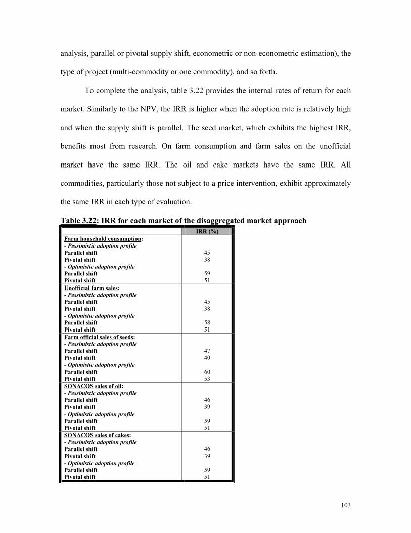
To complete the analysis, table 3.22 provides the internal rates of return for each

market. Similarly to the NPV, the IRR is higher when the adoption rate is relatively high

and when the supply shift is parallel. The seed market, which exhibits the highest IRR,

benefits most from research. On farm consumption and farm sales on the unofficial

market have the same IRR. The oil and cake markets have the same IRR. All

commodities, particularly those not subject to a price intervention, exhibit approximately

the same IRR in each type of evaluation.

Table 3.22: IRR for each market of the disaggregated market approach IRR (%)

Farm household consumption: - Pessimistic adoption profile Parallel shift Pivotal shift - Optimistic adoption profile Parallel shift Pivotal shift

45 38

59 51


45 38

58 51


47 40

60 53


46 39

59 51


46 39

59 51

103

3.3.3 Sensitivity analyses

In most circumstances, researchers are confronted with some uncertainty

regarding the parameters they use in their analyses. In this study, the parameter

uncertainty is due to several factors: parameter approximation, parameter estimation and

parameter variability from year to year.

Research costs were approximated in the absence of actual data. They were

approximated on the basis of salaries, which were augmented by a percentage to account

for operating costs. The study has been conducted so far on the basis of a 20 percent

increase, but a higher increase could also be considered given that in developing

countries the share of salaries in total research expenditures is likely to be relatively low.

For sensitivity analysis a 50 percent increase in research costs is considered. Table 3.23

contains the new research costs. The new annual research costs vary between 6 and 11

million CFA Francs.

Table 3.23: Estimated annual research costs on La Fleur 11 with a 50 percent increase of researcher salaries

Years Researcher salaries Research costs 1985 1986 1987 1988 1989 1990 1991 1992 1993 1994 1995 1996

4,170,612 4,170,612 4,170,612 4,170,612 4,267,086 4,363,560 7,269,768 7,269,768 7,367,752 7,890,768 7,467,984 7,467,984

6,255,918 6,255,918 6,255,918 6,255,918 6,400,629 6,545,340

10,904,652 10,904,652 11,051,628 11,836,152 11,201,976 11,201,976

Elasticities were estimated in previous studies. All the elasticities found in the

literature are short-run elasticities. Given that the present research evaluation is

conducted over more than three decades, using long-run elasticities may be more

appropriate. Accordingly, another evaluation is conducted using long-run elasticities. The

104

demand elasticity of –1.8 is arbitrarily chosen for the unshelled peanut market to replace

the elasticity of –0.18. The supply elasticity of 3 and the demand elasticity of -2 are

arbitrarily chosen for the oil and cake markets to replace the elasticities of 0.3 and –0.2

respectively. Concerning the elasticity of supply for unshelled peanuts, a unitary

elasticity is used. There are two reasons behind this choice. First, with a unitary elasticity

the gross cost reduction per unit of output ∆Y/Yε, the supply shift and research benefits

are neither under-estimated (as with a very elastic supply) nor over-estimated (as with a

very inelastic supply). Second, Gaye (1998 b) showed that the land use is very inelastic

with respect to the peanut price: 0.223. Therefore, it is likely that the supply elasticity of

unshelled peanuts is not very elastic in the long-run as well. A supply elasticity of 1

versus 0.77 may be enough to capture the effect of a relatively higher elasticity.

Only one number was used for the exchange rate (the average exchange rate for

1999, 615.70 CFA Francs/U.S. Dollar) and for the discount rate (the discount rate applied

after August 31st 1998, 0.0625). However, these parameters vary every year.

Consequently, instead of considering one-year’s information an average is calculated for

several years. For the exchange rate the post-devaluation period 1994-1999 is used in

order to have comparable exchange rates. For the discount rate, the period October 1993

through September 1998 is used to calculate an average of the interest rate applied in the

money market. The choice of this period is based on the availability of the data. The new

numbers used are 560.11 CFA Francs/U.S. Dollar for the exchange rate and 0.0559 for

the discount rate. The data used for the calculation of these averages were presented

earlier in tables 3.2 and 3.3.

105

Though prices and quantities vary from year to year, no sensitivity analysis is

conducted on these variables. The evaluation was conducted on the basis of averages as

suggested by Alston et al (1995).

New results are obtained for each parameter changed and compared to the

baseline scenario. For each parameter varied, only the most insightful results are

presented.

1/ Research costs

Table 3.24: Total research benefits net of research costs for the different evaluations with a 50 percent increase in research salaries


Pessimistic adoption profile 12,394,065.21 6,548,376.81 9,666,931.03 4,854,827.43 Optimistic adoption profile 32,029,525.97 16,576,210.32 25,620,383.66 12,899,391.59

In table 3.24, because research costs are higher compared to the baseline there is a

slight decrease in net benefits by $22,315.87 for the aggregated market scenario and by

$18,745.33 for the disaggregated market scenario for both types of adoption profiles and

supply shifts. These amounts are very low relative to the magnitude of the net benefits.

They represent less than 0.4 percent of the benefits: 0.18 percent for the pessimistic

adoption profile with the parallel shift; 0.3 percent for the pessimistic adoption profile

with the pivotal shift; 0.07 percent for the optimistic adoption profile with the parallel

shift; and 0.14 percent for the optimistic adoption profile with the pivotal shift. Therefore,

an increase in research costs doesn’t change the size of the benefits significantly.

106

2/ Supply and demand elasticities

Table 3.25: Distribution of total research benefits among consumers, producers, and the government for the different evaluations with long-run elasticities a) Pessimistic adoption profile:


Consumers 4,053,355.35 4,053,355.35 840,417.97 840,417.97 Producers 7,295,957.31 3,672,125.90 5,709,710.73 2,767,869.84 Government 4,092,584.78 4,092,584.78 613,887.72 613,887.72 Net social welfare 7,256,727.88 3,632,896.47 5,936,240.99 2,994,400.10

b) Optimistic adoption profile: Aggregated market scenario Disaggregated market scenario

US$ Parallel Pivotal Parallel Pivotal Consumers 10,807,471.14 10,807,471.14 2,238,743.04 2,238,743.04 Producers 19,452,947.87 9,873,201.77 15,291,255.98 7,514,379.64 Government 11,003,436.74 11,003,436.74 1,650,515.51 1,650,515.51 Net social welfare 19,256,982.28 9,677,236.18 15,879,483.51 8,102,607.17

In table 3.25, long-run elasticities change both the size and the distribution of

research benefits in comparison to short-run elasticities. In comparison to the baseline

scenario, all benefits and costs are lower. Consumers’ benefits decrease by 91 percent on

average. In the aggregated market scenario, producers’ benefits decrease by 38 percent.

In the disaggregated market scenario, producers’ benefits decrease by 34 percent with a

parallel shift and 29 percent with a pivotal shift. The increase in the cost of the subsidy

decreases by 92 percent. The change in net social welfare decreases by 42 percent on

average in the aggregated market scenario and 38 percent on average in the disaggregated

market scenario.

In comparison to the baseline scenario, producers are now the main beneficiaries.

In the aggregated market scenario, producers gain 80 percent more benefits than

consumers with the parallel supply shift and 9 percent less with the pivotal supply shift.

In the disaggregated market scenario, producers gain 6.8 times more surplus with the

parallel supply shift and 3.3 times more surplus with the pivotal supply shift than

107

consumers. Again, while consumers’ benefits don’t change with the type of supply shift,

producers’ benefits with a pivotal shift are about half those with a parallel shift. As

indicated by theory, producers benefit more from research when demand is relatively

elastic. With an elasticity of demand of –0.18 (versus a supply elasticity of 0.77),

producers were gaining 77 percent less surplus than consumers with a parallel supply

shift and 89 percent less surplus with a pivotal supply shift in the aggregated market

scenario. In the disaggregated market scenario, producers were gaining 3 percent more

surplus than consumers with the parallel supply shift but 53 percent less surplus with the

pivotal supply shift. With an elasticity of demand of –1.8 (versus a supply elasticity of 1),

producers’ change in surplus is greater than consumers’ in most evaluations.

In the aggregated market scenario, with a parallel supply shift the increase in the

cost of the subsidy represents 36 percent of the benefits to consumers and producers; the

remaining 54 percent are the increase in net social welfare. With a pivotal supply shift,

the increase in the cost of the subsidy and the increase in net social welfare represent 53

and 47 percent respectively of the total benefits to consumers and producers. In the

disaggregated market scenario, with a parallel supply shift the increase in the cost of the

subsidy represents 9 percent of the benefits to consumers and producers; the remaining

91 percent are the increase in net social welfare. With a pivotal supply shift, the increase

in the cost of the subsidy and the net social welfare represent 17 and 83 percent

respectively of the total benefits to consumers and producers. Therefore, with long-run

elasticities the increase in the cost of the subsidy is lower and the increase in net social

welfare is higher relative to the gross social benefits. This result is known in economic

theory; government interventions generate fewer losses in relatively elastic markets.

108

For a complete analysis of the impact of long-run elasticities on the distribution

and the size of the benefits, it would be insightful to look at the different markets that

compose the disaggregated market scenario. Table 3.26 contains the impact of long-run

elasticities on the distribution and the size of research benefits for each market.

109

Table 3.26: Impact of long-run elasticities on the distribution and size of the benefits in the disaggregated market scenario

US$ Total* Consumers Producers Government Farm household consumption: - Pessimistic adoption profile Parallel shift Pivotal shift - Optimistic adoption profile Parallel shift Pivotal shift

1,611,719.52 805,859.76

4,260,646.28 2,130,323.14

1,611,719.52 805,859.76

4,260,646.28 2,130,323.14


650,761.08 326,695.66

1,729,342.65

872,662.50

232,414.67 232,414.67

617,622.37 617,622.37

418,346.41 94,280.99

1,111,720.27

255,040.12


1,088,509.18 544,934.47

2,888,547.34 1,451,585.43

608,003.30 608,003.30

1,621,120.67 1,621,120.67

1,094,393.60 550,818.89

2,917,942.18 1,480,980.27

613,887.72 613,887.72

1,650,515.51 1,650,515.51

Farm level: - Pessimistic adoption profile Parallel shift Pivotal shift - Optimistic adoption profile Parallel shift Pivotal shift

3,350,989.78 1,677,489.89

8,878,536.27 4,454,571.06

840,417.97 840,417.97

2,238,743.04 2,238,743.04

3,124,459.53 1,450,959.64

8,290,308.73 3,866,343.53

613,887.72 613,887.72

1,650,515.51 1,650,515.51


1,275,638.54 641,468.04

3,397,253.79 1,720,798.22

1,275,638.54 641,468.04

3,397,253.79 1,720,798.22


1,309,612.66 675,442.17

3,603,693.46 1,927,237.89

1,309,612.66 675,442.17

3,603,693.46 1,927,237.89

SONACOS level: - Pessimistic adoption profile Parallel shift Pivotal shift - Optimistic adoption profile Parallel shift Pivotal shift

2,585,251.20 1,316,910.21

7,000,947.25 3,648,036.11

2,585,251.20 1,316,910.21

7,000,947.25 3,648,036.11

*: Some totals may not correspond to the exact sum of consumer surplus, producer surplus and change in the government cost of subsidy due to rounding errors.

110

In table 3.26, in comparison to the baseline scenario, research benefits decrease

by 40 percent at the farm level and 35 percent at the SONACOS level. Benefits from

farm household consumption decrease by 39 percent. Benefits from farm sales on the

unofficial market decrease by 41 percent. Benefits from the official seed market decrease

by 42 percent. At the farm-level, consumers’ benefits decrease by 90 percent and

producers’ benefits decrease by 32 percent with a parallel shift and 23 percent with a

pivotal shift. The decrease with the pivotal shift is mostly due to farm household

consumption. With the pivotal shift, producer surplus from unofficial farm sales increases

with long-run elasticities while it decreases with short-run elasticities. The government

cost of the subsidy increases but by 91 percent less than in the baseline scenario.

At the SONACOS level, research benefits decrease by 37 percent in the oil

market and about 34 percent in the cake market. Producers’ benefits decrease by 35

percent.

In conclusion, in comparison to the baseline scenario long-run elasticities change

the magnitude and the distribution of research benefits. They decrease consumers’ and

producers’ research benefits, the government cost of the subsidy, and the net social

welfare. Therefore, only the government benefits from long-run elasticities versus short-

run elasticities. The distribution of research benefits is more beneficial to producers than

consumers in the aggregated market scenario (parallel shift) and at both levels (farmers’

and SONACOS’) of the disaggregated market scenario than in the baseline scenario.

111

3/ Exchange rate

Table 3.27: Total research benefits net of research costs for the different evaluations with an average exchange rate



In table 3.27, since the change in the exchange rate applies equally to the different

components of each evaluation (change in consumer surplus, change in producer surplus

and change in the government cost of the subsidy), it doesn’t affect the distribution of the

benefits among consumers, producers and the government. However, the size of research

benefits is higher because a lower exchange rate is employed. A decrease in exchange

rate by 9 percent causes research benefits to increase by 9.9 percent in comparison to the

baseline scenario.

4/ Discount rate

Table 3.28: Total research benefits net of research costs for the different evaluations with an average discount rate



In table 3.28, since the change in the discount rate applies equally to the different

components of each evaluation (change in consumer surplus, change in producer surplus

and change in the government cost of the subsidy), it doesn’t affect the distribution of the

benefits among consumers, producers and the government. However, the size of research

benefits is higher since a lower discount rate is employed. A decrease in the discount rate

by 10 percent causes research benefits to increase by 16 percent with the pessimistic

adoption profile and 15 percent with the optimistic adoption profile in comparison to the

baseline scenario.

112

3.3.4 Conclusion

Benefits from the adoption of La Fleur 11 are positive. However, no general

conclusion can be drawn about the distribution of research benefits among consumers,

producers and the government. This depends on the type of procedure considered

aggregated market or disaggregated market, on the type of commodity-market, on the

level where the evaluation is done, and so forth. The aggregated market scenario (which

is also a closed economy scenario) is more favorable to consumers than producers. The

disaggregated market scenario is more favorable to producers with the parallel supply

shift and more favorable to consumers with the pivotal supply shift. Consumers only

benefit from closed economy markets and farm level evaluations. Producers benefit from

all markets. Pricing policies change the size and the distribution of research benefits

drastically. Consumers are the main beneficiaries from the implementation of a producer

base price. Producers benefit mainly from household consumption, which represents a

large proportion of the supply, and oil and cake exports at the world price. Research

increases the government cost of the subsidy in the markets where a producer base price

is implemented (aggregated market and seed market). Most of these results were

predicted by theory.

The results of sensitivity analysis show that a change in research costs, the

exchange rate and the discount rate don’t affect the distribution of research benefits but

they do affect the size of research benefits in comparison to the baseline scenario.

Research benefits decrease with higher research costs and increase with lower exchange

rate and discount rate. When long-run elasticities replace short-run elasticities, both the

size and the distribution of research benefits are affected. Consumers and producers

113

benefit less from research in all evaluations with long-run elasticities. With long-run

elasticities, the distribution of research benefits is generally more favorable to producers

than consumers (because demand is more elastic than supply). The government is the

only beneficiary from long-run elasticities as it pays less for the subsidy.

114

Documents

CHAPTER 3: DATA AND RESULTS