Chapter 23 WAVE EQUATION

• Introduction• Wave-particle duality• Quantized modes• Schrödinger equation• One-dimensional solutions• Three-dimensional solutions• Dirac Equation• Conclusions

INTRODUCTION

de Broglie’s 1923 hypothesis of wave-particle duality,

was the key idea that led to the development of quan-

tum mechanics. The basis of quantum mechanics was

developed in an incredible spurt of advances during

1926. It is fascinating to see how quickly things devel-

oped and how much trouble even the greatest minds

had in accepting some of these new ideas. Many of the

scientists involved had a spark of genius and then faded

from sight. Schrödinger’s development of his wave

equation was a tremendous step forward. Heisenberg

developed quantum mechanics via his matrix mechan-

ics methods which use abstract mathematical methods

that do not provide the intuition that wave mechan-

ics can provide. However, practicing physicists actu-

ally use the Heisenberg matrix mechanics because it is

more powerful. The story of the development of quan-

tum mechanics is interesting. Schrödinger had a rep-

utation of being a playboy, or as Einstein called him,

a clever rogue. Many of these physicists migrated to

the US in the late 1930’s, because of the rise of the

Nazis in Germany, and they contributed significantly

to advancing science in the US as well as development

of nuclear power and the bomb. Heisenberg was a

member of the German Youth movement and stayed

in Germany playing a role in the German nuclear bomb

project during World War 2.

The application of quantum mechanics requires de-

velopment of a wave equation. In contrast to classical

physics, where the wave equation can be derived from

first principles, this discussion will resort to plausibil-

ity arguments to develop a useful wave equation. This

chapter will review the wavefunction and the Copen-

hagen interpretation of matter waves before discussing

the non-relativistic Schrödinger wave equation and ap-

plications. This will be followed by a brief description

of the relativistic Dirac equation.

WAVE-PARTICLE DUALITY

Wavefunction

In wave mechanics one deals with the amplitude of

the matter waves. The amplitude of the matter wave

is usually written as a greek letter psi, Ψ which is a

function of x,y,z, and time. This is analogous to waves

on a string where, at any instant in time, we can write

down the amplitude of the string displacement as a

function of location on the string. The mathematics

of waves is simpler using complex numbers, rather than

sine and cosine functions to describe wavefunctions.

= (cos + sin )

It is much easier to add or subtract exponents of the

exponentials rather than take products of sines and

cosines.

The real part of projects out , while the

imaginary part projects out the corresponding sin

function. The simplest travelling wave in one dimen-

sion, of the form

Ψ = cos(− )

can be rewritten in the exponential form as:

Ψ = (−)

The wavefunction can comprise a range of values for

and For matter waves, and are given by the

de Broglie relations, that is, the relativistic energy

E = ~

and the component of the linear momentum

= ~

Copenhagen interpretation

The Copenhagen Interpretation of wave-particle du-

ality is that the intensity of the wave, |Ψ( )|2gives the probability distribution function () of

finding the particle at any location, x,y,z, at time t.

That is

() = |Ψ()|2

Quantum mechanics is probabilistic, that is, it does

not determine the exact behavior of the particle, it

only tells you the probability of finding the particle

with certain conditions. Assuming that the probability

175

of finding the particle somewhere is unity, implies that

the integral of the probability over all space is unity.Z

|Ψ|2 = 1

As discussed last time, the idea that nature is basically

probabilistic, even for a single particle, was philosphi-

cally unacceptable to many physicists. It ran counter

to the deterministic approach so successfully applied in

classical physics. Last lecture discussed the double-slit

interference pattern as an example where the predicted

intensity of the wave gave the probability distribution

of detecting individual photons.

Expectation values

Wave motion implies that exact specifications for a

particle cannot be determined simultaneously, only the

probability distribution is measureable. Thus one can

only determine expectation values, that is average val-

ues, for observables. For example the average value of

position x is given by evaluating the probability dis-

tribution with x,. That is, the expectation value of x

is;

hi =Z

|Ψ( )|2

Similarly one can evaluate the expectation value for

x2; ­2®=

Z2 |Ψ( )|2

These can be used to calculate the standard deviation

of the spread of the average value That is;

() =p( 2 −( )2)

Note that () is a non-zero positive number for a

non-localized probability distribution.

The expectation values of time, linear momentum,

angular momentum, energy, or other possible observ-

ables can be evaluated if the wavefunction is known,

providing a method for relating physical observables

in quantum physics.

Uncertainty principle

As discussed last lecture, the Uncertainty Principle ap-

plies to all forms of wave motion, be it sound waves,

water waves, electromagnetic waves, or de Broglie mat-

ter waves. Namely for the wave intensity, the standard

deviations for measurements of conjugate variables,

that is related variables, have a minimum product of

the uncertainties:

() · () ≥ 12

() · () ≥ 12

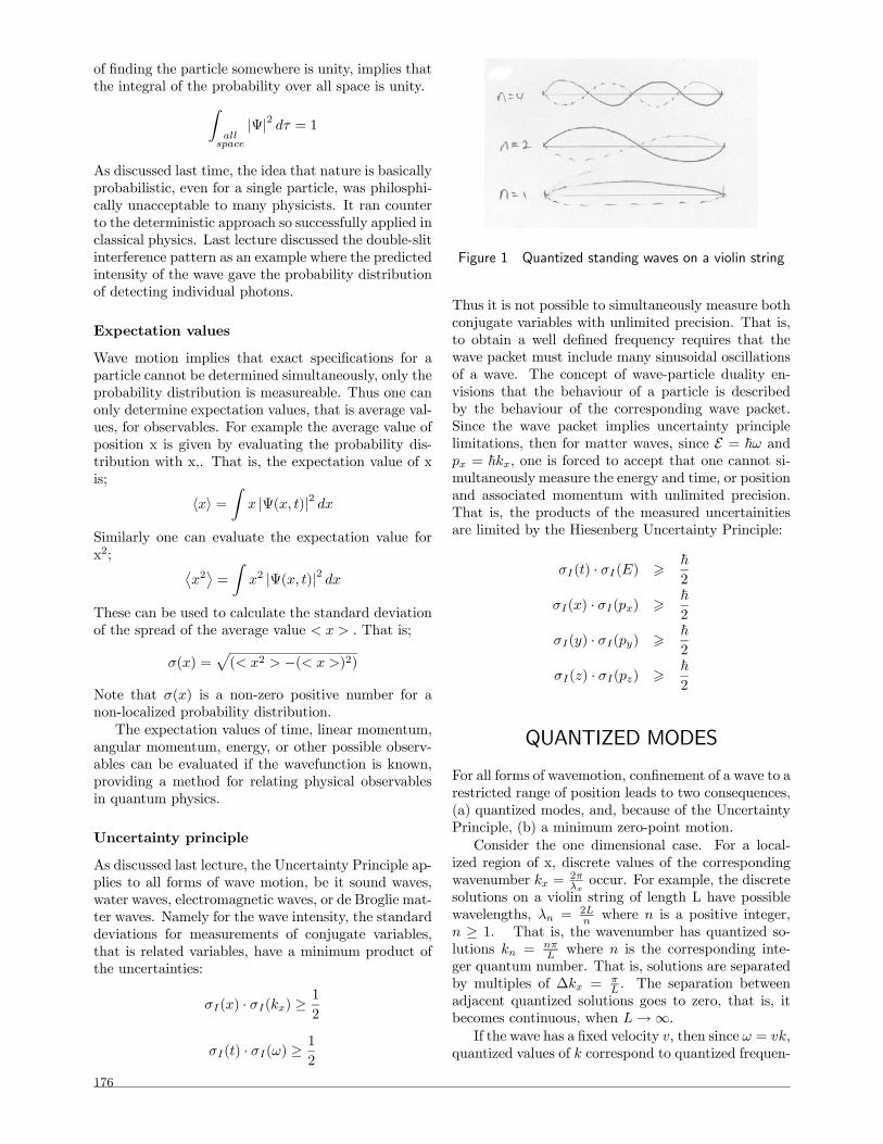
Figure 1 Quantized standing waves on a violin string

Thus it is not possible to simultaneously measure both

conjugate variables with unlimited precision. That is,

to obtain a well defined frequency requires that the

wave packet must include many sinusoidal oscillations

of a wave. The concept of wave-particle duality en-

visions that the behaviour of a particle is described

by the behaviour of the corresponding wave packet.

Since the wave packet implies uncertainty principle

limitations, then for matter waves, since E = ~ and = ~ one is forced to accept that one cannot si-multaneously measure the energy and time, or position

and associated momentum with unlimited precision.

That is, the products of the measured uncertainities

are limited by the Hiesenberg Uncertainty Principle:

() · () > ~2

() · () > ~2

() · () > ~2

() · () > ~2

QUANTIZED MODES

For all forms of wavemotion, confinement of a wave to a

restricted range of position leads to two consequences,

(a) quantized modes, and, because of the Uncertainty

Principle, (b) a minimum zero-point motion.

Consider the one dimensional case. For a local-

ized region of x, discrete values of the corresponding

wavenumber =2occur. For example, the discrete

solutions on a violin string of length L have possible

wavelengths, =2where is a positive integer,

≥ 1. That is, the wavenumber has quantized so-

lutions =where is the corresponding inte-

ger quantum number. That is, solutions are separated

by multiples of ∆ =. The separation between

adjacent quantized solutions goes to zero, that is, it

becomes continuous, when →∞

If the wave has a fixed velocity , then since = ,

quantized values of correspond to quantized frequen-

176

cies . For matter waves, quantized values of im-

plies quantized = ~, and consequently quantizedvalues of kinetic energy.

A one-dimensional wave leads to a single integer

quantum number n characterizing the solutions. A

three-dimensional box can have three independent stand-

ing waves for each independent degree of freedom, i.e.

the x, y, and z directions. Standing wave systems for

each of these three independent spatial degrees of free-

dom has an associated quantum number characterizing

the number of half wavelengths fitting along that di-

mension. Thus there is one quantum number for every

degree of freedom of a quantal system.

Last lecture is was shown that the Heisenberg Un-

certainty principle implies that for any particle con-

fined within a localized region, there is a corresponding

zero-point kinetic energy which is the minimum energy

allowed for a particle of mass m confined within this

region. Thus even the lowest state of a system having

a localized particle, has a minimum kinetic energy.

These conclusions are properties of waves in gen-

eral and are manifest by matter waves as discussed.

More specific discussion of quantum theory requires

development of a wave equation.

SCHRÖDINGER EQUATION

Although Heisenberg’s matrix mechanics was devel-

oped first, the Schrödinger equation was the first use-

ful quantum wave equation. However, the Schrödinger

equation is applicable only to non-relativistic cases. As

opposed to classical physics, where the wave equa-

tion can be derived from first principles, in quantum

physics the wave equation is obtained by a plausibility

argument based on classical physics and the de Broglie

hypotheses. Inserting the de Broglie relations

E = ~

= ~

into the simplest form of a travelling wave in one di-

mension gives:

Ψ0 = (−) = ~ (−E)

The relativistic energy E = +2 where is the

kinetic energy. The wave function can be written as

Ψ0 = ~ (−E)−

~

2 = Ψ−~

2

where

Ψ = ~ (−)

The exponential term −~

2 can be ignored, since

it only introduces an unimportant phase factor that

has no influence on the probability, that is,

|Ψ0|2 = |Ψ|2

Consider the wavefunction Ψ( ) in one dimen-

sion. Note that differentials of Ψ( ) are:

Ψ

= −

~Ψ

That is:

Ψ = ~Ψ

Also:2Ψ

2= −

2

~2Ψ

That is:

2Ψ = −~22Ψ

2

Time-dependent Schrödinger equation

Schrödinger developed a non-relativistic wave equation

based on the fact that:

=2

2+

where U is the potential energy. Since¡

¢2is 10−5 for

electron orbits in atoms, and 10−3 for protons in thenucleus, the non-relativistic equation is a reasonable

approximation for solving many problems in atomic

and nuclear physics.

Substituting the above differential expressions for

E and 2 = 2 + 2 + 2, gives Schrödinger’s time-

dependent equation in three dimensions:

Ψ = ~Ψ

= − ~

2

2

µ2Ψ

2+

2Ψ

2+

2Ψ

2

¶+ Ψ

(Time dependent Schrodinger equation)

Note that the following facts were used in develop-

ing this equation:

• de Broglie-Einstein relations E = ~ −→p = ~−→k

• Non-relativistic relation = 2

2+

• Ignored consequences of the phase factor − ~

2

In general the wavefunction Ψ( ) is obtained

by solving this time-dependent equation for some known

potential ( )

Time-independent Schrödinger equation.

A frequently encountered problem is where the po-

tential is time independent, ( ) for which the

quantized energy solutions are time independent. For

such cases the right-hand side of the time-dependent

Schrödinger equation is a function of only the spatial

coordinates while the left-hand side is a function only

of time. For such a system the two sides are indepen-

dent and the spatial and time parts of the wavefunction

can be separated:

Ψ( ) = ( )−~

177

The left-hand side of the equation equals:

~Ψ

= ~

−~

= Ψ

while the right-hand side gives:

= − ~2

2

µ2

2+

2

2+

2

2

¶+

(Time independent Schrodinger equation)

where the time-dependent term of Ψ, that is, −~

on both sides cancels. This equation is easier to solve

than is Schrödinger’s time-dependent equation.

The solution of the Schrödinger equation must sat-

isfy the following restrictions.

Wavefunction normalization

The wavefunction must be correctly normalized,

that is the probability of finding the particle over all

space must be unity, that is:Z

||2 = 1 (Wavefunction normalization.)

This fixes the normalization of the wavefunction.

Continuity

The wavefunction must be a well-behaved function

for which Ψ,

22

22

and 22

all exist. This implies

that:

is continuous−→∇ is continuous

That is,

and

all are continuous, if the po-

tential energy function is not infinite.

ONE-DIMENSIONAL SOLUTIONS

Schrödinger’s equation is easiest to understand by con-

sidering problems in one-dimension.

Infinite square well

Consider a mass m contained in a one-dimensional box

with = 0 for 0 ≤ ≤ and = ∞ outside this

region. The time independent Schrödinger equation

for 0 ≤ ≤ is:

− ~2

2

2

2=

since = 0 The wavefunction must be zero outside

of the box because then the potential = ∞ Thus

() must equal zero at the walls of the box, = 0

and = . Therefore, as for waves on a violin string,

the solutions of = sin() for 0 ≤ ≤ are:

= sin() =

r2

sin³

´

Figure 2 Infinite one-dimensional box. The spatial

dependence of and excitation energies E are shown

for = 1 2 3.

where n is an integer quantum number. The constant

A has been normalized by requiringR 02 = 1

while the wavenumber is given by:

=2

=

that is,

=2

Substitution of into the Schrödinger equation

gives corresponding energies:

=~2

22 = 2

~22

22

These are the allowed energies E corresponding to the

wavefunction for each quantum number Figure

2 shows the energies, which are proportional to 2

and the corresponding wavefunctions. Note that the

lowest state has n=1 giving an energy 1 =~22

22

This is greater than the minimum zero-point energy

given by the Heisenberg uncertainty principle.

Finite square well

Consider the potential well shown in figure 3, where

= 0 for 0 ≤ ≤ = outside of this region of

. Thus the Schrödinger equation can be written as:

− ~2

2

2

2= (0 ≤ ≤ )

− ~2

2

2

2= ( − ) ( ≤ 0 or ≥ )

178

Figure 3 Particle in a finite square potential well.

Consider possible standing-wave solutions of the

form:

= +−

Inserting this into the Schrödinger equation gives

inside the potential well, 0 ≤ ≤

~2

22 =

and outside the well:

~2

220 = −

Thus the solution inside the well is a sinusoidal stand-

ing wave with wavenumber:

=

√2

~(Wavenumber inside well)

That is:

= +− = sin()

The wavenumber outside of the well is given by:

0 =

p2( − )

~(Wavenumber outside well.)

Note that if − is positive, that is exceeds the

depth of the potential, then the solution is sinusoidal

with a smaller wavenumber, that is longer wavelength,

than inside the potential well. If − is negative,

that is, thenp2( − ) is an imaginary

number. That is:

0 =p2( −)

~=

Thus the solution outside the well now is:

= − +

This corresponds to an exponential decay as shown in

figure 3.

The final solutions inside and outside of the well are

now obtained using the continuity and normalization

requirements, that is:

Figure 4 The potential energy, energy and wavefunction

distributions for a binding of a diatomic molecule.

• Matching the inside and outside values of atthe well boundaries = 0 and = .

• Matching the inside and outside gradients at

the well boundaries = 0 and = .

• Requiring that R∞−∞ ||2 = 1Note that for , we seem to violate classical

physics by having a finite probability of finding the

particle with negative kinetic energy. However, it can

be shown that, because of the Heisenberg uncertainty

principle, it is not possible to measure this negative

kinetic energy outside of the potential well.

This exponential decay of the wavefunction in classically-

forbidden regions is a common feature in quantum

physics. For example, a plot of the potential energy

versus separation distance due to binding of a diatomic

molecule is close to that of a one-dimensional harmonic

oscillator shown in figure 4. Solutions in this well are

illustrated in figure 4. For a large quantum number

the greatest probability occurs with the diatomic hav-

ing maximum separation distance just as is obtained

for a harmonic oscillator such as the pendulum.

THREE-DIMENSIONAL SOLUTIONS

Solution of the time-independent Schrödinger equation

in three dimensions leads to solutions in three inde-

pendent directions, each of which has its own quan-

tum number. It is useful to first consider the three-

dimensional infinite square well potential since it il-

lustrates important characteristics of solutions of the

Schrödinger equation.

179

THREE DIMENSIONAL INFINITE SQUARE

WELL

Consider the three-dimensional infinite square well po-

tential where () = 0 for 0 0 ,

0 Outside this cubical square well () =

∞ The wave function solutions to this potential must

be zero at the infinite boundaries. Thus the solutions

inside the box are of the form

Ψ() = sin 1 sin 2 sin 3

where the constant A is given by normalization of the

wavefunction. Inserting this solution into Schrödinger’s

equation gives energies inside the box of

=~2

2

¡21 + 22 + 23

¢As for the infinite one-dimensional square well, the po-

tential must be zero at the walls, therefore the only

possible solutions are quantized with

1 = 1

2 = 2

3 = 3

where ≥ 1 and integer. Therefore

=~22

22

¡21 + 22 + 23

¢The lowest energy, that is, ground state, for this

cubical infinite square well is

111 =3~22

22

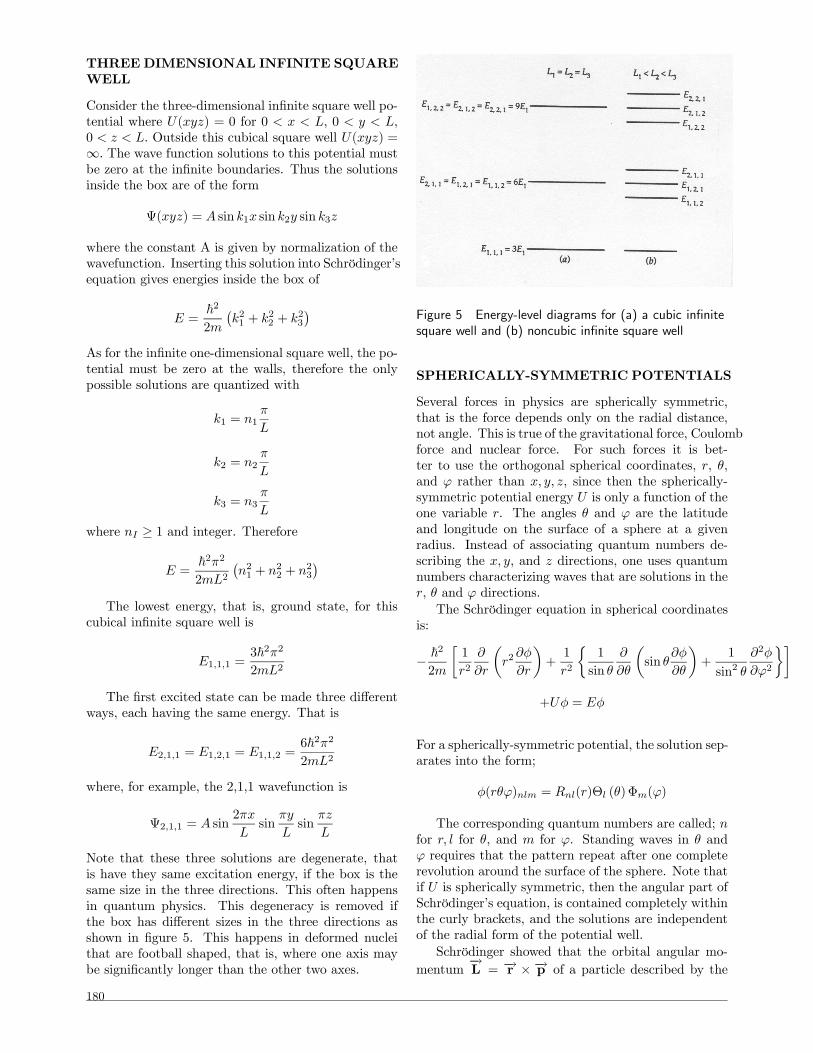
The first excited state can be made three different

ways, each having the same energy. That is

211 = 121 = 112 =6~22

22

where, for example, the 2,1,1 wavefunction is

Ψ211 = sin2

sin

sin

Note that these three solutions are degenerate, that

is have they same excitation energy, if the box is the

same size in the three directions. This often happens

in quantum physics. This degeneracy is removed if

the box has different sizes in the three directions as

shown in figure 5. This happens in deformed nuclei

that are football shaped, that is, where one axis may

be significantly longer than the other two axes.

Figure 5 Energy-level diagrams for (a) a cubic infinite

square well and (b) noncubic infinite square well

SPHERICALLY-SYMMETRIC POTENTIALS

Several forces in physics are spherically symmetric,

that is the force depends only on the radial distance,

not angle. This is true of the gravitational force, Coulomb

force and nuclear force. For such forces it is bet-

ter to use the orthogonal spherical coordinates, , ,

and rather than , since then the spherically-

symmetric potential energy is only a function of the

one variable . The angles and are the latitude

and longitude on the surface of a sphere at a given

radius. Instead of associating quantum numbers de-

scribing the and directions, one uses quantum

numbers characterizing waves that are solutions in the

, and directions.

The Schrödinger equation in spherical coordinates

is:

− ~2

2

∙1

2

µ2

¶+1

2

½1

sin

µsin

¶+

1

sin2

2

2

¾¸+ =

For a spherically-symmetric potential, the solution sep-

arates into the form;

() = ()Θ ()Φ()

The corresponding quantum numbers are called;

for for , and for . Standing waves in and

requires that the pattern repeat after one complete

revolution around the surface of the sphere. Note that

if is spherically symmetric, then the angular part of

Schrödinger’s equation, is contained completely within

the curly brackets, and the solutions are independent

of the radial form of the potential well.

Schrödinger showed that the orbital angular mo-

mentum−→L = −→r × −→p of a particle described by the

180

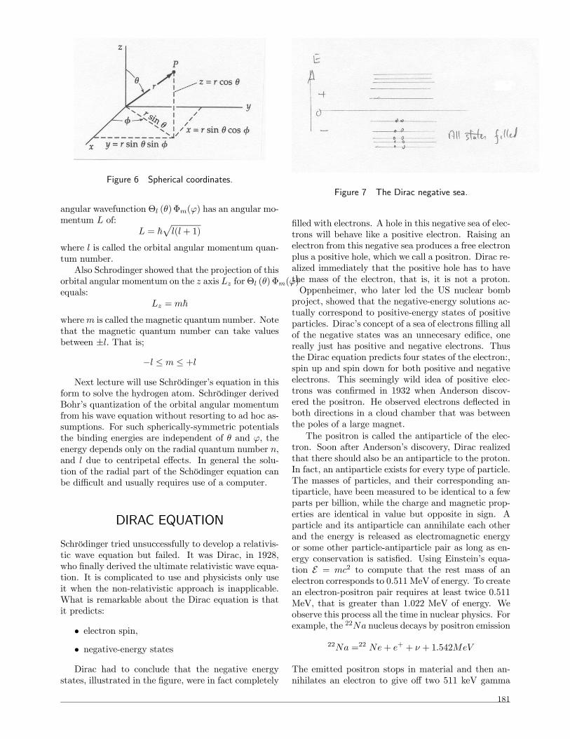
Figure 6 Spherical coordinates.

angular wavefunction Θ ()Φ() has an angular mo-

mentum of:

= ~p( + 1)

where is called the orbital angular momentum quan-

tum number.

Also Schrodinger showed that the projection of this

orbital angular momentum on the axis forΘ ()Φ()

equals:

= ~

where is called the magnetic quantum number. Note

that the magnetic quantum number can take values

between ± That is;

− ≤ ≤ +

Next lecture will use Schrödinger’s equation in this

form to solve the hydrogen atom. Schrödinger derived

Bohr’s quantization of the orbital angular momentum

from his wave equation without resorting to ad hoc as-

sumptions. For such spherically-symmetric potentials

the binding energies are independent of and the

energy depends only on the radial quantum number ,

and due to centripetal effects. In general the solu-

tion of the radial part of the Schödinger equation can

be difficult and usually requires use of a computer.

DIRAC EQUATION

Schrödinger tried unsuccessfully to develop a relativis-

tic wave equation but failed. It was Dirac, in 1928,

who finally derived the ultimate relativistic wave equa-

tion. It is complicated to use and physicists only use

it when the non-relativistic approach is inapplicable.

What is remarkable about the Dirac equation is that

it predicts:

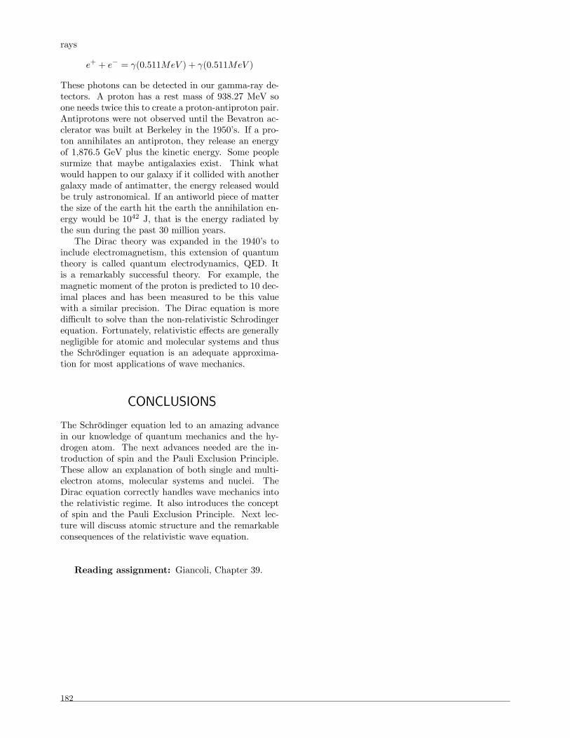
• electron spin,• negative-energy states

Dirac had to conclude that the negative energy

states, illustrated in the figure, were in fact completely

Figure 7 The Dirac negative sea.

filled with electrons. A hole in this negative sea of elec-

trons will behave like a positive electron. Raising an

electron from this negative sea produces a free electron

plus a positive hole, which we call a positron. Dirac re-

alized immediately that the positive hole has to have

the mass of the electron, that is, it is not a proton.

Oppenheimer, who later led the US nuclear bomb

project, showed that the negative-energy solutions ac-

tually correspond to positive-energy states of positive

particles. Dirac’s concept of a sea of electrons filling all

of the negative states was an unnecesary edifice, one

really just has positive and negative electrons. Thus

the Dirac equation predicts four states of the electron:,

spin up and spin down for both positive and negative

electrons. This seemingly wild idea of positive elec-

trons was confirmed in 1932 when Anderson discov-

ered the positron. He observed electrons deflected in

both directions in a cloud chamber that was between

the poles of a large magnet.

The positron is called the antiparticle of the elec-

tron. Soon after Anderson’s discovery, Dirac realized

that there should also be an antiparticle to the proton.

In fact, an antiparticle exists for every type of particle.

The masses of particles, and their corresponding an-

tiparticle, have been measured to be identical to a few

parts per billion, while the charge and magnetic prop-

erties are identical in value but opposite in sign. A

particle and its antiparticle can annihilate each other

and the energy is released as electromagnetic energy

or some other particle-antiparticle pair as long as en-

ergy conservation is satisfied. Using Einstein’s equa-

tion E = 2 to compute that the rest mass of an

electron corresponds to 0.511 MeV of energy. To create

an electron-positron pair requires at least twice 0.511

MeV, that is greater than 1.022 MeV of energy. We

observe this process all the time in nuclear physics. For

example, the 22 nucleus decays by positron emission

22 =22 + + + + 1542

The emitted positron stops in material and then an-

nihilates an electron to give off two 511 keV gamma

181

rays

+ + − = (0511 ) + (0511 )

These photons can be detected in our gamma-ray de-

tectors. A proton has a rest mass of 938.27 MeV so

one needs twice this to create a proton-antiproton pair.

Antiprotons were not observed until the Bevatron ac-

clerator was built at Berkeley in the 1950’s. If a pro-

ton annihilates an antiproton, they release an energy

of 1,876.5 GeV plus the kinetic energy. Some people

surmize that maybe antigalaxies exist. Think what

would happen to our galaxy if it collided with another

galaxy made of antimatter, the energy released would

be truly astronomical. If an antiworld piece of matter

the size of the earth hit the earth the annihilation en-

ergy would be 1042 J, that is the energy radiated by

the sun during the past 30 million years.

The Dirac theory was expanded in the 1940’s to

include electromagnetism, this extension of quantum

theory is called quantum electrodynamics, QED. It

is a remarkably successful theory. For example, the

magnetic moment of the proton is predicted to 10 dec-

imal places and has been measured to be this value

with a similar precision. The Dirac equation is more

difficult to solve than the non-relativistic Schrodinger

equation. Fortunately, relativistic effects are generally

negligible for atomic and molecular systems and thus

the Schrödinger equation is an adequate approxima-

tion for most applications of wave mechanics.

CONCLUSIONS

The Schrödinger equation led to an amazing advance

in our knowledge of quantum mechanics and the hy-

drogen atom. The next advances needed are the in-

troduction of spin and the Pauli Exclusion Principle.

These allow an explanation of both single and multi-

electron atoms, molecular systems and nuclei. The

Dirac equation correctly handles wave mechanics into

the relativistic regime. It also introduces the concept

of spin and the Pauli Exclusion Principle. Next lec-

ture will discuss atomic structure and the remarkable

consequences of the relativistic wave equation.

Reading assignment: Giancoli, Chapter 39.

182