1

Chapter 2. Turbulence and the Planetary Boundary Layer In the chapter we will first have a qualitative overview of the PBL then learn the concept of Reynolds averaging and derive the Reynolds averaged equations. Making use of the equations, we will discuss several applications of the boundary layer theories, including the development of mixed layer as a pre-conditioner of server convection, the development of Ekman spiral wind profile and the Ekman pumping effect, low-level jet and dryline phenomena. The emphasis is on the applications. What is turbulence, really? Typically a flow is said to be turbulent when it exhibits highly irregular or chaotic, quasi-random motion spanning a continuous spectrum of time and space scales. The definition of turbulence can be, however, application dependent. E.g., cumulus convection can be organized at the relatively small scales, but may appear turbulent in the context of global circulations. Main references: Stull, R. B., 1988: An Introduction to Boundary Layer Meteorology. Kluwer Academic, 666 pp. Chapter 5 of Holton, J. R., 1992: An Introduction to Dynamic Meteorology. Academic Press, New York, 511 pp.

2.1. Planetary boundary layer and its structure The planetary boundary layer (PBL) is defined as the part of the atmosphere that is strongly influenced directly by the presence of the surface of the earth, and responds to surface forcings with a timescale of about an hour or less.

2

PBL is special because:

• we live in it • it is where and how most of the solar heating gets into the atmosphere • it is complicated due to the processes of the ground (boundary) • boundary layer is very turbulent • others … (read Stull handout).

In this section, we give a qualitative description of the planetary boundary layer.

3

Day time boundary layer is usually very turbulent, due to ground-level heating, as illustrated by the following figure.

4

The layer above the PBL is referred to as the free atmosphere.

• There is a strong diurnal variation in near-ground air temperature, and the amplitude of variation decreases with height

• Most of solar radiation is absorbed by the ground, which then

transfers the heat to the air via surface heat fluxes. The heat is further transported up via turbulence eddies (thermal plumes).

5

• Boundary wind can be divided into three parts: mean wind, waves

and turbulence, as illustrated by the above figure.

• All three parts can coexist and the total wind is then the sum of all three parts

• In the boundary layer, horizontal transport is dominated by the mean wind and vertical by the turbulence.

• A common approach to study turbulence is to split the variables, such as wind speed, temperature and mixing ratio into the mean and perturbation part, with the latter representing turbulent part.

6

7

• PBL is usually shallower in the high-pressure regions due to descending motion above, pushing the PBL top down. PBL horizontal divergence also decreases the height

• In the low-pressure region, PBL tend to be deeper, due to ascending

motion.

• When the ascent lifts the surface air parcel above the LCL, deep cumulus clouds can develop. In this case, it is hard to define the top of boundary layer. It is usually the subcloud layer that is studied most by boundary-layer meteorologists.

• The surface heating and the deepening of the daytime boundary layer is very relevant to thunderstorm forecast.

8

• The above figure shows the typical diurnal evolution of the BL in high-pressure regions (i.e., without the development of deep cumulus convection and much effect of vertical lifting).

• At and shortly after sunrise, surface heating causes turbulent eddies to develop,

producing a mixed layer whose depth grows to a maximum depth in late morning. In this mixed layer, potential temperature and water vapor mixing ratio are nearly uniform.

• At the sunset, the deep surface cooling creates a stable (nocturnal) boundary

layer, above which is a residual layer, basically the leftover part of the daytime mixed layer

• At all time, near the surface is a thin surface layer in which the vertical fluxes are

nearly constant. It is also called constant-flux layer.

9

• Turbulence in the mixed layer is usually convectively driven, i.e.,

driven by buoyancy due to instability

• Strong wind shear can also generate turbulence, however.

• The virtual potential temperature (it determines the buoyancy) is nearly adiabatic (i.e., constant with height) in the middle portion of the mixed layer (ML), and is super-adiabatic in the surface layer. At the top of the ML there is usually a stable layer to stop the turbulent eddies from rising further. When the layer is very stable so that the temperature increases with height, it is usually called capping inversion. This capping inversion can keep deep convection from developing.

• When the surface heating is sufficient so that the potential temperature

of the entire ML is raised above the maximum potential temperature of the capping inversion, convection breaks out (assuming there is sufficient moisture in the BL). This usually occurs in the later afternoon. The best time for tornado chasing.

• The boundary layer wind is usually sub-geostrophic, due to surface drag and vertical mixing of momentum.

• The water vapor mixing ratio is nearly constant in the ML.

10

An example of a deep well mixing boundary layer in the Front range area of the Rockies, shown in Skew-T diagram.

11

An example morning sounding showing the surface inversion (stable) layer that developed due to night-time surface cooling. Such a shallow stable layer

can usually be quickly removed after sunrise.

Assignment – Read Chapter 1 of Stull.

12

2.2. Reynolds averaging and Reynolds averaged equations We will study several aspects of the PBL. Before that, we need to develop a set of equations that are suitable for studying turbulent flows.

2.2.1. Reynolds Averaging (Holton p.119).

A time series plot of the wind speed can look like the above. There are many high-frequency (fast) fluctuations Such fluctuations are due to small turbulent eddies, and they do not reliably represent the mean flow To obtain a wind speed measurement representative of the large-scale flow, we obtain take an average over a time period long enough to smooth over the fluctuations but still short enough for keep the trend. The trend can be early identified in the above.

13

Such averaging was first proposed by Reynolds, and is therefore named after him. We use overbar to denote the mean value and prime to denote the perturbation. For any quantity A (could be e.g., vertical velocity w and potential temperature θ), we have 'A A A= +

where 0

1( , )

TA A x t dt

T= ∫ (2.1)

for a continuous function A, or

1

1( )

N

nn

A A xN =

= ∑ (2.2)

if we have discrete values of A. Here N is the number of points in the time series in time the chosen time interval T. Note that ( ) can be thought of as the integration operator, thus we can apply it as follows: ( ) ( ') ' 'A A A A A A A= + = + = + à ' 0A = (mean of the fluctuation is zero). (2.3) Why A A= ? It's just the average of the average, which is the average (for a given time averaging interval, the average is no longer a function of time therefore further averaging has no effect). The statement that ' 0A = means that as much area lies above the A line as blow it. Consider a since wave: 'A A

14

Other rules of averaging: ( )A B A B+ = + (2.4) cA cA= (2.5) where c is a constant A A= (2.6) as discussed before. In another word, the averaged value acts like a constant. Further averaging has no effect. For this reason, we have ( )AB AB= (2.7) The above equations can be easily proven by using definition (1) (do it yourself!). It can also be shown that

dA dAdt dt

= . (2.8)

Now let's examine the mean of the product of two variables, A and B, each of which can be split into the mean and perturbation parts, therefore:

( ')( ')

( ' ' ' ')

( ) ( ' ) ( ') ( ' ')

0 0 ' '

' '

AB A A B B

AB A B AB A B

AB A B AB A B

AB A B

AB A B

= + +

= + + +

= + + +

= + + +

= +

(2.9)

In the above, ( ' ) ' 0 0A B A B B= = ⋅ = .

15

We call AB a nonlinear term since both A and B are time-dependent variables. A'B' is also a nonlinear term whose average is not necessarily zero!

' 'A B is called the covariance of A and B (defined as 0

1' ' ' '

TA B A B dt

T≡ ∫

for continuous A' and B' and 1

1' ' ' '

N

n nn

A B A BN =

= ∑ for discrete values of A'

and B'). This term is actually extremely important for boundary layer studies, as we will see later. For example, when A is w (vertical velocity) and B is θ (potential temperature), the ' 'w θ represent vertical turbulent potential temperature (heat) flux. When A' = B', then the covariance becomes variances 2'A . Terms like 2 2' ', ' , and 'A B A B , are called second-order moments because they are covariances or variances . In the above, we have chosen the averaging to be performed in time. If a turbulence field is measured simultaneously by many sensors distributed in space, then a spatial mean should be used. For statistically stationary turbulence, the time mean is equal to the spatial mean.

2.2.2. Reynolds Averaged Equations Now we have decided how to characterize the turbulent flow (in terms of mean and perturbations), we want to derive a set of equations that can describe the mean flow while still include the effect of the perturbations. We do this by performing Reynolds averaging on the equations. We start from the basic equations of motion (you learned them in Dynamics I)

16

1

1

1

du pfv

dt xdv p

fudt ydw p

gdt z

ρ

ρ

ρ

∂= − +

∂∂

= − −∂∂

= − −∂

(2.10)

In the above, we neglected the effect of molecular viscosity.

Boussinesq approximation For boundary layer problems, the air density typically does not change more than 10% of the total, so it is possible to assume the density to be constant for in the equations, except in the terms where the density variational is critical, i.e., in the buoyancy term. We make what is called the Boussinesq approximation. With Boussinesq approximation, density is assumed to be constant ( 0ρ ρ≈ ) except when it contributes directly to the buoyancy (you know that buoyancy is directly related to density of matters, think of a wood block in water – the net buoyancy is upward). The horizontal equations become

0

0

1

1

du pfv

dt x

dv pfu

dt y

ρ

ρ

∂≈ − +

∂∂

≈ − −∂

(2.11)

The vertical equation involves the buoyancy effect, if you simply set 0ρ ρ= , then the buoyancy effect due to density different is lost. We need to do something else. Let's decompose the total pressure p into the base-state and perturbation parts, i.e., 0 ( ) '( , , , )p p z p x y z t= + (2.12) and we require the base state pressure satisfy the hydrostatic relation

17

00

pg

zρ

∂= −

∂ (2.13)

The right hand side (RHS) of the vertical momentum equation is

00

1 1 1 ' 1 '' '

p p p p pg g g g g

z z z z zρ ρ ρ ρ

ρ ρ ρ ρ∂ ∂ ∂ ∂ ∂ − − = − − = − + + + = − + ∂ ∂ ∂ ∂ ∂

à 1 1 ' 'p p

g gz z

ρρ ρ ρ

∂ ∂− − = − −

∂ ∂.

à 1 ' 'dw p

gdt z

ρρ ρ

∂=− −

∂ (2.14).

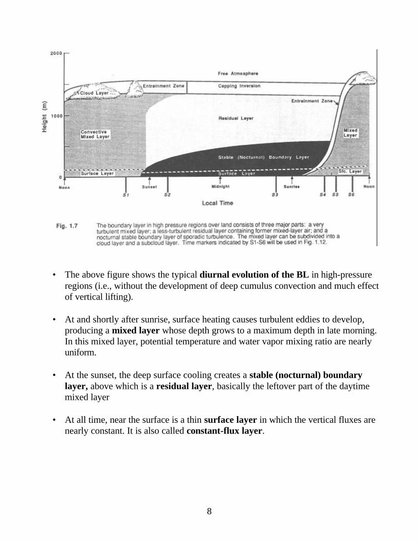
It is now safe to approximate ρ in (2.14) with ρ0 because the (first-order) effect of density perturbation on the buoyancy has been taken into account. The vertical equation with Boussinesq approximation is then

0 0

1 ' 'dw pg

dt zρ

ρ ρ∂

≈− −∂

(2.15).

(2.15) says that positive density perturbation (heavier air) creates negative buoyancy. Since with Boussinesq approximation, we assume the density is constant, the mass conservation equation is also simplified, from

1 d u v w

dt x y zρ

ρ ∂ ∂ ∂

= − + + ∂ ∂ ∂

to

0u v wx y z

∂ ∂ ∂+ +

∂ ∂ ∂; (2.16)

18

i.e., the flow is non-divergent. The thermodynamic energy equation is

d

Sdt θθ

= (2.17)

where Sθ represents heat source or sink and potential temperature θ is defined as

/

1000 pR Cmb

Tp

θ

=

(2.18).

It is easy to show (Holton p200) that

0 0 0

' 1 ' 'pp

θ ρθ γ ρ

≈ − (2.19)

where /p vC Cγ = is the ratio of the specific heat of dry air at constant pressure and constant volume. For typical atmospheric flows, the pressure perturbation part in (2.19) is much smaller than the density part, therefore

0 0

' 'θ ρθ ρ

≈ − (2.20)

With (2.20), we can replace density perturbation (which is not directly measured) by the potential temperature perturbation à

0 0

1 ' 'dw pg

dt zθ

ρ θ∂

≈− +∂

(2.21)

(2.21) says that positive potential temperature perturbation (warmer air) creates positive buoyancy, consistent with our physical understanding.

19

Equations (2.11), (2.16), (2.17) and (2.21) form a set of equations that we will use to derive the Reynolds averaged equations for describing the mean flow.

Reynolds averaged equations We divide all dependent variables in the above set of equations into the mean and perturbation parts. E.g., ' and 'u u u p p p= + = + . The terms on the right hand side of the equations are all linear in terms of these dependent variables, the mean of these terms will be equal to these terms of the mean variables only, i.e., the perturbation terms will drop out after the mean is taken. For example,

0 0

0 0 0

1 1 ( ')( ')

1 1 ' 1'

p p pfv f v v

x x

p p pf v f v f v

x x x

ρ ρ

ρ ρ ρ

∂ ∂ +− + = − + +

∂ ∂

∂ ∂ ∂= − + − + = − +

∂ ∂ ∂

(2.22)

because the mean of mean is equal to the mean itself and the mean of perturbation is zero. Therefore, as long as a term is linear, the mean of the entire time is equal to the term written for the mean variables. This is not true for nonlinear terms, such as the advection terms, however. Let's look at the left hand side of the u momentum equation, i.e., the du/dt term:

du u u u uu v w

dt t x y z

u uu vu wu u v wu

t x y z x y z

u uu vu wut x y z

∂ ∂ ∂ ∂= + + +

∂ ∂ ∂ ∂

∂ ∂ ∂ ∂ ∂ ∂ ∂= + + + − + + ∂ ∂ ∂ ∂ ∂ ∂ ∂

∂ ∂ ∂ ∂= + + +

∂ ∂ ∂ ∂

(2.23)

Chain rule of differentiation and zero divergence equations were used in the above.

20

Taking a Reynolds average of (2.23), we obtain

' ' ' ' ' '

' ' ' ' ' '

u uu vu wut x y z

u u u v u wu u u v u w ut x y z x y z

u u u u u u v u w uu v w

t x y z x y z

∂ ∂ ∂ ∂+ + +

∂ ∂ ∂ ∂

∂ ∂ ∂ ∂ ∂ ∂ ∂= + + + + + +

∂ ∂ ∂ ∂ ∂ ∂ ∂

∂ ∂ ∂ ∂ ∂ ∂ ∂= + + + + + +

∂ ∂ ∂ ∂ ∂ ∂ ∂

(2.24)

In the above, we again used the zero divergence condition for the mean velocity.

By defining d u u

u v wdt t x y z

∂ ∂ ∂ ∂= + + +

∂ ∂ ∂ ∂ which is the total time derivative

for the mean flow (equal to the local time derivative plus advection by the mean flow), the equations of motion become

0

1 ' ' ' ' ' 'd u p u u v u w uf v

dt x x y zρ ∂ ∂ ∂ ∂

= − + − + + ∂ ∂ ∂ ∂ , (2.25a)

0

1 ' ' ' ' ' 'd v p u v v v w vf u

dt y x y zρ ∂ ∂ ∂ ∂

= − − − + + ∂ ∂ ∂ ∂ , (2.25b)

0 0

1 ' ' ' ' ' ' 'd w p u w v w w wg

dt z x y zθ

ρ θ ∂ ∂ ∂ ∂

= − − − + + ∂ ∂ ∂ ∂ . (2.25c)

The thermodynamic energy equation (2.17) becomes

' ' ' ' ' 'd u v w

Sdt x y z θθ θ θ θ ∂ ∂ ∂

= − + + + ∂ ∂ ∂ . (2.25d)

21

The mass continuity equation for the mean flow is

0u v wx y z

∂ ∂ ∂+ + =

∂ ∂ ∂. (2.25e)

Similarly, when the Reynolds averaging is applied to the conservation equation of water vapor mixing ratio q, we obtain the Reynolds averaged equations for

' ' ' ' ' '

qdq u q v q w q

Sdt x y z

∂ ∂ ∂= − + + + ∂ ∂ ∂

(2.25f)

and the covariances in the square brackets are turbulent fluxes of water vapor.

2.2.3. Reynolds fluxes and their physical interpretation Equation set (2.25) is the Reynolds averaged equations for the mean state variables. The various covariances in the square brackets in the equations represent turbulent fluxes (a flux is always a quantity multiplied by a velocity). For example, ' 'w u is the vertical flux of momentum in the x direction or the flux of vertical velocity w in x direction. ' 'w θ is the vertical turbulent flux (flux due to turbulent motion) of heat. The heat flux is positive when w' and θ' are positively correlated, i.e., when w' and θ' tend to have the same sign. The end result is that warmer air gets transported by the turbulent velocity upward, and cold air gets transported downward, resulting in net positive (upward) heat flux. The net (turbulent) heat flux into a unit volume of air causes the temperature of this volume to change. This net flux is the difference between the flux going into a, for example, cubed volume on one side and that going out of the volume on the other side, it is therefore the flux divergence that causes

22

the change in the quantity being transported (by turbulence), which is θ in (2.25e) and q in (2.25f). For momentum, the flux of the momentum parallel to a volume face (e.g., the flux of u through lower boundary of a cubed volume by w) causes the parallel momentum (u in this case) to change at that face. Therefore the momentum flux is the stress (force /unit area) applied at this face. We therefore also call the momentum fluxes in the above momentum equations the Reynolds stresses. We often symbol τ is used to denote the stress. Let's look at the physical meaning of the fluxes in some more details. Let's look at the heat flux for example. Suppose we have an idealized turbulent eddies near the ground on a hot summer day. If we start with a particular profile of θ , how will it change with time? Due the surface heating, typically θ is super-adiabatic near the ground ( / 0d dzθ < ), as shown in the following figure. z z2 A z1 B θ Assume that we have two parcels, A and B. The A moves downward, and B upward. When A moves downward, it becomes colder than its environment, it therefore carries a negative θ'. For parcel B, it's the opposite, it carries a positive θ', therefore

23

For parcel A, w' < 0 and θ'< 0 à ' 'w θ > 0 therefore the heat flux is positive. For parcel B, w'>0 and θ' > 0 à ' 'w θ > 0 therefore the heat flux is also positive. Even though both fluxes are positive, the physical process is different – positive heat flux can be caused by either transporting (by turbulent eddies) colder air downward or transporting warmer air upward. Considering only the vertical turbulent heat flux (which tend to dominate in convective boundary layer), and assuming the mean velocity is zero (i.e., there is not mean wind advection) the heat energy equation (i.e., the equation for θ ) becomes

' 'w

t zθ θ∂ ∂

= −∂ ∂

. (2.26)

We see that temperature change as a result of heat flux divergence, not the heat flux itself. Temperature changes only when the net heat flux into an air parcel (or volume) is non-zero. In the above example, the flux at both level z1 and z2 are positive. But because the vertical gradient of θ is larger at z1, the flux there has a larger magnitude (this is a turbulence flux problem – one commonly used closure is to assume that the turbulent flux is proportional to the gradient of the mean quantity), therefore

2 1

2 1

( ' ') ( ' ')' '0z zw ww

t z z z

θ θθ θ −∂ ∂= − = − >

∂ ∂ −

therefore the mean potential temperature θ in the layer between z1 and z2 will increase with time! If the heat flux is positive at both level but increases with height, then the temperature will decrease in time (even though the heat flux is positive), because most heat is leaving this layer at the top boundary that the heat coming in from the bottom of this layer. Similar concept can be applied to turbulent fluxes of other material quantities such as water vapor mixing ratio, and to momentum.

24

2.3. PBL Equations for Mean Flow and Their Applications Read Holton Section 5.3!

2.3.1. The PBL Momentum Equations We have derived the Reynolds averaged equations in the previous section, and they describe the mean flow, taking into account the effect of turbulence motion. Generally, inside the boundary layer, vertical turbulent flux divergence is much bigger than horizontal one, because vertical shear/gradient is much bigger. We often consider the so-called horizontally homogeneous turbulence for which the horizontal turbulent flux divergence is neglected. We therefore have, from (2.25),

0

1 ' 'd u p w uf v

dt x zρ∂ ∂

= − + −∂ ∂

, (2.27a)

0

1 ' 'd v p w vf u

dt y zρ∂ ∂

= − − −∂ ∂

. (2.27b)

Consider further that the mean variables are for synoptic-scale horizontal flows, the acceleration terms are much smaller than the PGF and Coriolis terms, they can be neglected.

Further, because 0 0

1 1, andg g

p pfv fu

x yρ ρ∂ ∂

= = −∂ ∂

, we have

' '

( ) 0gw u

f v vz

∂− − =

∂, (2.28a)

' '( ) 0g

w vf u u

z∂

− − − =∂

. (2.28a)

They represent the balance among Coriolis force, pressure gradient force and the vertical momentum flux divergence (a net stress applied to the air parcel).

25

We will use the above two equations to solve for boundary-layer wind in two different models.

2.3.2. The Mixed Layer Model (Section 5.3.1 of Holton) As we saw earlier, in the well-mixed boundary layer, the mean wind and mean potential temperature are nearly constant with height. If we look at the flux profiles, they decrease linearly with height, and to zero at the top of boundary layer (they often go to negative values before becoming zero) where turbulence becomes weak. According to observations, the momentum fluxes at the surface can be accurately represented by the bulk aerodynamic formula (or drag law):

( ' ') | | ,

( ' ') | | ,

sfc d

sfc d

w u C V u

w v C V v

= −

= −

rr (2.29)

where Cd = non-dimensional drag coefficient and 2 2| |V u v= +r

is the wind speed at the surface, or more accurately at the anemometer height (10 m). The above formulae are very important and are used commonly in numerical weather prediction models to model the surface fluxes. Similar formulae are available for heat and moisture. The drag coefficient Cd depends on the roughness of the surface and the stability of the surface layer air. Over ocean, it is on the order of 10-3 and over land on the order of 10-2. Now that we know the fluxes at the surface (~z=0) and at the top of the boundary layer (z=h) and know that the fluxes are linear function of height. We also assuming that the mean wind is constant with height, we can easily integrate the above equations (2.28a,b), i.e.,

0 0

' '( )

h h

gw u

f v v dz dzz

∂− =

∂∫ ∫ à

26

0 0 0

' '( ) ' ' ' ' | |

h h

g dh

w uf v v dz dz w u w u C V u

z∂ − = = − = ∂∫ ∫

r à

( )

| |g

d

f v v hu

C V−

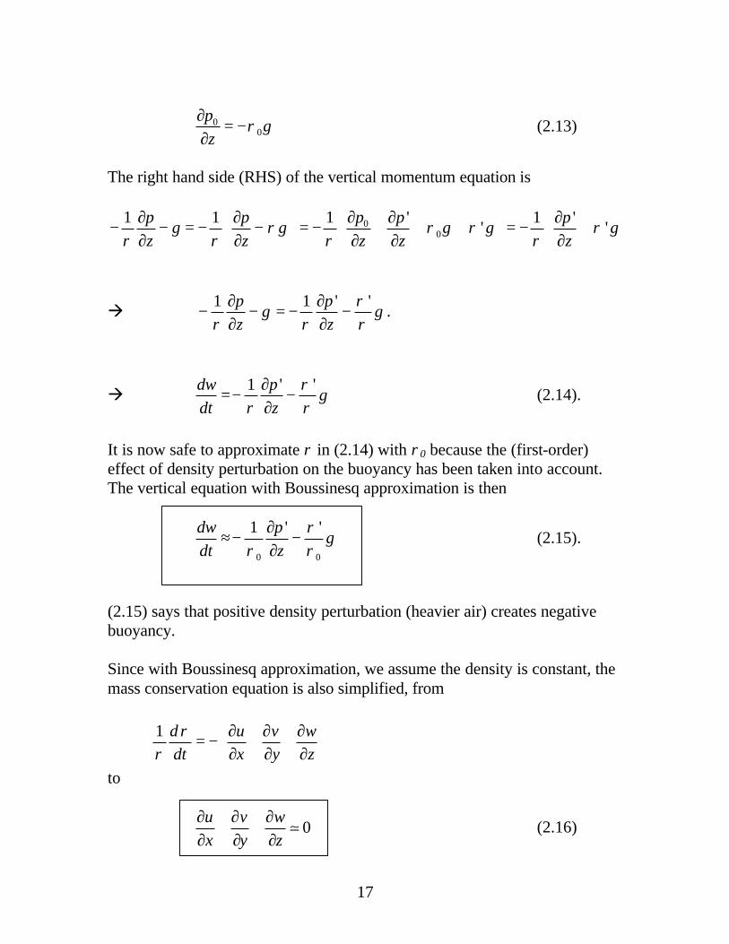
= r . (2.30a)

Similarly, ( )

| |g

d

f u u hv

C V

− −= r . (2.30b)

Without loss of generality, we can choose our coordinate system so that the x-axis is parallel to gu so that 0gv = . Therefore,

| |g su u K V v= −r

(2.31a)

| |sv K V=r

(2.31b)

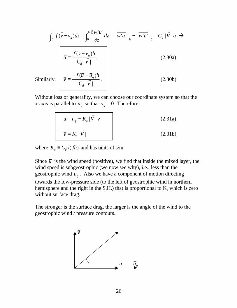
where /( )s dK C fh≡ and has units of s/m. Since u is the wind speed (positive), we find that inside the mixed layer, the wind speed is subgeostrophic (we now see why), i.e., less than the geostrophic wind gu . Also we have a component of motion directing towards the low-pressure side (to the left of geostrophic wind in northern hemisphere and the right in the S.H.) that is proportional to Ks which is zero without surface drag. The stronger is the surface drag, the larger is the angle of the wind to the geostrophic wind / pressure contours.

v u gu

27

Example, gu = 10 m/s Ks = 5×10-3 / (10-4 ×1000) = 0.05 s m-1 à u =8.28 m/s, v =3.77 m/s, | | 9.10m/sV =

r

at all height within this well mixed layer. All of this is consistent with what you have learned before about the three-force balance. In a geostrophic flow, the PGF and the Coriolis force are in balance. When friction is present, friction acts in the opposite direction as the velocity vector and is therefore also perpendicular to the Coriolis force. The balance between the three forces are illustrated as follows:

P-

PGFuuuuur

P0 φ V

r

rFr

Cor

uuuur

P+

As can be seen above, the wind vector is no longer parallel to the pressure contours, the flow is crossing the isobars to the lower pressure side! In vector form, the balance is expressed as

0

1ˆ | |dsfc

Cfk V p V V

hρ× = − ∇ −

r r r. (2.32)

The last term is sometimes called friction – but keep in mind that this is due to turbulent mixing, not molecular viscosity, the latter is much smaller.

28

2.3.3. K-Theory: First-order Turbulence Closure (section 5.3.2 of Holton) When the boundary layer is neutral or stable, the constant wind speed assumption used in the previous slab model is no longer good. To solve the equations for the mean variables, we have to express the turbulent fluxes in terms of the mean variables, to close the equation set (so that we have the same number of unknowns as the number of equations). This is called the closure problem. One of the commonly used methods is to express the fluxes in terms of the gradient of the mean variables, in a way analogous to the molecular diffusion. The flux is assumed to be proportional to the local gradient of the mean:

' ' ,mu

u w Kz

∂= −

∂ (2.33a)

' ' ,mv

v w Kz

∂= −

∂ (2.33b)

and similarly to the potential temperature:

' ' hw Kzθ

θ∂

= −∂

. (2.33c)

We call Km the eddy viscosity (has units of m2/s) and Kh the eddy diffusivity of heat. This closure scheme is often called the K-theory. With the closure given in (2.33), we can write equations in (2.27) as

0

1m

d u p uf v K

dt x z zρ∂ ∂ ∂ = − + + ∂ ∂ ∂

, (2.34a)

0

1m

d v p vf u K

dt y z zρ∂ ∂ ∂ = − − + ∂ ∂ ∂

. (2.34b)

29

We see that the perturbation variables no longer appear in the equations. Given p we can solve for andu v . For the potential temperature, the equation is

hd

K Qdt z z θθ θ ∂ ∂

= + ∂ ∂ . (2.34c)

We will use this set of equations to obtain the Ekman layer solution in the next section. Note also that the K-theory actually has a number of limitations.

• Firstly K should be flow-dependent and it is often not easy to determine its value.

• Secondly, often the eddies that cause most of the mixing have sizes

that are comparable to the PBL depth and are therefore not so much related to local gradient therefore the closure assumption does not work well. For this reason, certain non-local closure schemes have been developed.

2.3.4. The Ekman Layer (Section 5.3.4 of Holton) The Ekman layer is the part of the atmosphere that extends from the anemometer level up to the height where the gradient wind balance holds (PGF + COR + CENTRIF). In this layer, we make the following assumptions within the context of K-theory:

a) The force balance is among PGF, Coriolis and turbulence. Centrifugal force is neglected.

b) The flow is steady-state, i.e., / 0t∂ ∂ = . c) The atmosphere is horizontally homogeneous, i.e., ( ) / ( ) / 0x y∂ ∂ + ∂ ∂ = .

this implies that gVr

is independent of height, via the thermal wind law. d) Lapse rate is neutral, i.e., / 0zθ∂ ∂ = . So, the PBL is well mixed. e) Km is constant f) Earth is flat with w =0 at ground. g) Flow is incompressible.

30

With these assumptions, our mean flow momentum equations in (2.34) become

2

2 ( ) 0m gu

K f v vz

∂+ − =

∂ (2.35a)

2

2 ( ) 0m gv

K f u uz

∂− − =

∂ (2.35b)

The above two equations are coupled. One way to simplify the solution procedure is to combine the two equations into one, by using complex variables. Define complex velocities w u iv= + and g g gw u iv= + . (2.35a) + i (2.35b) à

2

2

( )( ) 0m g g

u ivK f v ui v u i

z∂ +

+ − − + =∂

à

2

2

( )( ) 0m g g

u ivK fi iv u iv u

z∂ +

+ − − + + =∂

à

2

2 ( ) 0m gw

K fi w wz

∂− − =

∂ (2.36)

Since we assumed that gw is constant with height, (2.36) can be rewritten as

2

2

( )( ) 0g

gm

w w i fw w

z K

∂ −− − =

∂ (2.37)

which is a linear, 2nd-order ODE for ( )gw w− with constant coefficients – a basic ODE problem. The characteristic equation for (2.37) is

2 0m

i fK

λ − =

31

therefore m

i fK

λ = ± there λ's are the eigenvalues of the PDE. The solutions

to (2.37) are therefore (verify for yourself):

m m

i f i fz z

K Kgw w Ae Be

−

− = + . (2.38) Here A and B are arbitrary constants to be determined by the boundary conditions. The boundary conditions are w =0 at z = 0 à 0 gw A B− = +

asgw w z= → ∞ à 0 m

i fz

KAe= à A = 0. Therefore gB w= − . Solution (2.38) becomes

m

i fz

Kg gw w w e

−

= − Without loss of generality, we choose our x coordinate axis to be parallel to the geostrophic wind, so that wg = ug, vg=0.

m

i fz

Kg gw u u e

−

= − (2.39) Let's see what i is equal to. 2 21, 1 1 1, (1 ) (1 1)i i i= − + = + − + = + −

2 1(1 ) 1 2 1 1 2

2i

i i i+

+ = + − − = → =

Our solution is therefore

32

(1 )

2(1 )m

fi z

Kgw u e

− +

= − à [1 cos( ) sin( )]z z

gu iv u e z ie zγ γγ γ− −+ = − + à [1 cos( )]z

gu u e zγ γ−= − (2.40a)

sin( )zgv u e zγ γ−= (2.40b)

When plotted the solution on a hodograph, which is a plot of the wind vector on a polar coordinate diagram, we obtain what is called the Ekman Spiral solution as shown below:

We see that with this solution, there is an ageostrophic wind component pointing to the left of geostrophic wind, i.e., towards the low-pressure side, this agrees with the results of the earlier mixed-layer model, and the solution represents a three-way balance, i.e., a balance between the PGF, Coriolis and frictional forces. The idealized Ekman spiral wind profile is rarely observed in the atmosphere, however, because of other effects that are not considered in the idealized model. In the surface layer, the equations used to obtain this solution are not valid. One way to take it into account is to match the Ekman

33

layer solution with that in the surface layer, doing so gives us the so called modified Ekman layer solution is that often a better match of the observations. The following figure gives such an example.

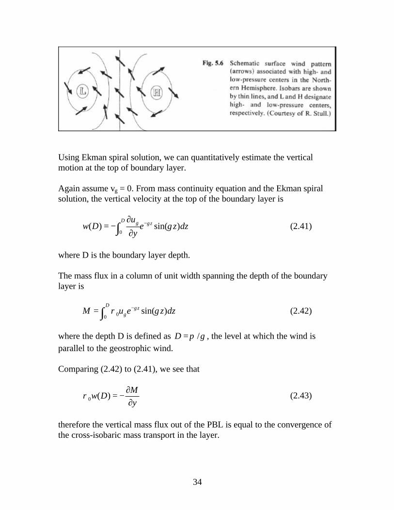
2.3.5. Secondary Circulation and Spin-Down (Section 5.4 of Holton) From both the Ekman layer solution and the mix-layer solution obtained in section 2.3.2 (Equation 2.31), we know that the friction reduces the boundary layer wind speed below geostrophic wind, and causes it to cross the isobars from high towards low pressure. In a synoptic situation where the isobars are curved, such as a low or high pressure systems, the cross-isobaric component of flow near the surface causes rising air in low-pressure systems and descending air in highs. The processing of inducing vertical motions by boundary layer friction is call Ekman pumping.

34

Using Ekman spiral solution, we can quantitatively estimate the vertical motion at the top of boundary layer. Again assume vg = 0. From mass continuity equation and the Ekman spiral solution, the vertical velocity at the top of the boundary layer is

0

( ) sin( )D g zu

w D e z dzy

γ γ−∂= −

∂∫ (2.41)

where D is the boundary layer depth. The mass flux in a column of unit width spanning the depth of the boundary layer is

00sin( )

D zgM u e z dzγρ γ−= ∫ (2.42)

where the depth D is defined as /D π γ= , the level at which the wind is parallel to the geostrophic wind. Comparing (2.42) to (2.41), we see that

0 ( )M

w Dy

ρ∂

= −∂

(2.43)

therefore the vertical mass flux out of the PBL is equal to the convergence of the cross-isobaric mass transport in the layer.

35

Further, gg

u

yξ

∂=

∂, the geostrophic vorticity, and substituting the Ekman

spiral solution into (2.41), we obtain

1 / 2

( )2 | |

mg

K fw D

f fξ

=

(2.44)

hence the vertical mass flux is proportional to the geostrophic vorticity and the square root of the boundary layer eddy viscocity. In the northern hemisphere, w at Z=D is positive inside a cyclone ( 0)gξ > and negative inside an anticyclone. This w induces a secondary (vertical) circulation as shown below. Above the PBL inside a cyclone, there exists divergence, according to angular momentum conservation, the horizontal rotation rate (vorticity) will decrease with time, hence the spindown of the cyclone. A quantitative discussion of this using a vorticity equation is given in Holton section 5.4. Read it yourself!

36

Tea Cup Example. After the tea in a cup is stirred, the bottom friction slows down the spinning tea in the cup near the bottom surface, breaking the balance between the PGF and centrifugal force. The PGF cause the secondary circulation/flow towards the center of the cup near the bottom and induces compensating flow above this layer away from the central axis. To conserve angular momentum, the spin has to slow down. This is analogous to the spindown of a cyclone.

37

2.4. Applications of Boundary Layer Meteorology

2.4.1. Low-level Jet See Dr. Keith Brewster's Notes

2.4.2. Temporal Evolution & Prediction of the PBL Earlier, we saw the following figure showing the diurnal evolution of PBL.

With a typical diurnal cycle, the PBL (well-mixed layer in particular) grows by a 4-phse process:

1) Formation of a shallow M.L. (burning off of the nocturnal inversion), ~ 10's to 100's meter deep

2) Rapid ML growth, surface thermals rises easily to the to of residual layer

3) Deep ML of nearly constant thickness. Growth slows down with the present of capping inversion. Entrainment roughly balances the

38

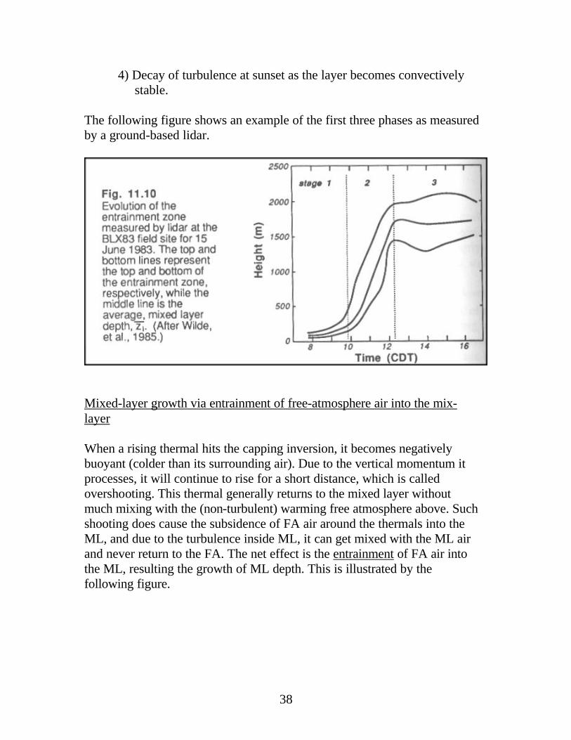
4) Decay of turbulence at sunset as the layer becomes convectively stable.

The following figure shows an example of the first three phases as measured by a ground-based lidar.

Mixed-layer growth via entrainment of free-atmosphere air into the mix-layer When a rising thermal hits the capping inversion, it becomes negatively buoyant (colder than its surrounding air). Due to the vertical momentum it processes, it will continue to rise for a short distance, which is called overshooting. This thermal generally returns to the mixed layer without much mixing with the (non-turbulent) warming free atmosphere above. Such shooting does cause the subsidence of FA air around the thermals into the ML, and due to the turbulence inside ML, it can get mixed with the ML air and never return to the FA. The net effect is the entrainment of FA air into the ML, resulting the growth of ML depth. This is illustrated by the following figure.

39

Thermodynamic ML Growth Model We can predict the depth of the ML using a simple method called the Thermodynamic Method – it focuses only on the thermodynamic process and neglects the dynamics of turbulent entrainment. The method actually has a nice physical basis. Consider an early morning sounding of θ as shown in the following figure.

40

If later in the morning (at time t1), the temperature reaches θ1 due to surface heating, then the mixed layer depth is z1. The amount of energy (heat) needed to reach this state is shaded and has a dimension of MK (mass times degree). Note that more heat is required to reach a deeper M.L. The total heat required should be equal to the total heat flux from the surface for the period proceeding time t1. In the time-flux diagram, it is equal to the shaded area below the heat flux curve between time t0 and t1. To estimate the ML depth at t=t1, we need to

1) Find the area under the hear flux curve upto time t1 (assuming the heat fluxes can be estimated, this is the job of a land surface model in a NWP model),

2) Estimate which adiabat in the early AM sounding corresponds to that amount of heat

3) ML depth = height where that adiabat intercepts with AM sounding Note that this method neglects advection and direct radiation effects and the effect of vertical motion (subsidence or ascend). We can do this mathematically using our energy equation:

( ' ')w

t zθ θ∂ ∂

= −∂ ∂

.

Now, integrate over height and time:

1 1 1 1 1 1

10 0 0 0

0 00 0

( ' ')[( ' ') ( ' ') ] ( ' ')

z t z t t t

zt t t t

wdtdz dtdz w w dt w dt

t zθ θ

θ θ θ∂ ∂

= − = − − =∂ ∂∫ ∫ ∫ ∫ ∫ ∫

The left hand side of the equation is

1 1 1 1 1

0 01 00 0 0

( )z t z z

tdtdz d dz dz

t

θ

θ

θθ θ θ

∂= = −

∂∫ ∫ ∫ ∫ ∫

which we see easily from the above figure is the shaded area to the right of the θ curve and the left of the adiabat at t1. This area is also equal to

41

1

0

( )z dθ

θθ θ∫ .

Therefore, we can estimate the total heat surface heat flux until certain time, we can predict the depth of the ML at that time. This is important to thunderstorm prediction before the maximum depth of the ML can grow to has an important implication as to if an inversion cap can be broken or not and if free convection can occur.

2.4.3. Development and Evolution of Drylines The dryline is another mesoscale phenomena whose development and evaluation is strongly linked to the PBL. Text books containing sections on dryline: The Dry Line. Chapter 23, Ray, P. S. (Editor), 1986: Mesoscale Meteorology and Forecasting. American Meteorological Soc., 793 pp.. Pages 292 – 290. Bluestein, H. B., 1993: Synoptic-Dynamic Meteorology in Midlatitudes. Vol. 2: Observations and Theory of Weather Systems. Oxford University Press, 594pp. The dryline 1. Definition: A narrow zone of strong horizontal moisture gradient at and

near the surface. 2. Observed in the Western Great Plains of the U.S. (also in India, China,

Australia, Central Africa,....) 3. Over the U.S., the dry line is a boundary between warm, moist air from

the Gulf of Mexico, and hot, dry continental air from the southwestern states or the Mexican plateau

42

In this example, some 200C dew-point temperature gradient is observed

across the dryline in the above example. 4. The dry line is not a front; i.e., there is very little density contrast

between warm, moist air and hot, dry air (because dry air is more dense than moist air – the two effects offset each other – virtual temperature – a measure of relative-density of moist air, is (1 0.61 )vT T q= + )

5. A veering wind shift usually occurs with dry line passage during the day

because the dry adiabatic lapse rate behind the dry line facilitates vertical mixing of upper-level westerly momentum down to the surface.

0.6C 19.4C

43

6. The dry line is often located near a surface pressure trough (often a lee

trough or "heat trough"), but does not have to be coincident with the trough. (see the first example).

7. Typical moisture (in terms of dew-point temperature) gradient is 150C

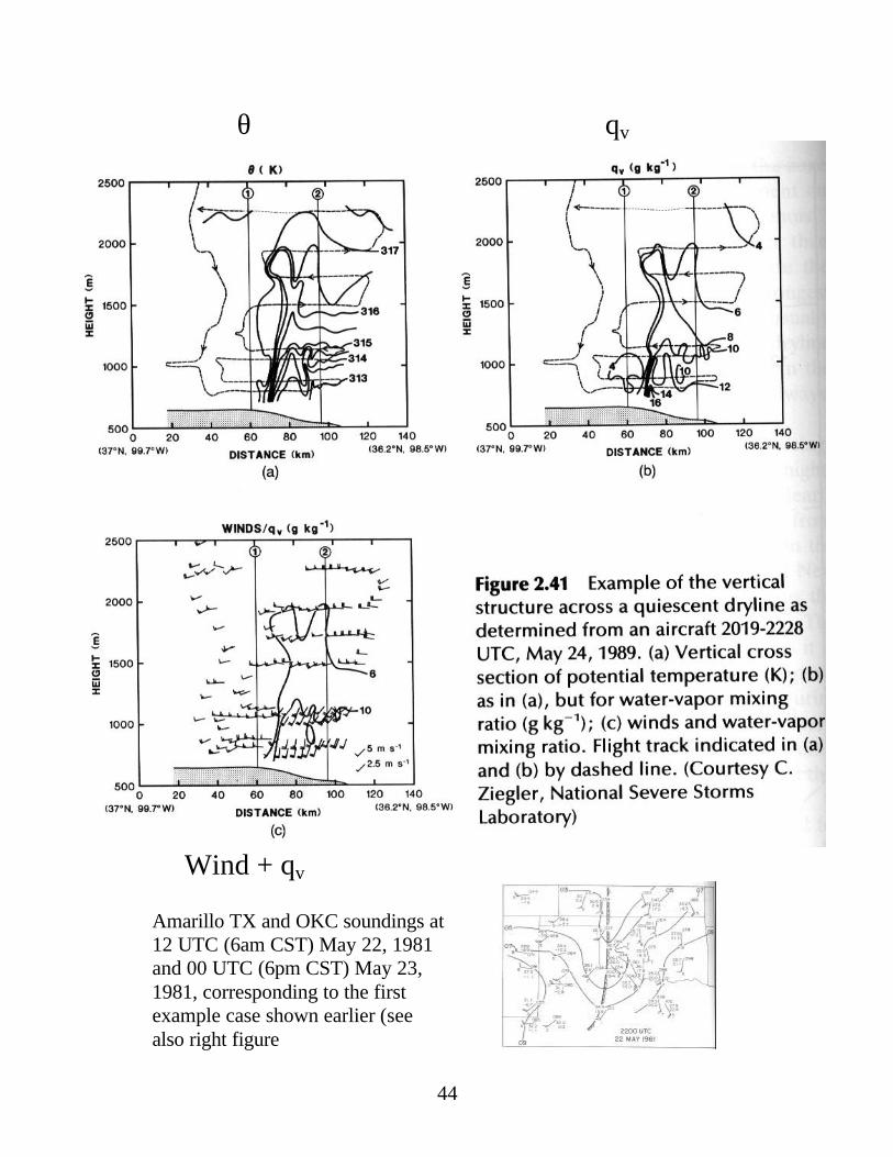
per 100 km, but 90C in 1 km has been observed. 8. Vertical structure: Is nearly vertical for < 1 km and then "tilts" to the east

over the moist air (see Figures)

44

θ qv

Wind + qv

Amarillo TX and OKC soundings at 12 UTC (6am CST) May 22, 1981 and 00 UTC (6pm CST) May 23, 1981, corresponding to the first example case shown earlier (see also right figure

45

46

The May 11, 1970 Case

Dryline was between Carlsbad, N. Mexico (Td = 25 F) and Wink, TX (Td = 57 F).

• Strong moisture gradient is found across the dryline

• Nocturnal inversion is found at the surface.

• An inversion is found to the east of the dryline at ~850mb level, capping moist air below

• No clear horizontal θ gradient separating the dry and moist air

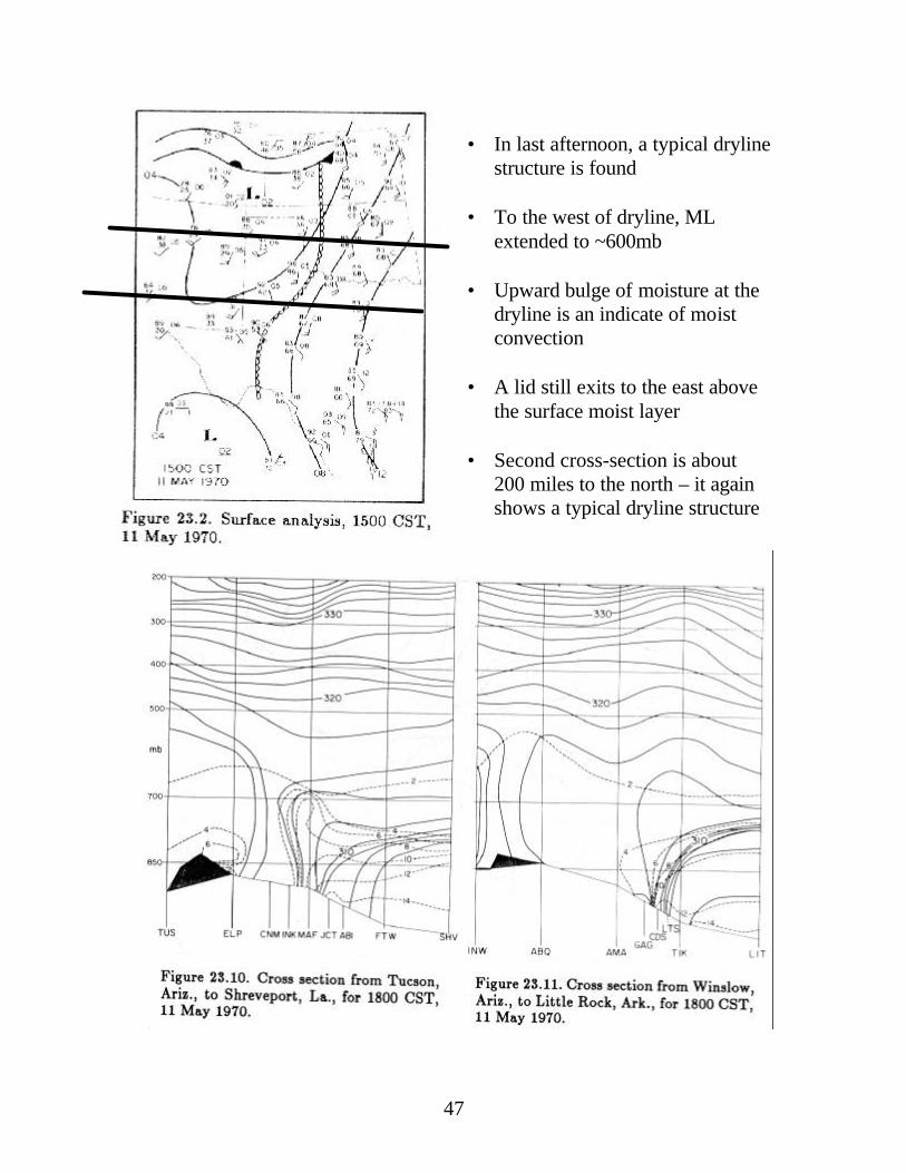
47

• In last afternoon, a typical dryline

structure is found

• To the west of dryline, ML extended to ~600mb

• Upward bulge of moisture at the dryline is an indicate of moist convection

• A lid still exits to the east above the surface moist layer

• Second cross-section is about 200 miles to the north – it again shows a typical dryline structure

48

TYPICAL BACKGROUND CONDITIONS FOR THE FORMATION OF THE DRY LINE

1. Surface anticyclone to the east, allowing moist Gulf air to flow into the Great Plains

2. Westerly flow aloft, causing a lee trough, and providing a confluence

zone for the concentration of the moisture gradient 3. The presence of a stable layer or "capping inversion" or "lid" aloft. The

southerly flow under this lid is often called "underrunning". 4. Because the terrain slopes upward to the west, the moist layer is shallow

at the west edge of the moist air, and deeper to the east.

This sets the stage for understanding the movement of the dry line. MOVEMENT OF THE DRY LINE Under "quiescent" (i.e., in the absence of strong synoptic-scale forcing) conditions, the dryline usually moves eastward during the day and westward at night, as shown by the following example (we have just looked at the vertical structure of this case)

49

50

1. As the sun rises, the heating of the surface near the dry line is greater than

that of the surface to the east in the deeper moist air (the difference in soil moisture content and low-level cloudiness often also contribute to such differential heating)

2. Thus it takes less insolation to mix out the shallow mixed layer just to the

east of the initial dry line position (see Figure). This mixing out brings dry air (and westerly momentum) downward, and the position of the dry line moves eastward.

3. As the heating continues, deeper and deeper moist layers are mixed out, causing the apparent eastward "propagation" of the dry line. This propagation is not necessarily continuous or at a rate equal to the wind component normal to the dry line.

51

4. Eventually, the heating is insufficient to mix out the moist layer and

propagation stops. 5. If a well-defined jet streak exists aloft, we often see a "dry line bulge"

underneath the jet, as this air has the most westerly momentum to mix downward. The strong westerly momentum mixed down from above provides extra push for the eastward propagation of dryline

6. After sunset, the vertical mixing dies out, the dry line may move

westward back toward the lee-side pressure trough,

As vertical mixing ceases, the surface winds will back to a southeasterly direction in response to the lower pressure to the west. The moist air east of the dry line will be advected back toward the west, and surface stations will experience an east to west dry line passage.

52

The above case assuming synoptic scale forcing is weak – the situation is quiescent. If synoptic forcing is strong, the dryline may continue to be advected eastward in association with a surface low pressure system.

53

Often, a cold front will eventually catch up to the dry line.

54

The dryline as a focus of convection Possible reasons why convection initiates near dry lines:

1. Surface convergence between winds with easterly component east of the

dry line and westerly component west of the dry line. 2. General region for large-scale forcing aloft if short-wave is moving over

the Rockies and out into the Plains. 3. Gravity waves may form on or near the dry line, possibly triggering the

first release of potential instability. 4. Dryline bulges provide an even greater focus for surface moisture

convergence 5. "Underrunning" air moves northward until cap is weaker and/or large- or

mesoscale forcing is strong enough to release the instability (see April 10, 1979 figures)

6. The upper-level cloud edge may be east of the surface dry line, allowing

surface heating to occur while strong forcing for upward motion exists aloft (the northern end of a dry slot). This combined destabilization may produce "dryslot convection" (Carr and Millard, 1985)

7. Convective temperature may be reached just east of the dry line.

Some observations: The reason for most tornado chase "busts" is that the advection of warm, dry air over the moist layer is building the cap or lid strength faster than the surface heating can overcome, thus convection never occurs.