Embed Size (px)
Citation preview
38
CHAPTER 2 - STUDY AREA
2.1. GENERAL BACKGROUND OF THE STUDY AREA
2.1.1. Oceanographic studies in North-western Indian Ocean
(Arabian Sea)
2.1.2. Historical Background
The origins of “ocean science” in the north-western Indian Ocean, also
generally known as the Arabian Sea, extend back to ca. 2,300 B.C., when trade
between the Mesopotamian peoples in the Persian Gulf and those of the Indus
Valley was established, and trade between Egypt and Somalia (then called Punt)
was similarly underway (Warren, 1987). The regularly reversing surface current
was not correctly described until A.D. 912, when the traveller El Mas’u’di’
crossed the “sea of the Zanj” as the western Arabian Sea was then known, and
described the nature of the Sea, such as the waves, dangers, monsoon winds and
currents (Warren, 1987).
Ocean Science came to fruition through the CHALLENGER Expedition
of 1873-1876. The expedition greatly expanded man's knowledge of the world's
oceans and revolutionized the ideas about planet Earth. However, the Challenger
expedition did not survey in the Arabian Sea. The first major oceanographic
investigation there, was carried out during 1933-34, on the John Murray
MABAHISS Expedition. Exploration increased rapidly in the period 1959-1965,
during the course of the International Indian Ocean Expedition (IIOE), with the
participation of thirteen nations and at least forty ships. The Geochemical Ocean

39
Sections Study (GEOSECS) made a survey of the Indian Ocean in 1977-78
covering the Arabian Sea, the Bay of Bengal and the south Indian Antarctic
Ocean. The GEOSECS Indian Ocean data are summarized in a compilation of
data (Weiss et al. 1983) and in an atlas (Spencer et al. 1982). During the last three
decades, comprehensive studies of the physical, chemical and biological
oceanography have also emerged as a result of major surveys carried out by
Indian Scientists. The investigations have been made during the cruises of the
Indian Naval Ships (INS) DARSHAK (1973-74) and R.V. GAVESHANI during
1976 and O.R.V. SAGAR KANYA in the northern Arabian Sea. Recently, other
countries have also undertaken expeditions in the Arabian Sea.
Despite this intensive interest, a number of questions remain unanswered.
For example, it is not yet clear whether the north-western Indian Ocean (Arabian
Sea) is a sink for atmospheric carbon dioxide, due to high rates of primary
productivity and burial of sedimentary carbon, or a source via outgassing of
carbon dioxide to the atmosphere during upwelling. These processes affect the
carbon balance and the global carbon cycle. Furthermore, the Arabian Sea
exhibits extremes in atmospheric forcing that lead to the greatest seasonal
variability observed in any ocean basin. The wide range of climatic variability in
the Arabian Sea, makes it possibly the best place in the present-day ocean to look
clearly at past climates and possible future climatic change.
The Arabian Sea has other features which augment monsoonal forcing,
thus compelling the basin as attractive site for study. In the north, there is no
outlet, but the basin’s waters and sediments are influenced by inflow from the
Persian Gulf and the Red Sea, and by exchange across the equator. In the
following sections, the characteristics of the Arabian Sea are reviewed in detail.

40
2.2. Setting of the Arabian Sea
The Indian Ocean is surrounded by an asymmetrical distribution of
landmasses characterized by markedly different geology. Although details of
their geology are complex, the major shield areas, which surround the ocean
basin, namely Africa-Arabia, India, Australia, and Antarctica were formed after
the breakup of Gondwana land.
The main physiographic features of the Indian Ocean north of the Equator
is shown in Fig.2.1(A, B & C). The Arabian Sea, the area of this study, is
bordered by Arabia in the west, Iran and Pakistan to the north and India and the
Chagos-Laccadive ridge to the east. The Arabian Sea occupies the total area of
about 6.2 x 10⁶ km2 between 00 and 250 N and 500 and 800 E. The Persian Gulf
connects the Arabian Sea through the Gulf of Oman by a 50 m deep sill at the
Hormuz Strait. Similarly, the Red Sea is separated from the Arabian Sea through the
Gulf of Aden by a 125 m deep sill at the strait of Bab-el-Mandab. The Arabian Sea
receives its fluvial input primarily from the Indus River, which drains the
Himalayas as well as a large area of semi-arid to arid land in West Pakistan and
Northwest India, transporting over 400 million tons of suspended sediments a year.
A number of small rivers, chiefly the Narbada, with a common outlet to the
Arabian Sea through the Gulf of Cambay, drain the middle portion of India where
the soils derive from the weathering of the Deccan Traps. The Narmada and Tapti
rivers in India are the only other rivers of significance. The Arabian Basin itself is
separated from the Somali Basin by the Carlsberg Ridge, which reduces the flow of
bottom water into the Arabian Basin.
41
2.2.1. Continental Margin
The continental slope and shelf are wider on the Indian than the Arabian side
of the Arabian Sea, therefore exposing a larger area of the sea floor to the oxygen-
poor water. Much of the Oman margin is characterized by a narrow continental
shelf, bordered by an extremely steep continental formation of the margin
(Whitmarsh, 1979; Stein and Cochran, 1985). The continental margin beneath the
upwelling zone is a complex mixture of wide and narrow shelves, upper slope
basins and ridges, and submarine canyons (Prell et al. 1990; Mountain and Prell,
1989, 1990).
The tectonism of the Oman margin has resulted in the formation of the
Owen Ridge and Murray Ridge which separate the Owen Basin from the deep
abyssal plain and submarine fan of Indus cone. The Oman basin is roughly
triangular in outline and occupies the central floor of the Gulf of Oman at a depth
of about 3000 m. The Arabian basin has a maximum depth of 4500 m and merges
to the north into the Indus cone.

43
The Owen Ridge is an asymmetric, north-east-trending ridge that
originates at about 150 30’N, 59050’E, where the Sharbithat Ridge intersects the
Owen Fracture Zone, and extends to about 200 N, 610E, where it merges with the
Murray Ridge. The trend of the Owen Ridge is somewhat oblique to the Arabian
continental margin and its distance from land is about 320 km in the south and
about 200 km in the north. The Owen basin, which lies between the Arabian
margin and the Owen Ridge, is sediment filled and has depths of 3200-3500 m.
The Owen Ridge lies about 350 to 400 km off the Oman coast and is
within their territorial waters. The continental shelf off Oman is characterized by
broad wide segments, such as off Sequira, separated by narrow shelves that
merge with headland projections, such as off Ras el Madraka. The upper slope of
the margin is characterized by several basins that are sub-parallel to the shelf
break. These narrow basins lie as shallow as 400 m and as deep as 1,000-1,500 m
and result in a step-like margin (Mountain and Prell, 1989, 1990).
2.3. Climatic forcing of the Arabian Sea - the Monsoons
The term ‘monsoon’ is derived from the Arabic word ‘mausim’ which
refers to the seasonal reversal of winds around the Arabian Sea (Warren, 1966).
The Southwest Indian Monsoon system is one of the most important climatic
features of the world, impacting most of Africa, southern Asia and the Indonesian
archipelago. The success or failure of the monsoon rains in southern Asia and
northern Africa affects every phase of life (Prell et al. 1992).

45
2.3.1. Monsoon Systems
Schott et al. (1990) defined the monsoon periods, namely southwest
monsoon (June-September inclusive), north-east monsoon (December-February
inclusive), autumnal transition (October-November inclusive), and spring
transition (March-April inclusive). Only May does not fit into one of the four
major monsoonal seasons of the Arabian Sea.
2.4. Physical Oceanography
The climate and hydrography of the Northern Indian Ocean are mainly
controlled by the monsoonal circulation. The northern Indian Ocean is different
from other major oceans, because of a reversal of the atmospheric and surface
oceanic circulations. The major circulation systems in the Indian Ocean can be
described (Wyrtki, 1973) in three distinct categories namely:
1) Seasonally changing monsoonal gyre
2) The Southern hemispheric tropical gyre
3) The Antarctic waters with circumpolar current
The latter two systems are essentially similar to those of other oceans,
whereas the reversing monsoonal gyre is unique to the Indian Ocean. The
monsoonal circulation is a direct consequence of the changing wind patterns and
the closure of the ocean to the north by the large Asian continent. The monsoon
winds are the dominating factor in controlling the surface currents in the Arabian
Sea (Fig. 2.3). The currents are stronger during the southwest monsoon; wind
changes to the southwest in the summer. The flow in the intermediate layers is not

46
well known, although it seems that it may also be affected by the monsoonal wind
changes (Wyrtki, 1971). The winds are predominantly from the north-east during the
winter, and the water circulation is cyclonic (counter clockwise).
2.4.1. Water Masses
The deep and bottom water mass circulations, important to near-bottom
sedimentary processes and the major transport pathways of the high-salinity
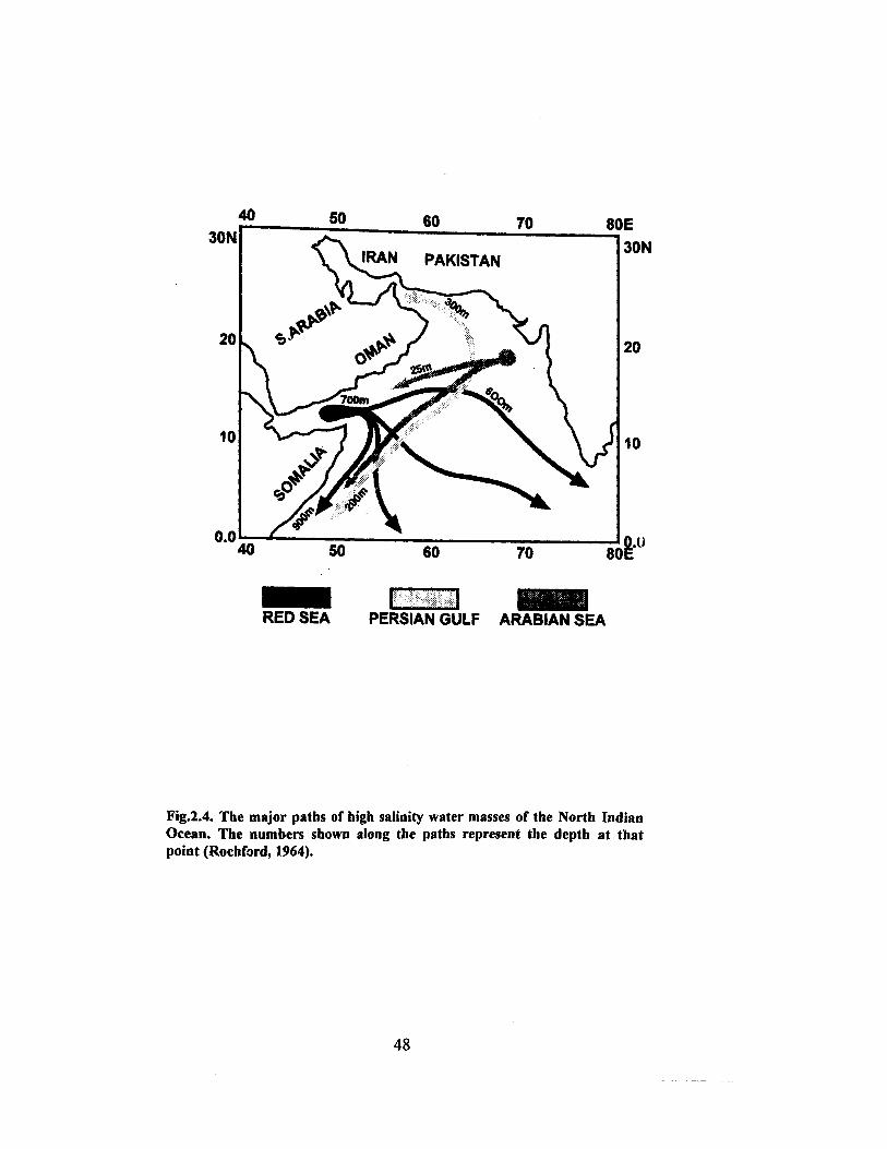
water indicating with corresponding depths are shown in Fig. 2.4. Deep water
masses are characterized by their density, temperature, salinity and oxygen
content. The water masses in the Indian Ocean are:
1. North Indian high-salinity intermediate waters (25-100 m)
2. Antarctic intermediate water (2000-2500 m)
3. Antarctic bottom water/Atlantic deep water (2500-3500 m).

49
2.4.2. Oman Upwelling System
The monsoonal upwelling system of the Arabian Sea reaches its acme
during summer months (Wyrtki, 1971; Krey and Babenerd, 1976; Prell and
Streeter, 1982), resulting in high productivity. The strong winds blow from the
south-west in summer (rainy season), and from the north-east in the winter (dry
season), causing a reversal of the surface circulation from clockwise to anti-
clockwise (Wyrtki, 1971). Monsoonal upwelling occurs along the coasts of
Arabia and Somalia (Bruce, 1974; Currie et al. 1973) and also locally along the
west coast of India (Sharma, 1976, 1978). During the southwest monsoonal
season, strong offshore Ekman transport of surface waters, leads to their
replacement by colder, nutrient-rich waters from several hundred metres deep
(Currie et al. 1973). The wind speed and the duration of the monsoon control the
strength and duration of the upwelling, which in turn causes controls enhanced
production of biogenic sedimentary components. By identifying the processes
that control the production and preservation of various sedimentary components,
the clastic and biogenic components deposited beneath the centres of upwelling
can be used to interpret the history of monsoonal upwelling, including upwelling
intensity, monsoon strength, and the oceanographic history of surface waters in
the northwest Arabian Sea.
50
2.5. Chemical Oceanography
2.5.1. Salinity
The Arabian Sea has high surface salinity ranges from about 36.2 to above
36.5 due to evaporation. The intermediate waters of the north-west Arabian Sea
(200-1000 m of water depth) known as North Indian Intermediate waters (NIIW)
are characterized by high salinity (34.8; Wyrtki, 1971, 1973) and by spatial and
temporal stability. The Red Sea and the Persian Gulf overflows, which spread at
about 800 m and 300 m, respectively, are the sources for the intermediate waters
(Swallow, 1984).
2.5.2. Nutrients
During SW Monsoon periods, the nutrient concentrations are higher in
surface coastal waters off both Somalia and Arabia (Wyrtki, 1971; Qasim, 1982).
In the offshore regions the concentrations are lower indicating more consumption
with higher productivity during the SW Monsoon periods (Reddy and
Sankaranarayanan, 1968). The levels of nutrient are inversely correlated to
dissolved oxygen due to organic matter degradation (Ryther et al. 1966).

51
2.6. Primary Production
The Arabian Sea is an area of high productivity averaging about twice
that of the world oceans (Ryther et al. 1966), and productivity is unique in its
magnitude among all oceans of the Northern hemisphere at these latitudes (Yoder
et al. 1991). High productivities are especially apparent in the north-western
sector (Qasim, 1977; Sen Gupta and Naqvi, 1984) due to the very high nutrient
concentrations. In response to richer nutrient supplies, the annual rates of primary
production in the northern Arabian Sea averages >500 mg C/m2/day in May to
October, dropping to values as low as 150 mg C/m2/day during November to
April (Krey and Babenerd, 1976, Qasim, 1982). Daily rates can exceed 2 g C m-2
d-1 (Qasim, 1982), reaching perhaps 6 g C m-2 d-1 (Babenerd and Krey, 1974).
The unusual atmospheric forcing of the region also creates areas of high primary
productivity that are adjacent to areas of perennially low primary production.
2.6.1. Plankton Patterns
The sediments are characterized by a variety of fossil plankton (both
phytoplankton and zooplankton) that are associated with active upwelling and its
productivity (Prell, 1984; Cullen and Prell, 1984; Kroon, 1988). For example the
foraminiferan species, Globigerina bulloides, seems to be associated with tropical
upwelling systems. Outside sub-polar waters, G. bulloides is abundant only in the
western Arabian Sea and the Cariaco Basin in the Caribbean, which is also a
seasonal upwelling system (Peterson et al. 1991). G. bulloides exhibits distinct
abundance gradients and constitutes more than 40% of all of the planktonic

52
foraminifera preserved in the sediments along the coast of Oman and decreases
seaward (Prell et al. 1992). The distribution of G. bulloides in the sediments and
its relation to seasonal temperature and chemical indices of upwelling, indicates
that its abundance is linked to the highly productive periods of the southwest
monsoon. High rates of foraminiferan flux during the south-west monsoon season
are predicted from the sediment record and sediment trap data.
2.7. Oxygen Minimum Zone
An important characteristic of upwelling areas is the oxygen minimum
zone (OMZ) that lies below the source waters of the upwelling system (Margalef
and Estrada, 1981). A water mass representing an oxygen minimum layer is
present (Fig.2.4A) between ~ 200-1200 m.b.s in the northern Indian Ocean,
including the Arabian Sea and Bay of Bengal. The stable zone of oxygen
depletion, the OMZ, is produced by the combined effect of restricted horizontal
advection of central Indian Ocean water, such as the Persian Gulf, Red Sea, and
Banda Sea waters, which are relatively impoverished in oxygen, stable salinity
and temperature stratification, and high chemical oxygen demand due to
upwelling-related high productivity (>500 mg C/m2/day). These lead to the
development of the OMZ, with extremely low oxygen concentrations of less than
0.5 mL/L (Wyrtki, 1971, 1973; Slater and Kroopnick, 1984). The oxygen-
deficient layer is intercalated between the oxygen-rich and highly productive
shallow mixed layer and the deeper layers originating from circumpolar and
North Atlantic deep waters. The northern part of the Owen Basin shows the most

53
severe depletion of oxygen (Price and Shimmield, 1987; Hermelin and
Shimmield, 1990).
The sub-oxic portion of the OMZ in the Arabian sea is located in the
eastern portion of the basin and is one of the three most sub-oxic regions of the
global oceanic water column. The other two are found in the eastern tropical
north and south Pacific Ocean (e.g. Codispoti and Richards, 1976; Codispoti and
Packard, 1980). The oxygen deficient zone is a site of intense denitrification,
contributing perhaps as much gaseous nitrogen to the atmosphere as the eastern
tropical Pacific Ocean.
2.8. Particle flux
The monsoonal upwelling season increases the flux of material to the sea
floor, as observed from preliminary data of sediment trap studies by Indo-
German, and US programmes. Nair et al. (1989) used time-series sediment trap
experiments to show that the particle flux to the seafloor in the western Arabian
Sea is strongly seasonal, with a primary peak during the summer southwest
monsoon and a secondary peak in winter. The sediment trap data revealed that
the modern lithogenous fraction (80%) is transported to the western Arabian Sea
during the summer monsoon (Nair et al. 1989). The sediment trap data obtained
at about 600 E during the monsoon seasons of 1986 and 1987 and the intervening
winter (Curry et al. 1992) revealed a flux of 15,000 planktonic foraminifera m-2
d- 1. During the non-monsoonal period, the flux was less than 1000 planktonic
foraminifera m-2 d-1. The westernmost part of the basin shows higher biogenic
54
fluxes compared to the central and eastern Arabian Sea (Curry et al. 1992; Nair
et al. 1989). The results of the sediment trap data further suggest that carbonate is
dominant rather than opal in the western Arabian Sea upwelling system and
cocolithophores are unusually abundant (Nair et al. 1989; Murray and Prell,
1992).
The strong seasonal cycle in carbon fixation and transformation,
alternating between highly eutrophic and fairly oligotrophic conditions is evident
in material captured in sediment traps. The south-west and north-east monsoon
periods showed greater variability than eastern and western sides of the basin
within either monsoon period (Nair et al. 1989). Empirical relationships
developed for the world ocean (Suess, 1980; Betzer et al. 1984) suggest that the
higher primary production of the nearshore region off Oman is carried offshore
and eastward by the vigorous surface currents of the south-west monsoon and is
deposited at depth downstream at a fairly rapid rate. The observed deposition and
that predicted from primary production in the north-east monsoon period are
reasonably similar at all three of Nair's et al.'s (1989) trap locations (western,
central and eastern Arabian Sea). The transition periods showed greater fluxes to
sediment traps following the south-west monsoon than it in periods leading up to
the south-west monsoon.
55
2.9. Sediments/Sedimentology
The continents surrounding the Indian Ocean have vast areas of inland
desert, bordered on the west and north by the major arid lands such as the Thar
desert of India, Rubulkhali in SW Arabia, coastal Makran of Iran and Pakistan
and lowlands of Mesopotamia and Africa (Fig. 2.5) and it is known that a
substantial fraction of the bottom sediments of the NW Arabian Sea are derived
from aeolian sources (Thiede, 1974; Whitmarsh et al. 1974; Weser, 1974;
Sirocko et al. 1991).
The main trajectories of aeolian transport (Fig. 2.5) into the NW Arabian
Sea originate from the surrounding deserts (Coude-Gaussen, 1984). The other
major supply of lithogenic allochthonous materials derive from the rivers Indus
(Ittekkot and Arain, 1986), Narmada and Tapti (Borole et al. 1982) mainly during
the SW Monsoon. There are no riverine inputs from the Arabian Peninsula or
northern Africa (Kolla et al. 1981). The estimated annual aeolian dust input to the
Arabian Sea is equivalent to the riverine inputs (Sirocko and Sarnthein, 1989).

57
very high in carbonate, indicating mostly marine sedimentation. Kolla et al.
(1981) reported a sedimentation rate of 4 cm ky-1 in water depths of 2000-3500 m
of the Arabian peninsula. Most of the sediments on the margin are bioturbated,
even though oxygen values in the bottom water on the margin are as low as 0.2
mL/L. In general, margin sediments bear a continuous imprint of constant high
surface productivity, while facies changes signify changes in the depositional
environment. Sediments of the western Indian Ocean are often significantly
affected by the continental climate and geology or southern ocean volcanism, and
by long-distance sediment transport through oceanic surface circulation,
Antarctic Bottom Water movements, turbidity currents, or aeolian processes
(Kolla et al. 1976).
2.9.2. Sediments in the Upwelling Zone
The Arabian Sea sediments are strongly influenced by the upwelling at its
western and eastern margins (Smith, 1968). The marginal basin sediments are
extremely organic-rich, accumulating at rates of 10 to 20 cm ky-1 (Prell,
Niitsuma, et al. 1989). The sediments have a surprisingly high ratio of carbonate
when compared to those of other upwelling zones. These sediments accumulate
rapidly within the OMZ (i.e. ~200 m to 1500 m, see above 2.7). There seems to
be a relationship between productivity in upwelling zones, organic carbon
content and the history of the OMZ at the site. If low oxygen concentration were
low enough to prevent bioturbation, one would expect to find annually laminated
sediments preserved annually in the Oman Margin. Laminated sediments are
observed off Bombay and in the Gulf of Aden, but presently not off Oman.
58
However, laminated sediments of age about 1 to 3.4 Ma, were obtained during
ODP drilling off Oman, indicating that low oxygen contents led to the
preservation of annual laminations at this time (Prell, Niitsuma, et al. 1989).
Deep-Sea Drilling project studies on deep-sea sediments have also
revealed the effect of fluctuation in monsoon strength on the changes in
productivity cycles. During the last glacial maximum (18 kyr B.P) monsoon
winds were weaker, there was a lower upwelling intensity and the Arabian sea
was warmer than today (Prell et al. 1990).
2.10. Organic/Inorganic Geochemistry of the Arabian sea
Although, the Arabian Sea sediments are enriched in organic and
inorganic carbon, the biological and chemical processes leading to their
distribution are not well defined. The organic carbon contents of sediments are
greater than 2% and reach up to 8% in some basins, reflecting high organic fluxes
(Prell et al. 1992). Some sediments are rich in organic carbon, even when remote
from the sources of high productivity.
Various hypotheses have been proposed regarding the control of the
distribution of organic carbon in the Arabian Sea sediments: i) primary
productivity, ii) rate of sedimentation, iii) the concentration of dissolved oxygen
in the water overlying the sediments, iv) enhanced terrigenous sedimentation; v)
bottom water anoxia together with sedimentological parameters such as the
texture of the sediments.
The continental slope off western India shows maximum sedimentary
organic carbon content at water depths where the oxygen minimum intersects the

59
seafloor (Schott et al. 1970; Marchig, 1972; von Stackelberg, 1972). This has led
to the suggestion that the bottom water oxygen concentration on this margin
controls the abundance of organic carbon in the surface sediments (Schlanger and
Jenkyns, 1976; Thiede and Van Andel, 1977; Slater and Kroopnick, 1984;
Paropkari et al. 1992, 1993).
In contrast, the organic carbon maximum on the continental slope of the
eastern Arabian Sea has no relation with the oxygen minimum. This suggests that
the OM distribution on the western Indian Continental margin is controlled by
the depth-related settling fluxes of organic carbon to the sea floor (decreasing
westward away from the centres of coastal upwelling and also decreasing with
increasing water depth), dilution by other sedimentary components, textural
control of the sediments (coarser-grained sediments having lower carbon
contents) together with the combination of sediment supply and reworking
(Calvert et al. 1995; Paropkari et al. 1992).

60
CHAPTER 3 - MATERIALS AND METHODS
3.1. TRACE METAL ANALYSIS
3.1.1. Chemical Leaching Technique for the determination of trace metals in sediments
There are number of workers who have attempted to classify sediments on the
basis of generic components. Kryine (1948) used a simple two fold scheme to separate
detrital (transported in a solid form) and non-detrital (transported in a dissolved form)
fractions. Goldberg (1954) described a detailed classification of the components into
lithogenous, biogenous, hydrogenous, cosmogenous and interstitial water categories.
These schemes are useful to the geochemist for the analytical separation of different
classes of components (Table 3.1).
Table 3.1. The major trace element binding phases in sediments (after Förstner
and Patchineelam, 1976).
Binding Phase General Type of Bonding Mechanism
Silicate minerals Heavy minerals Incorporated into mineral lattice structures; e.g. element-oxygen bonds.
Hydrous oxides of iron and manganese
1. physical adsorption 2. chemisorption 3. coprecipitation
Calcium carbonate 1. physical adsorption 2. pseudomorphism 3. coprecipitation
Organic matter; e.g. humic, lipid and bituminous
1. physical adsorption 2. chemisorption 3. complexation/precipitation
Heavy metal precipitates; e.g. carbonates, phosphates hydroxides and sulphides
Transgression of the solubility product of the relevant heavy metal salt
61
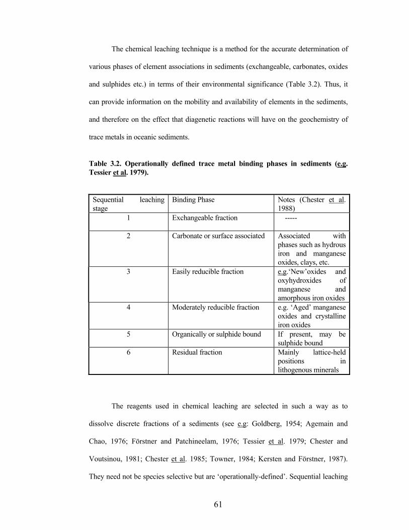
The chemical leaching technique is a method for the accurate determination of
various phases of element associations in sediments (exchangeable, carbonates, oxides
and sulphides etc.) in terms of their environmental significance (Table 3.2). Thus, it
can provide information on the mobility and availability of elements in the sediments,
and therefore on the effect that diagenetic reactions will have on the geochemistry of
trace metals in oceanic sediments.
Table 3.2. Operationally defined trace metal binding phases in sediments (e.g.Tessier et al. 1979).
Sequential leaching stage
Binding Phase Notes (Chester et al.1988)
1 Exchangeable fraction -----
2 Carbonate or surface associated Associated with phases such as hydrous iron and manganese oxides, clays, etc.
3 Easily reducible fraction e.g.‘New’oxides and oxyhydroxides of manganese and amorphous iron oxides
4 Moderately reducible fraction e.g. ‘Aged’ manganese oxides and crystalline iron oxides
5 Organically or sulphide bound If present, may be sulphide bound
6 Residual fraction Mainly lattice-held positions in lithogenous minerals
The reagents used in chemical leaching are selected in such a way as to
dissolve discrete fractions of a sediments (see e.g: Goldberg, 1954; Agemain and
Chao, 1976; Förstner and Patchineelam, 1976; Tessier et al. 1979; Chester and
Voutsinou, 1981; Chester et al. 1985; Towner, 1984; Kersten and Förstner, 1987).
They need not be species selective but are ‘operationally-defined’. Sequential leaching

62
studies can distinguish between the distribution of metals in the detrital (or refractory)
and non-detrital (or non-refractory) fractions of sediments (see e.g: Chester and
Messiha-Hanna, 1970, Chester and Voutsinou, 1981). Trace metals associated with the
detrital fractions are held in the internal matrix structure of aluminosilicate and other
detrital minerals, whilst the non-detrital fractions of metals are fixed in a number of
non-matrix associations, some of which are more stronger than others. A two stage
leaching technique that distinguishes between detrital and non-detrital metals can be
applied as a rapid and simple method to obtain information on the storage of elements
and the detection of the degree of metal pollution in sediments, but it will mask any
subtle geochemical associations in the non-detrital fraction itself. Multi-stage
sequential leaching techniques are therefore often employed, and have been extensively
reviewed by Towner (1984) and Thomas (1987). The scheme applied in this study
(Table 3.3) is the ‘best working compromise’, linking operationally-defined host
separations with geochemically meaningful fractions. The scheme was initially
proposed by Tessier et al. (1979) and modified later by Towner (1984) and Thomas
(1987) (see Table 3.2). The modifications of the schemes were as follows:
1) The magnesium chloride reagent (stage 1) was replaced by ammonium
acetate, because the former attacks carbonates (Tessier et al. 1979; Towner, 1984). The
use of ammonium acetate also alleviates the more serious matrix problems encountered
with magnesium chloride in GF-AAS; e.g. interference in lead determinations as a
result of the formation of lead chlorides in the graphite furnace (Sturgen and
Chakrabarti, 1978).
2) An additional step (stage 3) was incorporated into the scheme to differentiate
between the easily reducible fraction (mainly manganese oxy-hydroxides with small
amounts of amorphous iron oxides) and the moderately reducible fractions (mainly
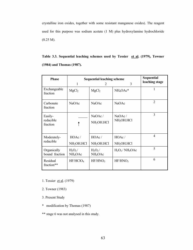
63
crystalline iron oxides, together with some resistant manganese oxides). The reagent
used for this purpose was sodium acetate (1 M) plus hydroxylamine hydrochloride
(0.25 M).
Table 3.3. Sequential leaching schemes used by Tessier et al. (1979), Towner
(1984) and Thomas (1987).
Phase Sequential leaching scheme 1 2 3
Sequential leaching stage
Exchangeablefraction
MgCl2 MgCl2 NH4OAc* 1
Carbonate fraction
NaOAc NaOAc NaOAc 2
Easily-reduciblefraction
NaOAc /
NH2OH.HCl
NaOAc / NH2OH.HCl
3
Moderately-reducible
HOAc /
NH2OH.HCl
HOAc /
NH2OH.HCl
HOAc /
NH2OH.HCl
4
Organicallybound fraction
H2O2 /NH4OAc
H2O2 /NH4OAc
H2O2 / NH4OAc 5
Residualfraction**
HF/HClO4 HF/HNO3 HF/HNO36
1. Tessier et al. (1979)
2. Towner (1983)
3. Present Study
* modification by Thomas (1987)
** stage 6 was not analysed in this study.
64
3.1.2. Cleaning Procedure
All glassware and polypropylene boiling tubes were cleaned by soaking in an
acid bath (10% HNO3 , 24 h), rinsed with Milli-Q water (18.2 M cm-1) and dried in an
oven (~600C). Volumetric flasks and graduated measuring cylinders were treated in the
same way but dried at room temperature.
3.1.3. Chemicals
The following chemicals were used for sequential leaching:
1) Milli-Q water (18 M cm-1 resistivity) was used for the reagents and standard
preparations.
2) Nitric acid (16 M ; AnalaR grade), BDH. This reagent was purified by redistillation
of ‘AnalaR’ grade acid in a distillation apparatus fitted with a quartz stillhead and
condenser. The redistilled concentrated acid was then diluted to 0.1 M with Milli-Q
water and was used for making up extractants and standards.
3) Ammonium acetate (1 M ; AnalaR grade, BDH).
4) Sodium acetate (1 M ; AnalaR grade, BDH).
5) Hydroxylamine hydrochloride (25 % ; AnalaR grade, BDH).
6) Hydrogen Peroxide (30% ; AnalaR grade, BDH).
7) Acetic acid (Redistilled; AnalaR grade, BDH). This reagent was purified by
redistillation of ‘AnalaR’ BDH grade acid (as above).

65
3.1.4. Apparatus
1) Volumetric flasks (25 mL) were used for making up the standard and extractants to
known volumes.
2) Polypropylene boiling tubes (50 mL) were used for the extraction procedure.
3) Pre-cleaned polyethylene containers were used for storage of reagents.
4) Linear polystyrene (‘Sterilin’) bottles (30 mL) were used for storage of samples and
standards prior to analysis.
5) A Janke & Kunkel (IKA - Labortechnik KS 501D) mechanical orbital shaker was
used to agitate samples to ensure uniform reaction of sample and reagent .
6) A MSE ‘Centaur 1’ centrifuge was used (3000 r.p.m) for the separation of the residue
from the solution where necessary.
7) A sand bath was used to heat samples for Stages 4 and 5 at the required temperature.

66
3.1.5. Reagent Preparation
(Stage 1) Surface adsorbed, or exchangeable, ions
Preparation of ammonium acetate solution (1 M)
Ammonium acetate (77 g) was dissolved in water (Milli-Q, 1000 mL) and the
reagents were passed through a 10 cm ion exchange column containing ‘Chelex 100’
resin in the ammonium form, to remove any trace metals present. The pH of the solution
was then adjusted to 7.0 with redistilled acetic acid.
(Stage 2) Carbonate-associated and chemi-sorbed ions
Preparation of sodium acetate solution (1 M)
Sodium acetate (136.08g) was dissolved in water (Milli-Q, 1000 mL) and
cleaned as for stage 1. The pH of the reagent was then adjusted to 5.0 with redistilled
acetic acid.
(Stage 3) Easily reducible (manganese) oxides
Preparation of hydroxylamine hydrochloride (0.25 M)/Sodium acetate solution
(1 M)
Hydroxylamine hydrochloride (17.4 g) was added to sodium acetate (1 M)
dissolved in water (Milli-Q, 1000 mL). The pH was adjusted to 5.0 with redistilled
acetic acid.
67
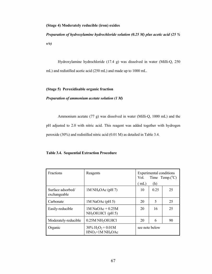
(Stage 4) Moderately reducible (iron) oxides
Preparation of hydroxylamine hydrochloride solution (0.25 M) plus acetic acid (25 %
v/v)
Hydroxylamine hydrochloride (17.4 g) was dissolved in water (Milli-Q, 250
mL) and redistilled acetic acid (250 mL) and made up to 1000 mL.
(Stage 5) Peroxidisable organic fraction
Preparation of ammonium acetate solution (1 M)
Ammonium acetate (77 g) was dissolved in water (Milli-Q, 1000 mL) and the
pH adjusted to 2.0 with nitric acid. This reagent was added together with hydrogen
peroxide (30%) and redistilled nitric acid (0.01 M) as detailed in Table 3.4.
Table 3.4. Sequential Extraction Procedure
Fractions Reagents Experimental conditions Vol. Time Temp.(oC)( mL) (h)
Surface adsorbed/ exchangeable
1M NH4OAc (pH 7) 10 0.25 25
Carbonate 1M NaOAc (pH 5) 20 5 25
Easily-reducible 1M NaOAc + 0.25M NH2OH.HCl (pH 5)
20 16 25
Moderately-reducible 0.25M NH2OH.HCl 20 6 90
Organic 30% H2O2 + 0.01M HNO3+1M NH4OAc
see note below

68
3.1.6. Sequential Leaching Extraction Procedure
A dried sediment sample was homogenised using a pestle and mortar, then the
sample (~50-200 mg) was accurately weighed into a polypropylene boiling tube. The
first reagent (stage 1, 10 mL) was added to the sample and the tube covered with a piece
of clingfilm in order to avoid contmination from the cap. Care was taken to allow
minimal contact between the reagent and the clingfilm and the tube was shaken on a
mechanical shaker (15min; 25oC). The polypropylene tube was then centrifuged (15
min; 3000 r.p.m). The supernatant liquid was decanted into a volumetric flask and made
up to volume with redistilled HNO3 (0.1 M; stage1, 10 mL and stage 2-5, 25 mL). The
respective leaching solutions were transferred after each stage into Sterilins tubes (30
mL) for storage prior to analysis.
The remaining solid residue after each stage was treated, respectively, with the
next stage reagent. A similar method of shaking and centrifuging was followed as
mentioned below (see Table 3.4).
Stage 2 reagent (20 mL) was added to the stage 1 residue in the boiling tube, and
the tube was shaken on a mechanical shaker (5 h ; 25o C ) and then centrifuged (15
min.).
Stage 3 reagent (20 mL) was added to the stage 2 residue in the boiling tube, and
the tube was shaken on a mechanical shaker (16 h; 25o C) and then centrifuged (15
min.).
Stage 4 reagent (20 mL) was added to the stage 3 residue in the boiling tube, and
heated in a sand bath (90o C ; 6 h).
For Stage 5, H2O2 (5 mL) and HNO3 ( 0.01 M; 3 mL) were added to the residue
in the boiling tube and heated (85oC ; 2 h), after which further portions of H2O2 (3 mL)
69
and HNO3 (0.01 M; 2 mL) were added and samples heated (85oC; 3 h). The solutions
were allowed to cool prior to addition of NH4OAc (1 M; 10 mL). The tubes were shaken
continually (16 h) and centrifuged.
Extractions were performed along with in-house standard reference materials
and analyses was carried out within two days of the extraction of leached elements.
3.1.7. Preparation of Standard Solutions
Mixed (multi-element) standards were made up from BDH ‘Spectrosol’ stock
solutions (1000 ppm) in a redistilled nitric acid (0.1 M) matrix and stored in ‘Sterilin’
containers until required. An initial mixed standard (100 ppm) was made up and then
aliquots were diluted with respective sequential leaching solutions to give a range of
standards (10, 20, 50 ppb, 0.1, 0.2, 0.5, 1.0 and 2.0 ppm) in Sterilin bottles. Because of
the large number of sample analyses involved, it was not possible to adopt a standard
additions method to eliminate matrix effects. Instead, sample and standard matrices
were closely matched (e.g. Lachica and Barahona, 1993). For this purpose, a range of
standard solutions was prepared using the following matrices which correspond to the
individual sequential extraction stages.
(Stage 1) Ammonium acetate solution (1 M).
(Stage 2) Sodium acetate solution (1 M).
(Stage 3) Hydroxylamine hydrochloride (0.25 M)/Sodium acetate solution (1 M).
(Stage 4) Hydroxylamine hydrochloride solution (0.25 M) plus acetic acid (25 % v/v).
(Stage 5) Ammonium acetate solution (1 M)+Hydrogen peroxide (30%) and redistilled
nitric acid (0.01 M).

70
The standards were all handled in a dust-free room with critical stages of
preparation being performed in a clean air cabinet. Autopipettes were used to transfer
quantities of the standards, with appropriate changes of pipette tips to avoid
contamination.
3.1.8. Instrumentation
3.1.8.1. Flame AAS
All determinations of Mn and Fe were made on a Perkin-Elmer model 2380
flame atomic absorption spectrophotometer. The analytical conditions are shown in
Table 3.5. All the flame measurements were made on a double beam dual channel (i.e.
both the hollow cathode lamp (or EDL) and the BG deuterium arc lamp are present)
using single element hollow cathode lamps. This has the capability of simultaneous
background correction using a deuterium lamp. For the determination of Mn, Fe and Cu
(if above detection limits) concentration, an air-acetylene flame was used.
Table 3.5. Instrumental Conditions for the Perkin-Elmer 2380 AAS.*
Flame AAS
Element Wavelength (nm)
Slit width (nm)
Flame Sensitivity (ppm)
Linearrange(ppm)
Manganese 279.5 0.2 Air- acetylene
0.052 (FS) 0.030 (IB)
2.0 (FS) 2.0 (IB)
Iron 248.3 0.2 Air-acetylene
0.100 (FS) 0.039 (IB)
5.0 (FS) 2.0 (IB)
Copper 324.8 0.7 Air-acetylene
0.077 (FS) 0.032 (IB)
5.0 (FS) 2.0 (IB)

71
Note FS - Flow Spoiler ; IB - Impact Bead
* as recommended in the manufacturer manual (Perkin-Elmer).
Both the standard and sample solutions were aspirated directly into the flame,
but dilutions were made whenever the sample concentrations were beyond the upper
limit of the linear range.
Calibration curves were constructed from known standards (in an appropriate
matrix) to obtain the linear working range for individual elements in each matrix. The
calibration curves were re-determined periodically (ca. every 6 samples) to check for
drift in the baseline during a series of determinations. Blanks were run together with
each batch of samples to take into account reagent, or other, sources of contamination.
Where blank readings were significant, these were subtracted from the concentrations
obtained for the sample.
3.1.8.2. Graphite AAS
Copper was generally present in low concentrations which required the use of
graphite furnace AAS. A Perkin-Elmer AAS (Model 1100 B) equipped with deuterium
background correction, an AS-70 auto sampler, HGA 700 furnace programmer and
EPSON.FX-850 Printer Sequencer was used. Single element hollow cathode lamps
were employed and argon was used as the carrier gas. The appropriate wavelengths,
lamp currents and other conditions for the determination of Cu were selected from the
Perkin-Elmer reference manual as a guide in developing the program conditions.
However, the optimum temperature and time required for a particular stage in a
72
particular matrix, was used to obtain the maximum sensitivity and/or greatest working
(linear) range for Cu (see Appendix A).
Calibration curves were constructed from known standards (in the appropriate
matrix) to obtain the working range for Cu in each matrix. In graphite furnace AAS,
matrix matching of samples and standards is very important, since the technique suffers
from matrix affects, even though in theory, the matrix is removed before the sample is
atomised. Apart from this, ‘memory effects’ found between individual determinations,
may arise during the use of graphite furnace due to metal impactions onto graphite tube
walls. The use of pyro-coated graphite tubes and appropriate programmes reduces this
problem. The pyro-coated tubes have also been found to be more resistant to corrosive
matrices and severe temperature programs selected (e.g.) to volatise Na+ in stages 2 and
3), and to have longer life spans.
Reagent blanks were run concurrently with samples to check for any possible
reagent, or other operationally associated, contamination. Necessary corrections were
made in the determination of sample concentration, where significant blank values were
observed.
3.1.9. Determination of Trace Metals
The following equation was used to calculate the concentration of each element
in the sediment sample.

73
CE = (AxB)/SW g/g
CE = Concentration of element ( g/g)
A = Concentration of element in solution ( g/mL)
B = Volume of extracted solution (mL)
SW = Sediment weight (g)
3.1.10. Reproducibility
Analytical reproducibility was determined by duplicate analyses of extracts of
in-house standard reference materials which were analysed routinely with each batch of
samples. A Mersey sediment used for this purpose was originally prepared by mixing
and homogenising several sediment samples collected from the River Mersey. The
analytical development and reproducibility experiments have been carried out
previously in these laboratories by a number of workers.
The analytical precision of the sequential leaching scheme (Table 3.3) was
determined by sequential analysis of a Mersey sediment (in duplicate) and the results are
reported below (see Table 3.6).
74
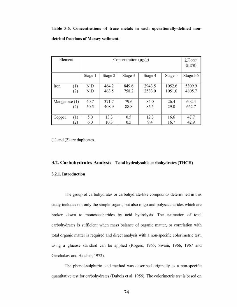
Table 3.6. Concentrations of trace metals in each operationally-defined non-
detrital fractions of Mersey sediment.
Element Concentration (µg/g) Conc. (µg/g)
Stage 1 Stage 2 Stage 3 Stage 4 Stage 5 Stage1-5
Iron (1) (2)
N.DN.D
464.2 463.5
849.6 758.2
2943.5 2533.0
1052.6 1051.0
5309.9 4805.7
Manganese (1) (2)
40.7 50.5
371.7 408.9
79.6 88.8
84.0 85.5
26.4 29.0
602.4 662.7
Copper (1) (2)
5.06.0
13.3 10.3
0.5 0.5
12.3 9.4
16.6 16.7
47.7 42.9
(1) and (2) are duplicates.
3.2. Carbohydrates Analysis - Total hydrolysable carbohydrates (THCH)
3.2.1. Introduction
The group of carbohydrates or carbohydrate-like compounds determined in this
study includes not only the simple sugars, but also oligo-and polysaccharides which are
broken down to monosaccharides by acid hydrolysis. The estimation of total
carbohydrates is sufficient when mass balance of organic matter, or correlation with
total organic matter is required and direct analysis with a non-specific colorimetric test,
using a glucose standard can be applied (Rogers, 1965; Swain, 1966, 1967 and
Gerchakov and Hatcher, 1972).
The phenol-sulphuric acid method was described originally as a non-specific
quantitative test for carbohydrates (Dubois et al. 1956). The colorimetric test is based on

75
the formation of an orange complex on reaction of phenol, sulphuric acid and a
carbohydrate. It is often preferred for total carbohydrate analysis, because its molar
absorptivities for most sugars fall within a narrow range; unlike those observed for
various sugars by other methods. The phenol-sulphuric acid method has been used for
the determination of total carbohydrates in sediments (Artem’yev, 1969, 1970) and in
particulate matter (Handa, 1967) after hydrolysis (Dubois et al. 1956; modified by
Gerchakov and Hatcher, 1972), with spectrophotometric monitoring at a wavelength of
485 nm (see Fig. 3.1). Handa (1966) suggested the phenol method for the determination
of carbohydrates in seawater was more accurate, rapid and reliable than either N-
ethylcarbazole, or anthrone methods. Artem’yev (1969) examined the phenol method
for the determination of the total content of carbohydrates in sediments and came to
similar conclusions. Many other authors have adopted this method (e.g.
Artem’yev,1970; Dubois et al. 1956; Faganeli et al. 1987; Gerchakov and Hatcher,
1972; Hitchcock, 1977; Tanoue, 1985) in preference to analysis of individual
monosaccharides (e.g. by Brockmann, 1982; Cowie and Hedges, 1984a, b; Hamilton
and Hedges, 1988; Handa and Mizuno, 1973; Ittekkot et al. 1984a; Klok et al. 1983;
Liebezeit, 1986; Mopper, 1977; Rogers, 1965; Steinberg et al. 1987; Uzaki and
Ishiwatari, 1983; Yamaoka, 1983a).


78
3.2.3. Chemicals
The chemicals used for the carbohydrates determinations were as follows:
Milli-Q water for the reagents and standards preparations.
Potassium hydroxide (Fisons Analytical Reagents).
Concentrated Sulphuric acid (‘AnalaR’ grade, BDH).
Phenol (‘AnalaR’ grade, BDH).
Glucose (‘AnalaR’ grade, BDH).
3.2.4. Apparatus
Pyrex culture tubes with screw topped and teflon lined were used for hydrolysis
of carbohydrates.
Conical flasks (50 mL).
Volumetric flasks (25 mL).
‘Centaur 1’ centrifuge (MSE).
3.2.5. Reagent Preparation
Preparation of standard solution
A standard glucose stock solution (~550 M) for carbohydrate analysis was
prepared by dissolution of glucose (25 mg) in water (Milli-Q, 250 mL) and this was
used to make a series of standard solutions (~27.5-550 M) in water (Milli-Q, 25 mL).
Preparation of Phenol solution
79
Phenol solution (0.53M) was prepared by dissolution of phenol (12.5 g) in water
(Milli-Q, 250 mL).
Preparation of Potassium hydroxide solution
Potassium hydroxide solution (0.1M) was prepared by dissolution of potassium
hydroxide (1.4 g) in water (Milli-Q, 250 mL).
3.2.6. Extraction of Carbohydrates
The freeze dried and homogenised sediment (~100-200 mg) was weighed in
duplicate into clean pre-weighed Pyrex culture tubes (16 x 150 mm), which were sealed
with teflon-lined screw caps. A procedural blank of water (Milli-Q, 1 mL) was also
included in every batch, H2SO4 was then added to the tube (1 mL ; 12 M) and the
solution left to stand (2 h) at room temperature. The sample was then diluted (1M) with
water (Milli-Q) and hydrolysed (4.5 h ; 100-1200 C) in an oven, after which it was
allowed to cool. The hydrolysate was centrifuged (3000 r.p.m) and transferred into a
conical flask, prior to freezing and freeze-drying (Modulyo Freeze Drier and E2M8
High Vacuum Pump; Edwards). The hydrolysate was redissolved in KOH solution (0.1
mol/L) and made up to 25 mL. The sediment residue left after the first hydrolysis was
rehydrolysed as above. The samples were then determined separately for
monosaccharide contents.
80
3.2.7. Determination of Carbohydrates
In the present study, the determination of carbohydrates was carried out after
hydrolysis, using the phenol-sulphuric acid method (Patience et al. 1990). The details of
the analytical method are described below and also shown in Fig. 3.3.
Three aliquots of each standard (2 mL); (27.5 - 550 M) were transferred to a
series of conical flasks, labelled Ai, Bi and Ci. Phenol solution (2 mL) and sulphuric
acid (10 mL) was added to the ‘A’ series. Water (Milli-Q, 2 mL) and sulphuric acid (10
mL) was added to the ‘B’ series. Phenol (2 mL) and water (Milli-Q, 10 mL) was added
to the ‘C’ series. All additions were made with rapid mixing. Sediment samples
(hydrolysate) were treated identically to the standards.
The solutions were transferred to 1 cm cuvettes, and the absorbances read at 485
nm. Absorbances of the ‘A’ series were measured vs. those of the ‘B’ series. Phenol
absorbance was corrected by measuring the absorbance of the ‘C’ series vs. a blank
containing water (Milli-Q, 12 mL) and phenol (2 mL).
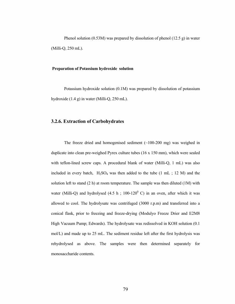
A standard curve of corrected absorbance at 485 nm (‘A’ vs. ‘B’) - ‘C’ vs.
glucose standard concentration was constructed (Fig.3.4) and the glucose-equivalent
concentrations (mM) in sediment samples were then determined and converted to mol
g-1 dry sediment weight or mol (g TOC)-1.

81
VOLUME REDUCTION
Freeze - drying
Homogenize (~0.2 g)
Hydrolysate (frozen)
DRY SEDIMENT
ACID HYDROLYSIS
FROZEN SEDIMENT-CORE SECTIONED AT 10 & 20 mmINTERVALS
Derivatization (0.1 mol/L KOH)
Phenol-Sulphuric acid method Ninhydrin method
Free monosaccharides Free amino acids
UV/VIS SPECTROPHOTOMETRY
@485 nm @570 nm
Total hydrolysable carbohydrate (THCH)
Total hydrolysable amino acids(THAA)
(12M H2SO4 - THCH)/ (6N HCl - THAA)
(Freeze - drying)
Fig. 3.3. Flow chart of carbohydrate and protein analytical methods
82
R2 = 1
0
0.1
0.2
0.3
0.4
0.5
0.6
0.7
0 100 200 300 400 500
Concentration of Glucose standard (µM)
Abs
orba
nce
@ 4
85 n
m
Fig. 3.4. Calibration curve of aqueous Glucose standard.
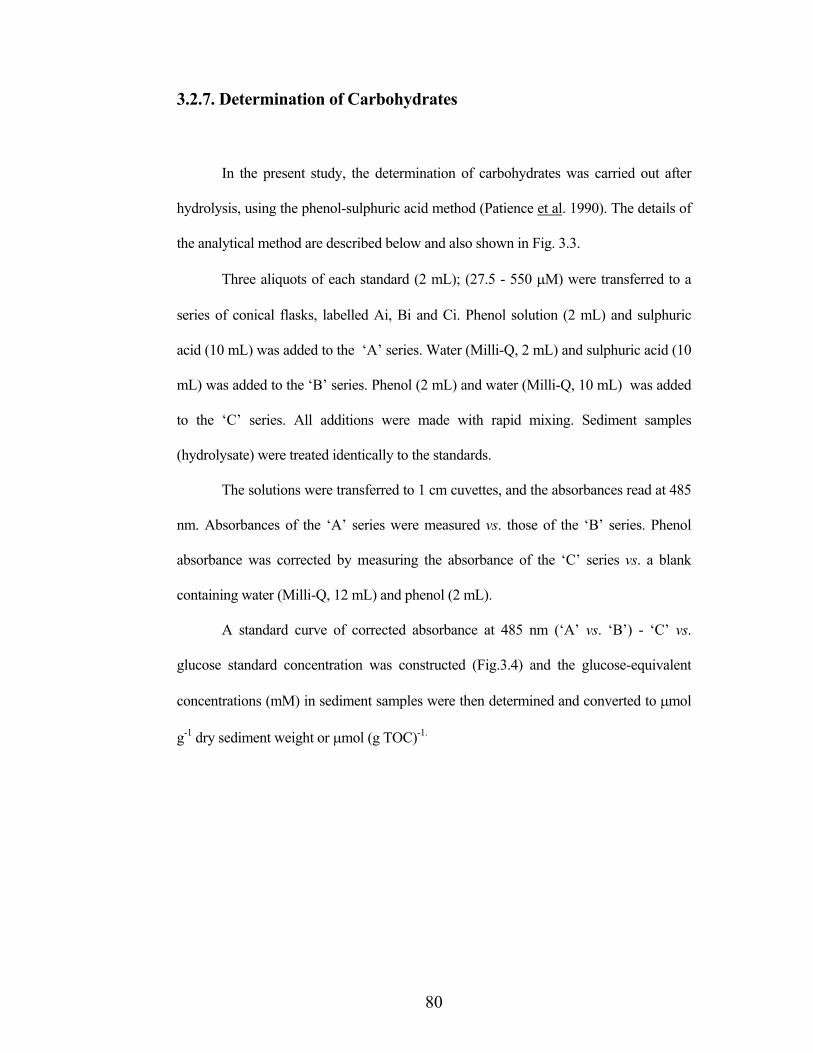
3.2.8. Reproducibility
In the present study, experiments were carried out to determine the
reproducibility of the analytical procedure for carbohydrates using starch as a standard.
The efficiency of the hydrolysis procedure was also determined and the results were
compared with those for a characterised standard sediment sample (Cargreen mud,
Tamar Estuary, UK; supplied by Prof. S. J. Rowland).
83
3.2.8.1. Preparation of starch solution
Standard starch solution (0.5 mg/mL) was prepared by dissolving starch (50 mg)
in hot water (Milli-Q) and dilution to 100 mL. A series of working standards were
prepared by diluting aliquots of the stock to obtain the range of concentrations (50-500
mg/mL). A known volume (5 mL; in duplicate) of each solution was pipetted out into
clean Pyrex tubes. These solutions were then frozen and freeze-dried.
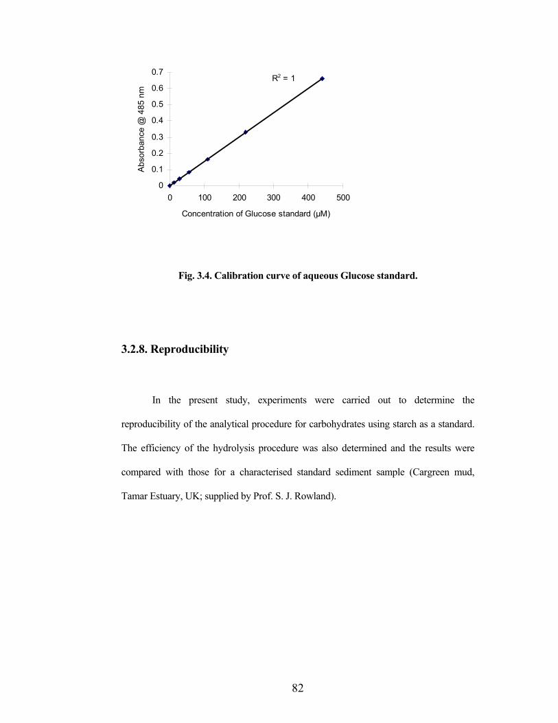
3.2.8.2. Analysis of starch solution
Hydrolyses were carried out on the dried samples and monosaccharide contents
determined. The calibration curve for starch solution (Fig.3.5) showed a similar linear
relationship to that of the calibration curve of the glucose standard (Fig.3.4).
R2 = 0.9838
R2 = 0.9961
-10
0
10
20
30
40
50
60
70
80
90
0 10 20 30 40 50 60 70 80 90 100
Concentration of Starch (µg/mL)
Con
c.of
equ
ival
ent G
luco
se re
spon
se (µ
g/m
L)
Replicate1
Replicate 2
Fig. 3.5. Calibration curve of aqueous starch solution.
3.2.8.3. Analysis of sediment samples

84
2 gram Cargreen sediment (with conc. 62.9 mol/g) were spiked with 2 mg of
starch solution. The replicate analyses (n = 6) yielded the carbohydrates concentrations
which were reproducibile to ±10%.
3.2.9. Efficiency of hydrolysis
The efficiency of the hydrolysis procedure for THCH was determined by
sequential hydrolysis and analysis of a Arabian Sea abyssal sediment sample. The
sediment (~0.2 g) was sequentially hydrolysed (x 4); >90% of THCH was released in
the first hydrolysis. No carbohydrates were detected in the third and fourth hydrolysis.
Hence in this study, two hydrolyses (in duplicate) were carried out and the sample
concentrations combined.
3.3. Protein Analysis
(Total hydrolysable amino acids -THAA)
3.3.1. Introduction
There are a number of methods for the quantification of total proteins (for a
review, see Davies, 1988), with the most frequently cited method being that of Lowry et
al. (1951). Unfortunately, the Lowry assay suffers from interference by a number of
compounds, including free amino acids (Peterson, 1979). Mayer et al. (1986) developed
a method for measuring the enzymetically available protein content of sediments. The
method was developed to measure total bioavailable protein, available to deposit

85
feeders. The current techniques for total protein estimation are sensitive to a variety of
interfering compounds, which often compromise accurate measurements.
The determination of proteins in recent sediments can be carried out after
hydrolysis by characterization of individual amino acids (Degens et al. 1964; Henrichs
and Farrington, 1987; Henrichs et al. 1984; Ittekkot et al. 1984a; Klok et al. 1983;
Maita et al. 1982; Morris, 1975; Müeller et al. 1986; Rosenfeld, 1979; Steinberg et al.
1987; Whelan, 1977) or by quantification using a bulk amino acid assay, such as the
ninhydrin method (Rosen, 1957) used here and previously by various authors
(Greenfield et al. 1970; Stevenson and Cheng, 1970). The advantage of the latter
method is that it is much easier, quicker, and cheaper; the disadvantage is that it
quantifies amino groups, not amino acids. The absolute results presented here may thus
include a small proportion of compounds that are not amino acids, but which react in the
assay, if any such compounds are present.
The ninhydrin test is a colorimetric method involving the formation of a purple
colour from the reaction of reduced ninhydrin and amine groups (Rosen, 1957). Amino
acids were quantified using a calibration curve set up using known concentrations of
glycine. The response variations for different amino acids are negligible, and corrections
are not required.
86
3.3.2. Cleaning Procedure
The apparatus were cleaned in a similar way to that employed for the
carbohydrate analysis.
3.3.3. Chemicals
The chemicals used for the determination of proteins are as follows:
Milli-Q water for the reagents and standards preparations.
Stock Sodium Cyanide (0.01 M), ( Aldrich, A.C.S Reagent) .
Potassium hydroxide ( Fisons Analytical Reagent ).
Sodium Acetate (AnalaR grade, BDH).
Acetic acid (glacial, AnalaR grade, BDH).
Ninhydrin ( Aldrich, A.C.S Reagent).
2-Methoxy ethanol ( Aldrich, Spectrophotometric grade).
2-Propanol (BDH-Hipersolv).
Glycine (AnalaR grade, BDH).
3.3.4. Apparatus
Pyrex culture tubes with teflon-lined screw caps and were used for hydrolyses of
proteins.
Conical flasks (50 mL).
Volumetric flasks (25 mL).
Centaur centrifuge.
87
3.3.5. Reagent Preparation
Preparation of glycine standard solutions
A standard glycine stock solution (10 mM) was prepared by dissolution of
glycine (75 mg) in water (Milli-Q, 100 mL) and used to make up a range of
concentrations (0.04-0.4 mM).
Preparation of stock Sodium cyanide solution
Sodium cyanide solution (0.01 mol/L) was prepared by dissolution of sodium
cyanide (122.5 mg) in water (Milli-Q, 250 mL).
Preparation of Acetate Buffer
Sodium acetate solution (3.96 M) was prepared by dissolving sodium acetate
(NaOAc.3H2O; 54 g) in water (Milli-Q) with addition of glacial acetic acid (10 mL).
The final solution was made up to 100 mL.
88
Preparation of Acetate/Cyanide Buffer
Sodium cyanide in acetate buffer solution (0.2 mM) was prepared by diluting
sodium cyanide (1 mL ; 0.01mol/L) in acetate buffer (50 mL).
Preparation of Ninhydrin solution
Ninhydrin solution (3% wt./vol.) was prepared by dissolving ninhydrin (1.5 g) in
methylcellosolve (50 mL).
Preparation of Diluent (2-Propanol/Water, 1:1)
2-Propanol (125 mL) was mixed with water (125 mL) and made up to 250 mL.
Preparation of Potassium hydroxide solution
Potassium hydroxide solution was prepared by dissolving potassium hydroxide
(1.4 g) in water (Milli-Q, 250 mL).
3.3.6. Extraction of Proteins
The freeze dried and homogenised sediment (100-200 mg) was weighed, (in
duplicate), into clean pre-weighed Pyrex culture tubes with teflon-lined screw caps
(16x150 mm). A procedural blank (1 mL, Milli-Q water) was also included with each
batch of samples. Then HCl was added (1 mL; 6 M) and hydrolysed in an oven (24 h,

89
100o C). The samples were removed from the oven and allowed to cool, added water (10
mL, Milli-Q) into the sample, after which the hydrolysates were centrifuged (3000
r.p.m) and transferred into conical flasks prior to freezing and freeze-drying (Modulyo
Freeze Drier and E2M8 High Vacuum Pump; Edwards). The hydrolysates were
redissolved in KOH solution (0.1 mol/L) and made up to 25 mL. The sediment residues
remaining after the first hydrolysis were rehydrolysed as above. The samples were then
analysed separately for protein content.
3.3.7. Determination of Proteins
Two aliquots of each standard (1 mL each; 0.04, 0.1, 0.2, 0.3, 0.4 mM), reagent
blank and sediment samples (hydrolysate) were transferred into series of Pyrex culture
tubes labelled as ‘Ai’ and ‘Bi’. To the ‘A’ series were added acetate-cyanide (0.5 mL)
and ninhydrin solution (0.5 mL). The tubes were immediately capped (loosely) and
placed in a sand bath (100oC; 15 min.). After removal from the sand bath, the diluent (2-
propanol/water; 10 mL) was added to each of the tubes, which were then shaken and
allowed to cool to room temperature. The tubes were then centrifuged for 20 minutes to
remove suspended particles that might affect absorbance readings. Aliquots of each
solution were then transferred to a 1 cm cuvette, and the absorbance measured at 570
nm vs. the reagent blank. A calibration curve of absorbance vs. concentration was
constructed using the standards. To account for any indigenous colour present in the
final reacted unknown solutions, a second set of aliquots (1 mL) of the unknowns were
collected in the ‘B’ series. To these solutions was added water (0.5 mL) and
methylcellosolve (0.5 mL); the resulting solutions were heated as before. Recorded
absorbances were measured vs. a water blank (1.5 mL H2O, 0.5 mL methylcellosolve

90
and 10 mL diluent) and the net absorbance subtracted from the value for the reacted
solution. The measured absorbance of unknown samples was corrected by subtraction of
the blank absorbance values.
A standard curve of corrected absorbance at 570 nm vs. glycine standard
concentration was constructed (Fig. 3.6) and the glycine-equivalent concentration (mM)
in the samples was then calculated. The concentrations of sediment samples were
converted to mol g-1 dry sediment weight.
R2 = 0.9977
0
0.1
0.2
0.3
0.4
0.5
0.6
0.7
0 0.05 0.1 0.15 0.2 0.25 0.3 0.35 0.4
Concentration of Glycine standard (mM)
Abs
orba
nce
@ 5
70 n
m
Fig. 3.6. Calibration curve of aqueous glycine standard.
91
3.3.8. Reproducibility
In order to determine the reproducibility of the analytical procedure a
myoglobin-standard was subjected to the hydrolysis and analytical procedures. The
efficiency of the hydrolysis was also determined and the results were compared with
those for a standard sediment sample (Cargreen mud, Tamar Estuary, UK; supplied by
Prof.S.J. Rowland).
3.3.8.1. Preparation of myoglobin solution
Standard myoglobin solution (0.5, 0.1 mg mL-1) was prepared by dissolution of
myoglobin (50, 10 mg) in water (Milli-Q,100 mL). A series of working standards were
prepared from the stock solutions to obtain the range of concentration (50-500 mg mL-1;
10-100 mg mL-1). A known volume (5 mL; in duplicate) of each solution was pipetted
into a clean Pyrex tube. These samples were then frozen and freeze-dried.
3.3.8.2. Analysis of myoglobin solution
Hydrolyses were carried out on the dried samples, and resultant solutions were
analysed for protein content as mentioned in section 3.3.7. The calibration curve of
myoglobin solution (Fig.3.7) showed a linear relationship similar to that of the glycine
standard (Fig.3.6).
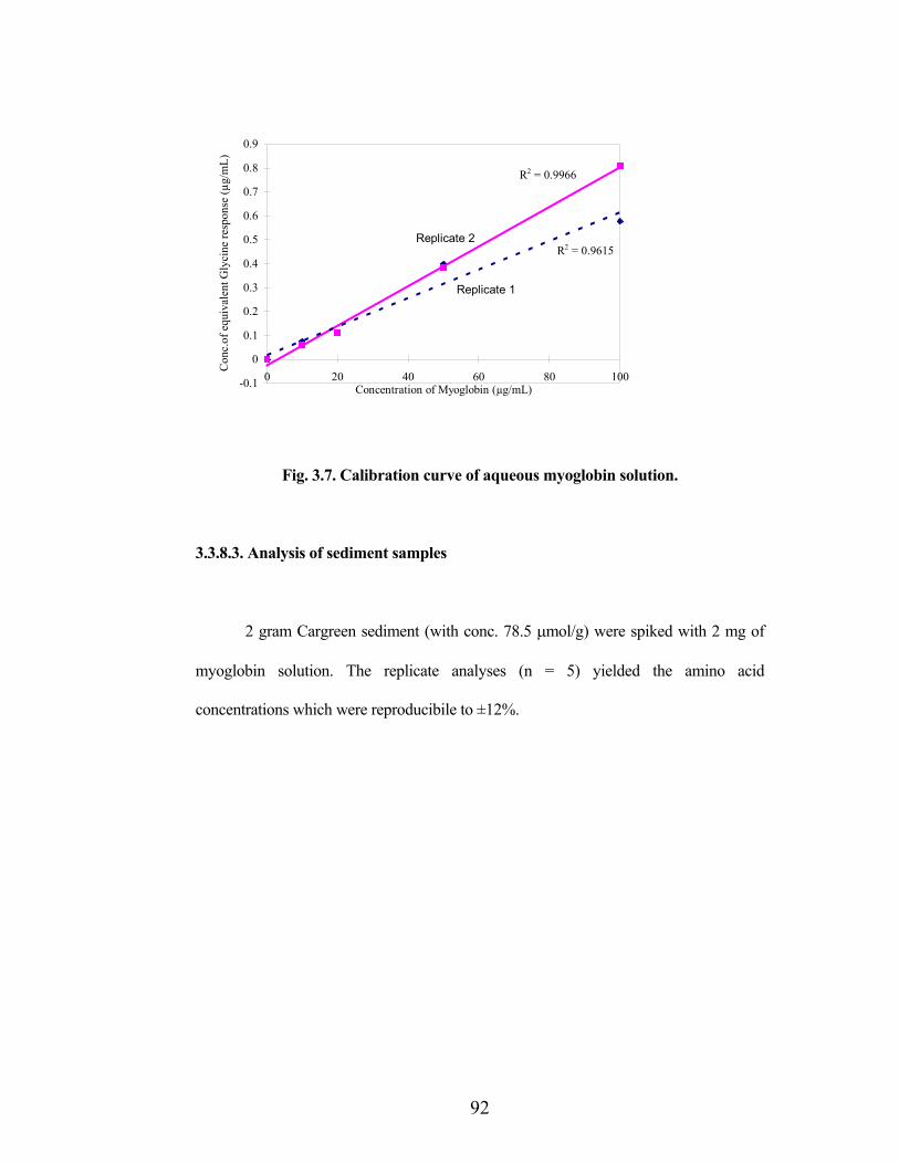
92
R2 = 0.9966
R2 = 0.9615
-0.1
0
0.1
0.2
0.3
0.4
0.5
0.6
0.7
0.8
0.9
0 20 40 60 80 100Concentration of Myoglobin (µg/mL)
Con
c.of
equ
ival
ent G
lyci
ne re
spon
se (µ
g/m
L)
Replicate 1
Replicate 2
Fig. 3.7. Calibration curve of aqueous myoglobin solution.
3.3.8.3. Analysis of sediment samples
2 gram Cargreen sediment (with conc. 78.5 mol/g) were spiked with 2 mg of
myoglobin solution. The replicate analyses (n = 5) yielded the amino acid
concentrations which were reproducibile to ±12%.

93
3.3.9. Efficiency of hydrolysis
The efficiency of the hydrolysis procedure for THAA was determined by
sequential hydrolysis and analysis of a Arabian Sea abyssal sediment sample. The
sediment (~0.2 g) was sequentially hydrolysed (x 4); >90% of THAA was released in
the first hydrolysis. No amino acids were detected in the third and fourth hydrolysis.
Hence in this study, two hydrolyses (in duplicate) were carried out and the sample
concentrations combined.
3.4. Elemental Analyses
3.4.1. Instrumentation
The elemental compositions of C, H and N of samples in the present study were
determined using a Carlo Erba Strumentazine Elemental Analyser model 1106. This
instrument performs CHN analyses by combustion of samples in the presence of
chromic oxide and copper oxide (10280 C) yielding CO2, H2O and a mixture of nitrogen
oxides. A secondary reaction tube (containing Cu) removes excess oxygen and reduces
nitrogen oxide to nitrogen. The resultant gases are then passed through GC separatory
column (2 M Porapak Q 5) and detected by a thermal conductivity detector. Quantitative
data were obtained using a Spectra Physics integrator.
94
3.4.2. Sample Preparations
Total organic carbon (TOC) and total nitrogen (TN) were determined using a
modified method of Hedges and Stern (1984). Freeze-dried sediment (~0.15 g,
unsieved) was accurately weighed (Wo) in a clean preweighed glass vial. Milli-Q water
was added to wet the sample to reduce effervescence during addition of HCl (1M; 2
mL), which was added slowly dropwise and with a gentle rotation of the tube to ensure
complete contact of the acid with the sample. The acidified sample was agitated in an
ultrasonic bath at room temperature (1/2-1 hrs), centrifuged and the supernatant
removed. The acidification was continued until no reaction occurred and again it was
agitated and centrifuged. Samples were frozen overnight and then dried in a freeze drier
(Modulyo Freeze Drier and E2 MB High Vacuum Pump; Edwards). The sample vials
were then reweighed to determine the final sample weight (Wf).
3.4.3. Determination of elemental compositions
Percentage TOC and (%TN) were calculated using the following equation:
%TOC = (100 x mg OC)/mg sub sample x (Wf / Wo).
Wo = Initial weight ; Wf = Final sample weight.

95
3.4.4. Reproducibility
Replicate analyses (n = 4) of the sample were within the reproducibility ± 6%.
3.5. Determination of Water Content
The sediment samples collected from the each core-sections were weighed
before and after freeze drying to determine their water content.
3.6. Determination of Carbonate Content
Carbonate contents of sediments were determined by weight loss before and
after treating the sediment samples with 1 M HCl.
3.7. Clay Minerals
3.7.1. XRD Analyses
Mineralogy was determined by X-ray diffraction only for 3 samples in the
different intervals (70-90, 130-150 and 310-330 mm) of the core section (12687#10).
The sample powders were scanned from 2 to 600 2 /min.on a Siemens X-ray
diffractometer (D500 Model), using nickel filtered Cu K radiation, with DG1 X-ray
generator.
96
3.7.2. Sample Preparations
Briefly, the samples were prepared as follows. The aluminium mounts
(square with circle cut from centre) and two glass cover slides were cleaned with
tissues. One of the glass slides was fixed to the face of the aluminium mount to be X-
rayed with sellotape. Using a small nylon sieve, the hole in the centre of the
aluminium mount was carefully filled with sediment samples, to fill the gap so as to
be flush with the surface. A new piece of nylon mesh was used for each sample. The
other glass slide was then fixed to the top of the mount, prior to its transfer to the
diffractometer.
3.8. Micropaleontology (Foraminifera)
The sediments (ca.20 g) were selected from the core section (12687#10) in
different intervals (70-90, 130-150 and 310-330 mm) for micropaleontological
analyses. The samples were washed in water and collected on a 63 µm sieve. The
>63 m fractions were dried in an oven, but only >250 m fractions have been
studied through the binocular microscope.
97
3.9. Major elements
3.9.1. Introduction
Sample dissolution is a prerequisite for routine elemental analysis of most
types of materials. There are different approach developed for the preparation of
geological materials prior to use in ICP analysis, for examples, partial digestions
(acid leaches), fusions with alkali fluxes (e.g. Na2CO3, Na2O3, LiBO2) and acid
attacks at both low and high pressures. Some of the methods have been developed for
very specific applications (commonly for the determination of only one or a small
range of elements) and caution must be exercised when adapting them for multi-
element analysis. Alkali fusions are commonly used to digest geological samples for
the analysis of major elements by ICP-AES (Thompson and Walsh, 1989). Fusion of
rock samples with lithium metaborate results in the formation of glasses which are
readily soluble in dilute nitric acid. This procedure is effective for the dissolution of
all major rock-forming silicates as well as many accessory minerals (Cremer and
Schlocker, 1976; Feldman, 1983). Silica is retained in solution enabling the
determination of all major elements from a single preparation. However, the level of
total dissolved solids (TDS) in the final solution is limited by instrumental criteria
which, to minimize signal drift and maximise precision, require solutions containing
<1-2% (ICP-AES) and <0.1-0.2% (ICP-MS) TDS. This requirement restricts the
number of trace elements which are quantifiable in fusion preparations. Nevertheless,
even with the extra dilution required, fusion has been advocated as the preferred
dissolution technique for analysing Ti, Zr, W and Cr (Boumans, 1987), elements
which are commonly found in particularly refractory minerals. The dissolution

98
procedure used in the present study for sample digestion using Lithium metaborate
fusion which found to be effective for most refractory minerals.
3.9.2. Sample Analysis
3.9.2.1. Sample Preparations
The decarbonated subsamples (~0.050 g) were mixed carefully with 0.2 g
‘Spectroflux-100B’ (Johnson Mathey®) lithium metaborate and the powders were
transferred to a clean (30 mL, pre-ignited®) Ultracarbon graphite crucibles. Samples
were fused for 1 hour at 1050o C in a muffle furnace, and the fused beads were
cooled. They were then transferred to polypropylene beakers (100-150 mL)
containing boiling water (25 mL) and HNO3 acid (1:1,1.3 mL). Solutions were stirred
continuously with aid of a magnetic stirrer until all solids had dissolved and were
then filtered through No.541 filter papers into clean polythene bottles to remove
carbon particles, prior to dilution (50 mL).
3.9.2.2. Blank Preparation
The borate blank stock solution was prepared so that it matched 10 times
(0.2g x10) the concentration used for the sample decomposition. Borate (10 g) was
weighed into a glass beaker. HNO3 (1:1, 65 mL) was added and the solution was
diluted with water (Milli-Q, 250 mL). This was used as a procedural blanks for each
batch of samples.
99
3.9.2.3. Standard Preparation
A series of mixed standards (Spectorsol, BDH) for calcium (1, 5, 10, 20
ppm), magnesium (5, 10, 20, 30 and 40 ppm) and potassium (5, 10, 20 and 40 ppm);
a series of standards for titanium (2, 4, 8 and 12 ppm), aluminium (20, 40, 60 and 80
ppm) and silica (6, 12, 18, 24 and 30 ppm) were made up with the addition of
appropriate borate blanks, in order to match the matrix effect and finally made up
with water (Milli-Q, 50 mL). The sample solutions, blank and standards were stored
in clean new polythene bottles were analysed as soon as possible.
3.9.2.4. Instrumentation
Samples were analysed on ICP-AES employing the standard operating
conditions used in this laboratory for routine multi-element analysis (Table 3.7). The
fusion solutions were analysed for selected major elements (Mg, Ca, K, Si, Ti and
Al) using calibrations based on a range of well-characterised standard reference
materials (NIM-G, PACS-1; see Govindaraju, 1989 for details). These were chosen
to match the range of compositions being studied. Data were interpreted as absolute
concentrations and are expressed as weight percent oxides on a carbonate-free basis
(CFB) in order to exclude the masking effects of high but variable CaCO3 contents.

100
3.9.2.5. Reproducibility
With reference to international standard reference materials (SRM’s), the
accuracy of measured values of major elements were compared with the established
standard reference material values. The absolute accuracy is considered generally to
lie within the range of reproducibility (Table 3.8).
3.10. Particle-Size Analysis
3.10.1. Preparation of Calgon
Calgon was prepared by dissolving sodium hexametaphosphate (33 g) and
sodium carbonate (7 g) made up with water (Milli-Q, 1000 mL).
3.10.2. Particle-size determinations
The freeze-dried sediment samples collected from each section were weighed
(approx. 5 g, if coarse) into the clean glass beaker (100 mL)/conical flask (250 mL).
The sample was treated with H2O2 (100 vol%, 1 mL) and water (Milli-Q, 1mL) in
order to digest organic matter. The samples were heated on a hot plate (~80-900 C) to
remove excess H2O2. The addition of H2O2 and water was continued until the reaction
was complete (when fizzing stopped). The final sample was treated with water
(Milli-Q, 20 mL) and Calgon (5 mL) to make a suspension which was disaggregated
in using ultrasonication (10 minutes) and left overnight. The solution was washed
through a
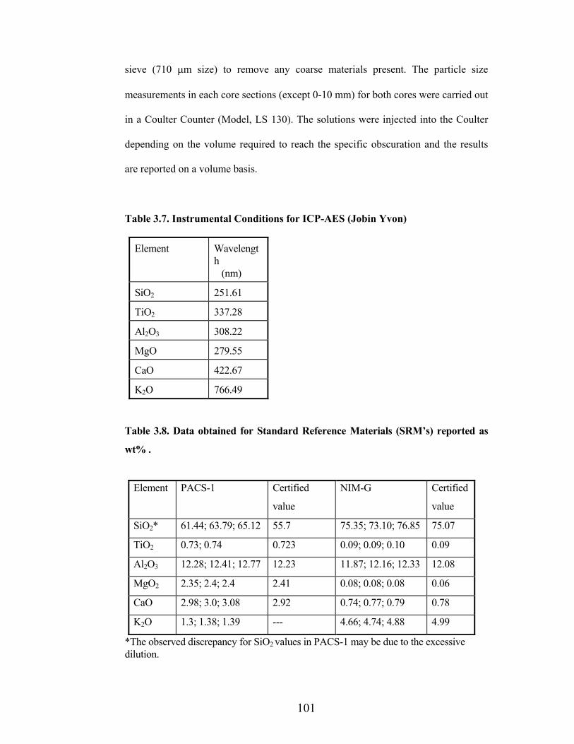
101
sieve (710 m size) to remove any coarse materials present. The particle size
measurements in each core sections (except 0-10 mm) for both cores were carried out
in a Coulter Counter (Model, LS 130). The solutions were injected into the Coulter
depending on the volume required to reach the specific obscuration and the results
are reported on a volume basis.
Table 3.7. Instrumental Conditions for ICP-AES (Jobin Yvon)
Element Wavelength (nm)
SiO2 251.61
TiO2 337.28
Al2O3 308.22
MgO 279.55
CaO 422.67
K2O 766.49
Table 3.8. Data obtained for Standard Reference Materials (SRM’s) reported as
wt% .
Element PACS-1 Certified
value
NIM-G Certified
value
SiO2* 61.44; 63.79; 65.12 55.7 75.35; 73.10; 76.85 75.07
TiO2 0.73; 0.74 0.723 0.09; 0.09; 0.10 0.09
Al2O3 12.28; 12.41; 12.77 12.23 11.87; 12.16; 12.33 12.08
MgO2 2.35; 2.4; 2.4 2.41 0.08; 0.08; 0.08 0.06
CaO 2.98; 3.0; 3.08 2.92 0.74; 0.77; 0.79 0.78
K2O 1.3; 1.38; 1.39 --- 4.66; 4.74; 4.88 4.99
*The observed discrepancy for SiO2 values in PACS-1 may be due to the excessive dilution.

102
3.11. SAMPLING METHODS
3.11.1. Sampling locations
The sampling locations in the Arabian Sea (Oman Margin) are shown in the
Figs.3.8(i&ii).
3.11.2. Sample collection
The samples for this study were collected during Cruise 211 on R.R.S.
Discovery from 8 th October to 12 th November 1994, from the Arabian Basin at a
water depth of approximately 400 m and 3400 m depth. The exact sampling locations of
the multi corer (see Figs. 3.8 i&ii) and the core descriptions are presented in Table 3.9.
Table 3.9. Description of Multi-Corer Sampling Stations
Station No Location Water depth (m)
Core length (mm)
Date taken
12687 # 8 18° 59.33' N 58° 59.09' E
3372 270-290 20/10/94
12687 # 10 18° 59.42' N 59° 00.92' E
3385 310-330 20/10/94
12690 # 1 19° 22.00' N 58° 15.43' E
377 130-150 22/10/94
12692 # 1 19° 21.83' N 58° 15.42' E
372 130-150 22/10/94
12695# 2 19° 22.07' N 58° 15.43' E
382 130-150 22/10/94


104
3.11.3. Sediment core
Sediment cores were collected using a multi-corer (Barnett et al. 1984). Samples
were immediately frozen (-20oC) onboard ship prior to transport to the laboratories.
They were then freeze-dried in the laboratories. The dried samples were stored (-20o C)
prior to analysis. Frozen cores were also collected at this site. Frozen (-20o C) cores were
sectioned as follows 0-5 mm, 5-10 mm, 10-70 mm depth with 10 mm intervals, and
below 70 mm depth with 20 mm intervals.