Embed Size (px)
Citation preview

Chapter 2: Probability
OpenIntro Statistics, 3rd Edition
Slides developed by Mine Cetinkaya-Rundel of OpenIntro.The slides may be copied, edited, and/or shared via the CC BY-SA license.Some images may be included under fair use guidelines (educational purposes).
Defining probability
Random processes
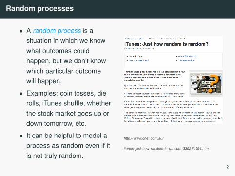
• A random process is asituation in which we knowwhat outcomes couldhappen, but we don’t knowwhich particular outcomewill happen.
• Examples: coin tosses, dierolls, iTunes shuffle, whetherthe stock market goes up ordown tomorrow, etc.
• It can be helpful to model aprocess as random even if itis not truly random.
http:// www.cnet.com.au/
itunes-just-how-random-is-random-339274094.htm
2
Probability
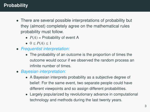
• There are several possible interpretations of probability butthey (almost) completely agree on the mathematical rulesprobability must follow.• P(A) = Probability of event A• 0 ≤ P(A) ≤ 1
• Frequentist interpretation:• The probability of an outcome is the proportion of times the
outcome would occur if we observed the random process aninfinite number of times.
• Bayesian interpretation:• A Bayesian interprets probability as a subjective degree of
belief: For the same event, two separate people could havedifferent viewpoints and so assign different probabilities.
• Largely popularized by revolutionary advance in computationaltechnology and methods during the last twenty years.
3
Probability
• There are several possible interpretations of probability butthey (almost) completely agree on the mathematical rulesprobability must follow.• P(A) = Probability of event A• 0 ≤ P(A) ≤ 1
• Frequentist interpretation:• The probability of an outcome is the proportion of times the
outcome would occur if we observed the random process aninfinite number of times.
• Bayesian interpretation:• A Bayesian interprets probability as a subjective degree of
belief: For the same event, two separate people could havedifferent viewpoints and so assign different probabilities.
• Largely popularized by revolutionary advance in computationaltechnology and methods during the last twenty years.
3
Practice
Which of the following events would you be most surprised by?
(a) exactly 3 heads in 10 coin flips
(b) exactly 3 heads in 100 coin flips
(c) exactly 3 heads in 1000 coin flips
4
Practice
Which of the following events would you be most surprised by?
(a) exactly 3 heads in 10 coin flips
(b) exactly 3 heads in 100 coin flips
(c) exactly 3 heads in 1000 coin flips
4

Law of large numbers
Law of large numbers states that as more observations arecollected, the proportion of occurrences with a particular outcome,pn, converges to the probability of that outcome, p.
5
Law of large numbers (cont.)
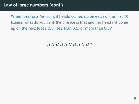
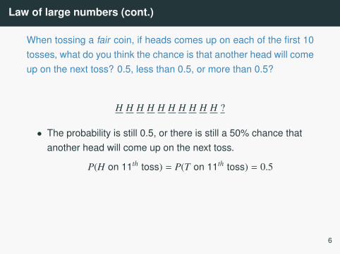
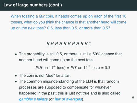
When tossing a fair coin, if heads comes up on each of the first 10tosses, what do you think the chance is that another head will comeup on the next toss? 0.5, less than 0.5, or more than 0.5?
H H H H H H H H H H ?
• The probability is still 0.5, or there is still a 50% chance thatanother head will come up on the next toss.
P(H on 11th toss) = P(T on 11th toss) = 0.5
• The coin is not “due” for a tail.• The common misunderstanding of the LLN is that random
processes are supposed to compensate for whateverhappened in the past; this is just not true and is also calledgambler’s fallacy (or law of averages).
6
Law of large numbers (cont.)
When tossing a fair coin, if heads comes up on each of the first 10tosses, what do you think the chance is that another head will comeup on the next toss? 0.5, less than 0.5, or more than 0.5?
H H H H H H H H H H ?
• The probability is still 0.5, or there is still a 50% chance thatanother head will come up on the next toss.
P(H on 11th toss) = P(T on 11th toss) = 0.5
• The coin is not “due” for a tail.• The common misunderstanding of the LLN is that random
processes are supposed to compensate for whateverhappened in the past; this is just not true and is also calledgambler’s fallacy (or law of averages).
6

Law of large numbers (cont.)
When tossing a fair coin, if heads comes up on each of the first 10tosses, what do you think the chance is that another head will comeup on the next toss? 0.5, less than 0.5, or more than 0.5?
H H H H H H H H H H ?
• The probability is still 0.5, or there is still a 50% chance thatanother head will come up on the next toss.
P(H on 11th toss) = P(T on 11th toss) = 0.5
• The coin is not “due” for a tail.
• The common misunderstanding of the LLN is that randomprocesses are supposed to compensate for whateverhappened in the past; this is just not true and is also calledgambler’s fallacy (or law of averages).
6
Law of large numbers (cont.)
When tossing a fair coin, if heads comes up on each of the first 10tosses, what do you think the chance is that another head will comeup on the next toss? 0.5, less than 0.5, or more than 0.5?
H H H H H H H H H H ?
• The probability is still 0.5, or there is still a 50% chance thatanother head will come up on the next toss.
P(H on 11th toss) = P(T on 11th toss) = 0.5
• The coin is not “due” for a tail.• The common misunderstanding of the LLN is that random
processes are supposed to compensate for whateverhappened in the past; this is just not true and is also calledgambler’s fallacy (or law of averages). 6
Disjoint and non-disjoint outcomes
Disjoint (mutually exclusive) outcomes: Cannot happen at thesame time.
• The outcome of a single coin toss cannot be a head and a tail.
• A student both cannot fail and pass a class.
• A single card drawn from a deck cannot be an ace and aqueen.
Non-disjoint outcomes: Can happen at the same time.
• A student can get an A in Stats and A in Econ in the samesemester.
7
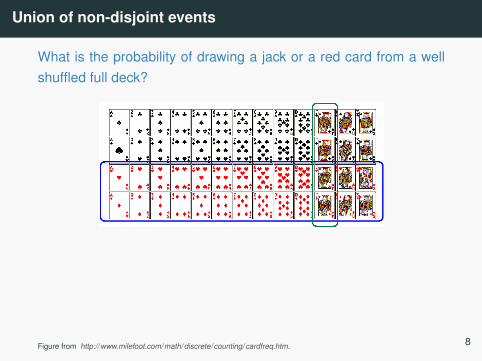
Union of non-disjoint events
What is the probability of drawing a jack or a red card from a wellshuffled full deck?
P(jack or red) = P(jack) + P(red) − P(jack and red)
=452+
2652−
252=
2852
Figure from http:// www.milefoot.com/ math/ discrete/ counting/ cardfreq.htm. 8
Union of non-disjoint events
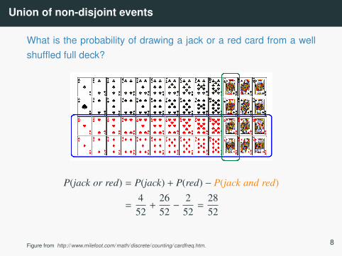
What is the probability of drawing a jack or a red card from a wellshuffled full deck?
P(jack or red) = P(jack) + P(red) − P(jack and red)
=452+
2652−
252=
2852
Figure from http:// www.milefoot.com/ math/ discrete/ counting/ cardfreq.htm. 8
Practice
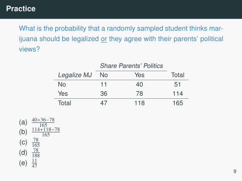
What is the probability that a randomly sampled student thinks mar-ijuana should be legalized or they agree with their parents’ politicalviews?
Share Parents’ PoliticsLegalize MJ No Yes TotalNo 11 40 51Yes 36 78 114Total 47 118 165
(a) 40+36−78165
(b) 114+118−78165
(c) 78165
(d) 78188
(e) 1147
9
Practice
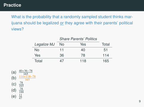
What is the probability that a randomly sampled student thinks mar-ijuana should be legalized or they agree with their parents’ politicalviews?
Share Parents’ PoliticsLegalize MJ No Yes TotalNo 11 40 51Yes 36 78 114Total 47 118 165
(a) 40+36−78165
(b) 114+118−78165
(c) 78165
(d) 78188
(e) 1147
9
Recap
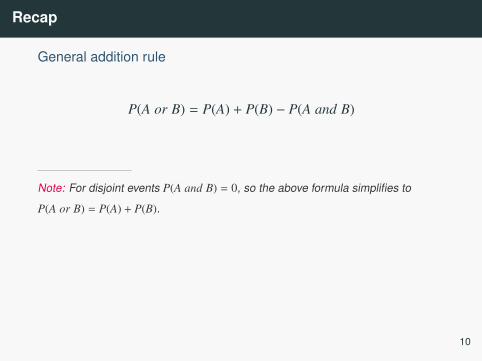
General addition rule
P(A or B) = P(A) + P(B) − P(A and B)
Note: For disjoint events P(A and B) = 0, so the above formula simplifies to
P(A or B) = P(A) + P(B).
10
Probability distributions
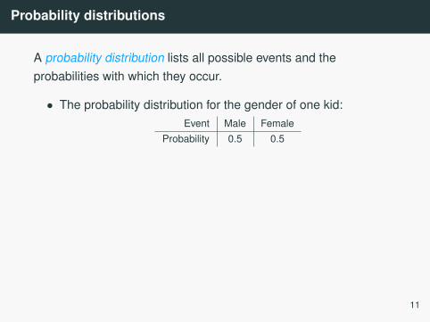
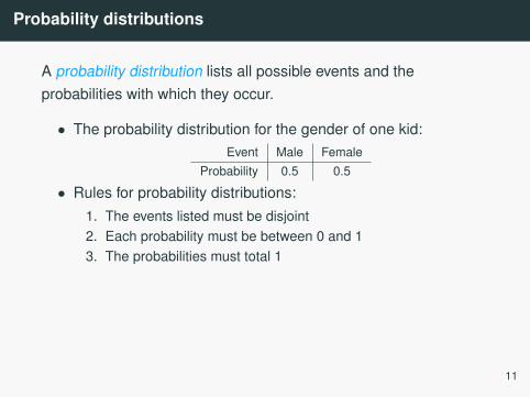
A probability distribution lists all possible events and theprobabilities with which they occur.
• The probability distribution for the gender of one kid:Event Male Female
Probability 0.5 0.5
• Rules for probability distributions:1. The events listed must be disjoint2. Each probability must be between 0 and 13. The probabilities must total 1
• The probability distribution for the genders of two kids:
11
Probability distributions
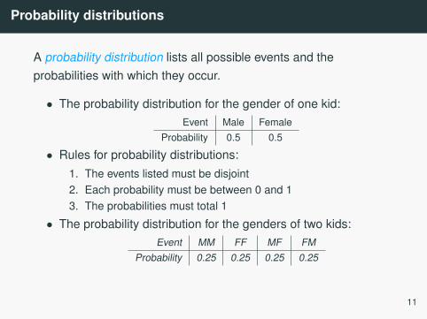
A probability distribution lists all possible events and theprobabilities with which they occur.
• The probability distribution for the gender of one kid:Event Male Female
Probability 0.5 0.5
• Rules for probability distributions:1. The events listed must be disjoint2. Each probability must be between 0 and 13. The probabilities must total 1
• The probability distribution for the genders of two kids:Event MM FF MF FM
Probability 0.25 0.25 0.25 0.25
11
Probability distributions
A probability distribution lists all possible events and theprobabilities with which they occur.
• The probability distribution for the gender of one kid:Event Male Female
Probability 0.5 0.5
• Rules for probability distributions:1. The events listed must be disjoint2. Each probability must be between 0 and 13. The probabilities must total 1
• The probability distribution for the genders of two kids:Event MM FF MF FM
Probability 0.25 0.25 0.25 0.25
11
Practice
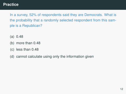
In a survey, 52% of respondents said they are Democrats. What isthe probability that a randomly selected respondent from this sam-ple is a Republican?
(a) 0.48
(b) more than 0.48
(c) less than 0.48
(d) cannot calculate using only the information given
12
Practice
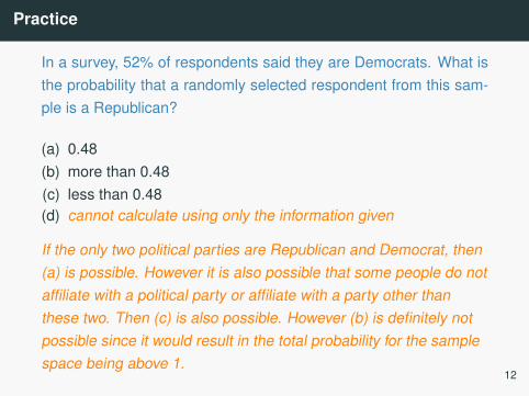
In a survey, 52% of respondents said they are Democrats. What isthe probability that a randomly selected respondent from this sam-ple is a Republican?
(a) 0.48(b) more than 0.48(c) less than 0.48(d) cannot calculate using only the information given
If the only two political parties are Republican and Democrat, then(a) is possible. However it is also possible that some people do notaffiliate with a political party or affiliate with a party other thanthese two. Then (c) is also possible. However (b) is definitely notpossible since it would result in the total probability for the samplespace being above 1.
12
Sample space and complements
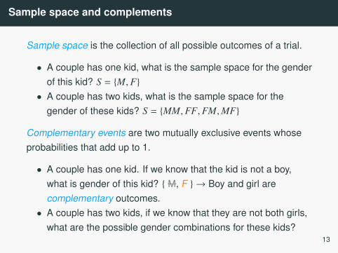
Sample space is the collection of all possible outcomes of a trial.
• A couple has one kid, what is the sample space for the genderof this kid? S = {M,F}
• A couple has two kids, what is the sample space for thegender of these kids?
S = {MM,FF,FM,MF}
Complementary events are two mutually exclusive events whoseprobabilities that add up to 1.
• A couple has one kid. If we know that the kid is not a boy,what is gender of this kid? { M, F } → Boy and girl arecomplementary outcomes.
• A couple has two kids, if we know that they are not both girls,what are the possible gender combinations for these kids? {MM, FF, FM, MF }
13
Sample space and complements
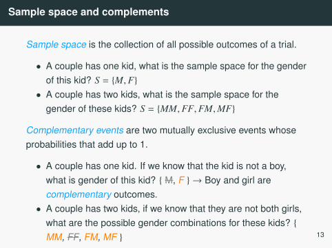
Sample space is the collection of all possible outcomes of a trial.
• A couple has one kid, what is the sample space for the genderof this kid? S = {M,F}
• A couple has two kids, what is the sample space for thegender of these kids? S = {MM,FF,FM,MF}
Complementary events are two mutually exclusive events whoseprobabilities that add up to 1.
• A couple has one kid. If we know that the kid is not a boy,what is gender of this kid? { M, F } → Boy and girl arecomplementary outcomes.
• A couple has two kids, if we know that they are not both girls,what are the possible gender combinations for these kids? {MM, FF, FM, MF }
13
Sample space and complements
Sample space is the collection of all possible outcomes of a trial.
• A couple has one kid, what is the sample space for the genderof this kid? S = {M,F}
• A couple has two kids, what is the sample space for thegender of these kids? S = {MM,FF,FM,MF}
Complementary events are two mutually exclusive events whoseprobabilities that add up to 1.
• A couple has one kid. If we know that the kid is not a boy,what is gender of this kid? { M, F } → Boy and girl arecomplementary outcomes.
• A couple has two kids, if we know that they are not both girls,what are the possible gender combinations for these kids?
{
MM, FF, FM, MF }
13
Sample space and complements
Sample space is the collection of all possible outcomes of a trial.
• A couple has one kid, what is the sample space for the genderof this kid? S = {M,F}
• A couple has two kids, what is the sample space for thegender of these kids? S = {MM,FF,FM,MF}
Complementary events are two mutually exclusive events whoseprobabilities that add up to 1.
• A couple has one kid. If we know that the kid is not a boy,what is gender of this kid? { M, F } → Boy and girl arecomplementary outcomes.
• A couple has two kids, if we know that they are not both girls,what are the possible gender combinations for these kids? {MM, FF, FM, MF } 13
Independence
Two processes are independent if knowing the outcome of oneprovides no useful information about the outcome of the other.
• Knowing that the coin landed on a head on the first tossdoes not provide any useful information for determining whatthe coin will land on in the second toss. → Outcomes of twotosses of a coin are independent.
• Knowing that the first card drawn from a deck is an ace doesprovide useful information for determining the probability ofdrawing an ace in the second draw. → Outcomes of two drawsfrom a deck of cards (without replacement) are dependent.
14

Practice
Between January 9-12, 2013, SurveyUSA interviewed a random sampleof 500 NC residents asking them whether they think widespread gun own-ership protects law abiding citizens from crime, or makes society moredangerous. 58% of all respondents said it protects citizens. 67% of Whiterespondents, 28% of Black respondents, and 64% of Hispanic respon-dents shared this view. Which of the below is true?
Opinion on gun ownership and race ethnicity are most likely
(a) complementary(b) mutually exclusive(c) independent(d) dependent(e) disjoint
http:// www.surveyusa.com/ client/ PollReport.aspx?g=a5f460ef-bba9-484b-8579-1101ea26421b
15
Checking for independence
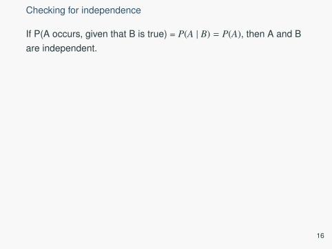
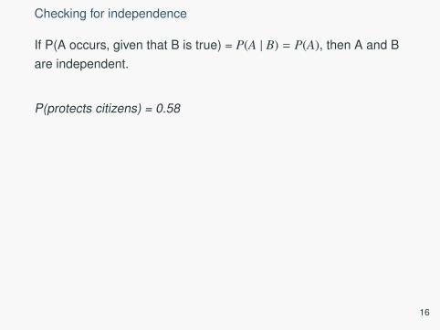
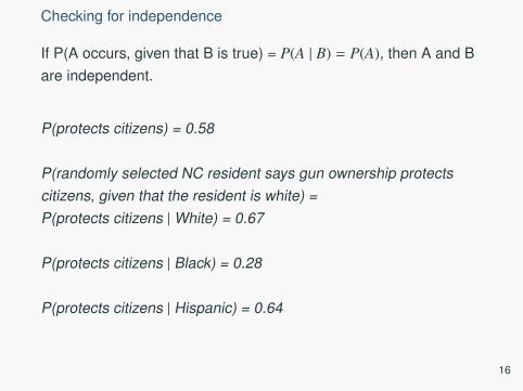
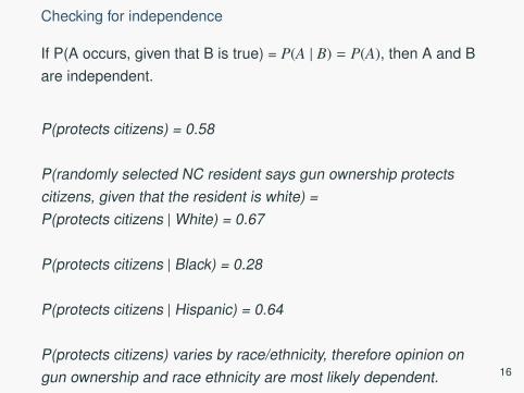
If P(A occurs, given that B is true) = P(A | B) = P(A), then A and Bare independent.
P(protects citizens) = 0.58
P(randomly selected NC resident says gun ownership protectscitizens, given that the resident is white) =P(protects citizens |White) = 0.67
P(protects citizens | Black) = 0.28
P(protects citizens | Hispanic) = 0.64
P(protects citizens) varies by race/ethnicity, therefore opinion ongun ownership and race ethnicity are most likely dependent.
16
Checking for independence
If P(A occurs, given that B is true) = P(A | B) = P(A), then A and Bare independent.
P(protects citizens) = 0.58
P(randomly selected NC resident says gun ownership protectscitizens, given that the resident is white) =P(protects citizens |White) = 0.67
P(protects citizens | Black) = 0.28
P(protects citizens | Hispanic) = 0.64
P(protects citizens) varies by race/ethnicity, therefore opinion ongun ownership and race ethnicity are most likely dependent. 16

Determining dependence based on sample data
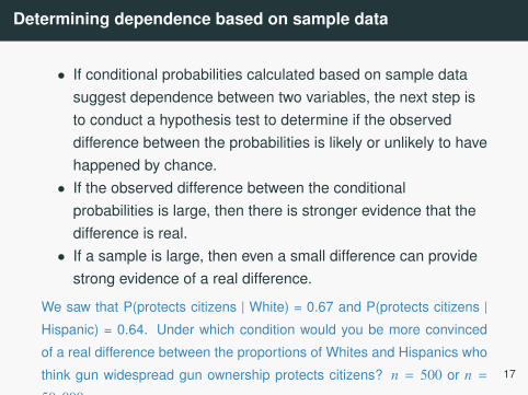
• If conditional probabilities calculated based on sample datasuggest dependence between two variables, the next step isto conduct a hypothesis test to determine if the observeddifference between the probabilities is likely or unlikely to havehappened by chance.
• If the observed difference between the conditionalprobabilities is large, then there is stronger evidence that thedifference is real.
• If a sample is large, then even a small difference can providestrong evidence of a real difference.
We saw that P(protects citizens | White) = 0.67 and P(protects citizens |
Hispanic) = 0.64. Under which condition would you be more convinced
of a real difference between the proportions of Whites and Hispanics who
think gun widespread gun ownership protects citizens? n = 500 or n =
50, 000
n = 50, 000
17
Determining dependence based on sample data
• If conditional probabilities calculated based on sample datasuggest dependence between two variables, the next step isto conduct a hypothesis test to determine if the observeddifference between the probabilities is likely or unlikely to havehappened by chance.
• If the observed difference between the conditionalprobabilities is large, then there is stronger evidence that thedifference is real.
• If a sample is large, then even a small difference can providestrong evidence of a real difference.
We saw that P(protects citizens | White) = 0.67 and P(protects citizens |
Hispanic) = 0.64. Under which condition would you be more convinced
of a real difference between the proportions of Whites and Hispanics who
think gun widespread gun ownership protects citizens? n = 500 or n =
50, 000
n = 50, 000
17
Product rule for independent events
P(A and B) = P(A) × P(B)
Or more generally, P(A1 and · · · and Ak) = P(A1) × · · · × P(Ak)
You toss a coin twice, what is the probability of getting two tails in arow?
P(T on the first toss) × P(T on the second toss) =12×
12=
14
18
Product rule for independent events
P(A and B) = P(A) × P(B)
Or more generally, P(A1 and · · · and Ak) = P(A1) × · · · × P(Ak)
You toss a coin twice, what is the probability of getting two tails in arow?
P(T on the first toss) × P(T on the second toss) =12×
12=
14
18

Product rule for independent events
P(A and B) = P(A) × P(B)
Or more generally, P(A1 and · · · and Ak) = P(A1) × · · · × P(Ak)
You toss a coin twice, what is the probability of getting two tails in arow?
P(T on the first toss) × P(T on the second toss) =12×
12=
14
18

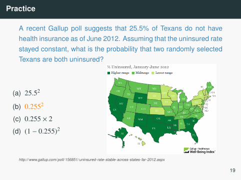
Practice
A recent Gallup poll suggests that 25.5% of Texans do not havehealth insurance as of June 2012. Assuming that the uninsured ratestayed constant, what is the probability that two randomly selectedTexans are both uninsured?
(a) 25.52
(b) 0.2552
(c) 0.255 × 2
(d) (1 − 0.255)2
http:// www.gallup.com/ poll/ 156851/ uninsured-rate-stable-across-states-far-2012.aspx
19
Disjoint vs. complementary
Do the sum of probabilities of two disjoint events always add up to1?
Not necessarily, there may be more than 2 events in the samplespace, e.g. party affiliation.
Do the sum of probabilities of two complementary events alwaysadd up to 1?
Yes, that’s the definition of complementary, e.g. heads and tails.
20
Putting everything together...
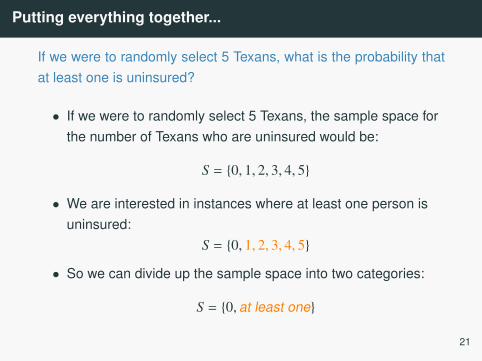
If we were to randomly select 5 Texans, what is the probability thatat least one is uninsured?
• If we were to randomly select 5 Texans, the sample space forthe number of Texans who are uninsured would be:
S = {0, 1, 2, 3, 4, 5}
• We are interested in instances where at least one person isuninsured:
S = {0, 1, 2, 3, 4, 5}
• So we can divide up the sample space into two categories:
S = {0, at least one}
21
Putting everything together...
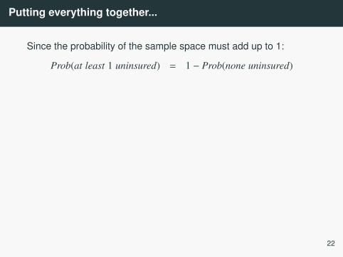
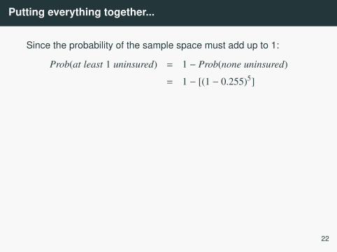
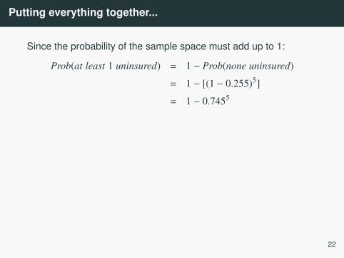
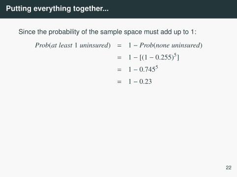
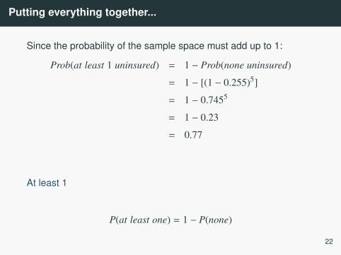
Since the probability of the sample space must add up to 1:
Prob(at least 1 uninsured) = 1 − Prob(none uninsured)
= 1 − [(1 − 0.255)5]
= 1 − 0.7455
= 1 − 0.23
= 0.77
At least 1
P(at least one) = 1 − P(none)
22
Putting everything together...
Since the probability of the sample space must add up to 1:
Prob(at least 1 uninsured) = 1 − Prob(none uninsured)
= 1 − [(1 − 0.255)5]
= 1 − 0.7455
= 1 − 0.23
= 0.77
At least 1
P(at least one) = 1 − P(none)
22
Putting everything together...
Since the probability of the sample space must add up to 1:
Prob(at least 1 uninsured) = 1 − Prob(none uninsured)
= 1 − [(1 − 0.255)5]
= 1 − 0.7455
= 1 − 0.23
= 0.77
At least 1
P(at least one) = 1 − P(none)
22
Putting everything together...
Since the probability of the sample space must add up to 1:
Prob(at least 1 uninsured) = 1 − Prob(none uninsured)
= 1 − [(1 − 0.255)5]
= 1 − 0.7455
= 1 − 0.23
= 0.77
At least 1
P(at least one) = 1 − P(none)
22
Putting everything together...
Since the probability of the sample space must add up to 1:
Prob(at least 1 uninsured) = 1 − Prob(none uninsured)
= 1 − [(1 − 0.255)5]
= 1 − 0.7455
= 1 − 0.23
= 0.77
At least 1
P(at least one) = 1 − P(none)
22
Practice
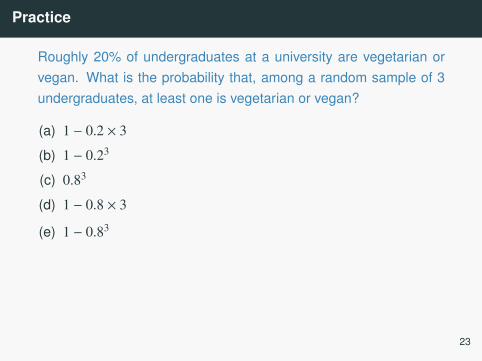
Roughly 20% of undergraduates at a university are vegetarian orvegan. What is the probability that, among a random sample of 3undergraduates, at least one is vegetarian or vegan?
(a) 1 − 0.2 × 3
(b) 1 − 0.23
(c) 0.83
(d) 1 − 0.8 × 3
(e) 1 − 0.83
23
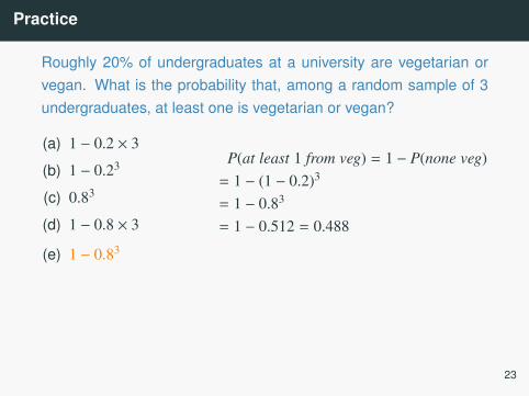
Practice
Roughly 20% of undergraduates at a university are vegetarian orvegan. What is the probability that, among a random sample of 3undergraduates, at least one is vegetarian or vegan?
(a) 1 − 0.2 × 3
(b) 1 − 0.23
(c) 0.83
(d) 1 − 0.8 × 3
(e) 1 − 0.83
P(at least 1 from veg) = 1 − P(none veg)= 1 − (1 − 0.2)3
= 1 − 0.83
= 1 − 0.512 = 0.488
23
Conditional probability
Relapse
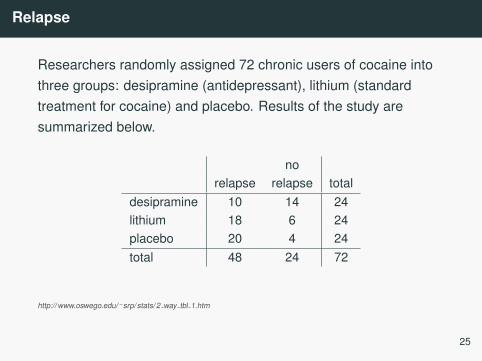
Researchers randomly assigned 72 chronic users of cocaine intothree groups: desipramine (antidepressant), lithium (standardtreatment for cocaine) and placebo. Results of the study aresummarized below.
norelapse relapse total
desipramine 10 14 24lithium 18 6 24placebo 20 4 24total 48 24 72
http:// www.oswego.edu/∼srp/ stats/ 2 way tbl 1.htm
25
Marginal probability
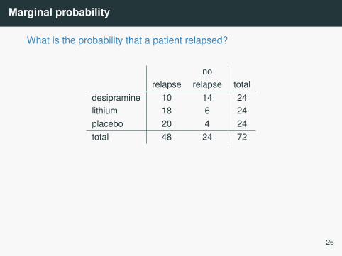
What is the probability that a patient relapsed?
norelapse relapse total
desipramine 10 14 24lithium 18 6 24placebo 20 4 24total 48 24 72
P(relapsed) = 4872 ≈ 0.67
26

Marginal probability
What is the probability that a patient relapsed?
norelapse relapse total
desipramine 10 14 24lithium 18 6 24placebo 20 4 24total 48 24 72
P(relapsed) = 4872 ≈ 0.67
26
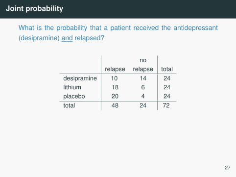
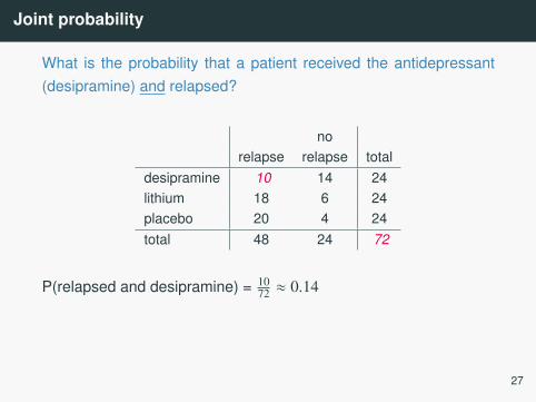
Joint probability
What is the probability that a patient received the antidepressant(desipramine) and relapsed?
norelapse relapse total
desipramine 10 14 24lithium 18 6 24placebo 20 4 24total 48 24 72
P(relapsed and desipramine) = 1072 ≈ 0.14
27
Joint probability
What is the probability that a patient received the antidepressant(desipramine) and relapsed?
norelapse relapse total
desipramine 10 14 24lithium 18 6 24placebo 20 4 24total 48 24 72
P(relapsed and desipramine) = 1072 ≈ 0.14
27
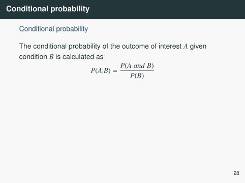
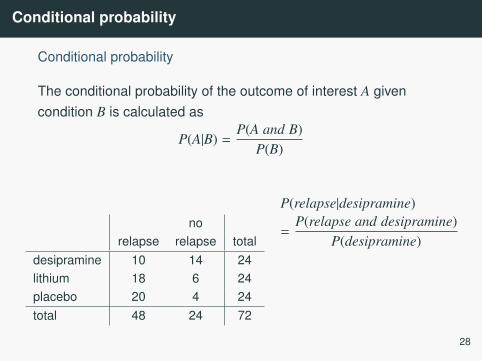
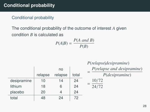
Conditional probability
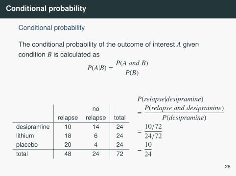
Conditional probability
The conditional probability of the outcome of interest A givencondition B is calculated as
P(A|B) =P(A and B)
P(B)
norelapse relapse total
desipramine 10 14 24lithium 18 6 24placebo 20 4 24total 48 24 72
P(relapse|desipramine)
=P(relapse and desipramine)
P(desipramine)
=10/7224/72
=1024
= 0.42
28
Conditional probability
Conditional probability
The conditional probability of the outcome of interest A givencondition B is calculated as
P(A|B) =P(A and B)
P(B)
norelapse relapse total
desipramine 10 14 24lithium 18 6 24placebo 20 4 24total 48 24 72
P(relapse|desipramine)
=P(relapse and desipramine)
P(desipramine)
=10/7224/72
=1024
= 0.42
28
Conditional probability
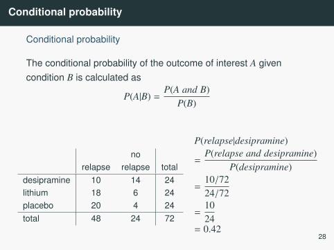
Conditional probability
The conditional probability of the outcome of interest A givencondition B is calculated as
P(A|B) =P(A and B)
P(B)
norelapse relapse total
desipramine 10 14 24lithium 18 6 24placebo 20 4 24total 48 24 72
P(relapse|desipramine)
=P(relapse and desipramine)
P(desipramine)
=10/7224/72
=1024
= 0.4228
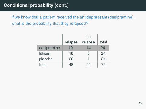
Conditional probability (cont.)
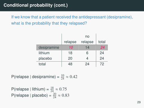
If we know that a patient received the antidepressant (desipramine),what is the probability that they relapsed?
norelapse relapse total
desipramine 10 14 24lithium 18 6 24placebo 20 4 24total 48 24 72
P(relapse | desipramine) = 1024 ≈ 0.42
P(relapse | lithium) = 1824 ≈ 0.75
P(relapse | placebo) = 2024 ≈ 0.83
29
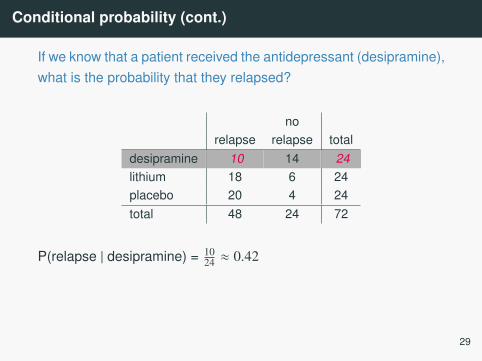
Conditional probability (cont.)
If we know that a patient received the antidepressant (desipramine),what is the probability that they relapsed?
norelapse relapse total
desipramine 10 14 24lithium 18 6 24placebo 20 4 24total 48 24 72
P(relapse | desipramine) = 1024 ≈ 0.42
P(relapse | lithium) = 1824 ≈ 0.75
P(relapse | placebo) = 2024 ≈ 0.83
29
Conditional probability (cont.)
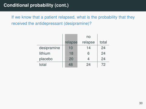
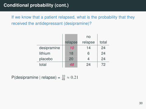
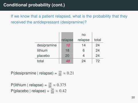
If we know that a patient relapsed, what is the probability that theyreceived the antidepressant (desipramine)?
norelapse relapse total
desipramine 10 14 24lithium 18 6 24placebo 20 4 24total 48 24 72
P(desipramine | relapse) = 1048 ≈ 0.21
P(lithium | relapse) = 1848 ≈ 0.375
P(placebo | relapse) = 2048 ≈ 0.42
30
Conditional probability (cont.)
If we know that a patient relapsed, what is the probability that theyreceived the antidepressant (desipramine)?
norelapse relapse total
desipramine 10 14 24lithium 18 6 24placebo 20 4 24total 48 24 72
P(desipramine | relapse) = 1048 ≈ 0.21
P(lithium | relapse) = 1848 ≈ 0.375
P(placebo | relapse) = 2048 ≈ 0.42
30

General multiplication rule
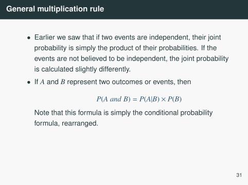
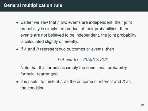
• Earlier we saw that if two events are independent, their jointprobability is simply the product of their probabilities. If theevents are not believed to be independent, the joint probabilityis calculated slightly differently.
• If A and B represent two outcomes or events, then
P(A and B) = P(A|B) × P(B)
Note that this formula is simply the conditional probabilityformula, rearranged.
• It is useful to think of A as the outcome of interest and B asthe condition.
31
General multiplication rule
• Earlier we saw that if two events are independent, their jointprobability is simply the product of their probabilities. If theevents are not believed to be independent, the joint probabilityis calculated slightly differently.
• If A and B represent two outcomes or events, then
P(A and B) = P(A|B) × P(B)
Note that this formula is simply the conditional probabilityformula, rearranged.
• It is useful to think of A as the outcome of interest and B asthe condition.
31
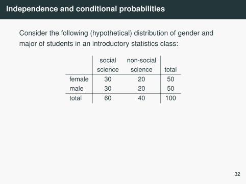
Independence and conditional probabilities
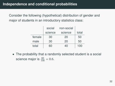
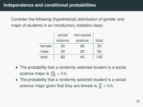
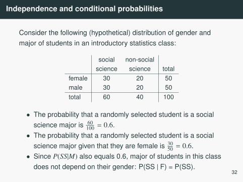
Consider the following (hypothetical) distribution of gender andmajor of students in an introductory statistics class:
social non-socialscience science total
female 30 20 50male 30 20 50total 60 40 100
• The probability that a randomly selected student is a socialscience major is 60
100 = 0.6.• The probability that a randomly selected student is a social
science major given that they are female is 3050 = 0.6.
• Since P(SS|M) also equals 0.6, major of students in this classdoes not depend on their gender: P(SS | F) = P(SS).
32
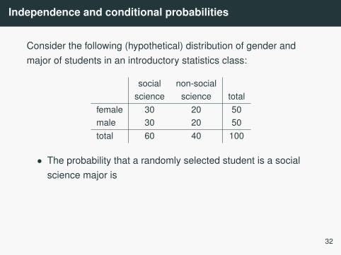
Independence and conditional probabilities
Consider the following (hypothetical) distribution of gender andmajor of students in an introductory statistics class:
social non-socialscience science total
female 30 20 50male 30 20 50total 60 40 100
• The probability that a randomly selected student is a socialscience major is
60100 = 0.6.
• The probability that a randomly selected student is a socialscience major given that they are female is 30
50 = 0.6.• Since P(SS|M) also equals 0.6, major of students in this class
does not depend on their gender: P(SS | F) = P(SS).
32
Independence and conditional probabilities
Consider the following (hypothetical) distribution of gender andmajor of students in an introductory statistics class:
social non-socialscience science total
female 30 20 50male 30 20 50total 60 40 100
• The probability that a randomly selected student is a socialscience major is 60
100 = 0.6.
• The probability that a randomly selected student is a socialscience major given that they are female is 30
50 = 0.6.• Since P(SS|M) also equals 0.6, major of students in this class
does not depend on their gender: P(SS | F) = P(SS).
32

Independence and conditional probabilities
Consider the following (hypothetical) distribution of gender andmajor of students in an introductory statistics class:
social non-socialscience science total
female 30 20 50male 30 20 50total 60 40 100
• The probability that a randomly selected student is a socialscience major is 60
100 = 0.6.• The probability that a randomly selected student is a social
science major given that they are female is
3050 = 0.6.
• Since P(SS|M) also equals 0.6, major of students in this classdoes not depend on their gender: P(SS | F) = P(SS).
32
Independence and conditional probabilities
Consider the following (hypothetical) distribution of gender andmajor of students in an introductory statistics class:
social non-socialscience science total
female 30 20 50male 30 20 50total 60 40 100
• The probability that a randomly selected student is a socialscience major is 60
100 = 0.6.• The probability that a randomly selected student is a social
science major given that they are female is 3050 = 0.6.
• Since P(SS|M) also equals 0.6, major of students in this classdoes not depend on their gender: P(SS | F) = P(SS).
32

Independence and conditional probabilities (cont.)
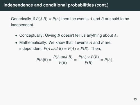
Generically, if P(A|B) = P(A) then the events A and B are said to beindependent.
• Conceptually: Giving B doesn’t tell us anything about A.
• Mathematically: We know that if events A and B areindependent, P(A and B) = P(A) × P(B). Then,
P(A|B) =P(A and B)
P(B)=
P(A) × P(B)P(B)
= P(A)
33
Independence and conditional probabilities (cont.)
Generically, if P(A|B) = P(A) then the events A and B are said to beindependent.
• Conceptually: Giving B doesn’t tell us anything about A.
• Mathematically: We know that if events A and B areindependent, P(A and B) = P(A) × P(B). Then,
P(A|B) =P(A and B)
P(B)=
P(A) × P(B)P(B)
= P(A)
33

Breast cancer screening
• American Cancer Society estimates that about 1.7% ofwomen have breast cancer.http:// www.cancer.org/ cancer/ cancerbasics/ cancer-prevalence
• Susan G. Komen For The Cure Foundation states thatmammography correctly identifies about 78% of women whotruly have breast cancer.http:
// ww5.komen.org/ BreastCancer/ AccuracyofMammograms.html
• An article published in 2003 suggests that up to 10% of allmammograms result in false positives for patients who do nothave cancer.http:// www.ncbi.nlm.nih.gov/ pmc/ articles/ PMC1360940
Note: These percentages are approximate, and very difficult to estimate.34
Inverting probabilities
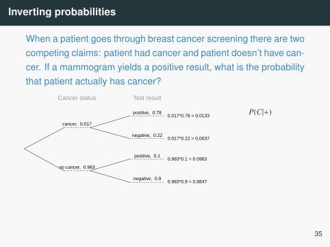
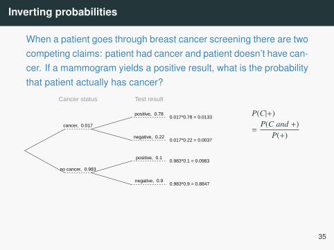
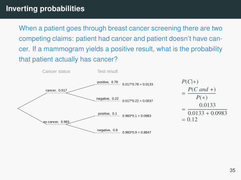
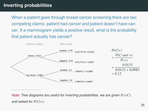
When a patient goes through breast cancer screening there are twocompeting claims: patient had cancer and patient doesn’t have can-cer. If a mammogram yields a positive result, what is the probabilitythat patient actually has cancer?
Cancer status Test result
cancer, 0.017
positive, 0.780.017*0.78 = 0.0133
negative, 0.220.017*0.22 = 0.0037
no cancer, 0.983
positive, 0.10.983*0.1 = 0.0983
negative, 0.90.983*0.9 = 0.8847
P(C|+)
=P(C and +)
P(+)
=0.0133
0.0133 + 0.0983= 0.12
Note: Tree diagrams are useful for inverting probabilities: we are given P(+|C)
and asked for P(C|+).
35

Inverting probabilities
When a patient goes through breast cancer screening there are twocompeting claims: patient had cancer and patient doesn’t have can-cer. If a mammogram yields a positive result, what is the probabilitythat patient actually has cancer?
Cancer status Test result
cancer, 0.017
positive, 0.780.017*0.78 = 0.0133
negative, 0.220.017*0.22 = 0.0037
no cancer, 0.983
positive, 0.10.983*0.1 = 0.0983
negative, 0.90.983*0.9 = 0.8847
P(C|+)
=P(C and +)
P(+)
=0.0133
0.0133 + 0.0983= 0.12
Note: Tree diagrams are useful for inverting probabilities: we are given P(+|C)
and asked for P(C|+).
35

Inverting probabilities
When a patient goes through breast cancer screening there are twocompeting claims: patient had cancer and patient doesn’t have can-cer. If a mammogram yields a positive result, what is the probabilitythat patient actually has cancer?
Cancer status Test result
cancer, 0.017
positive, 0.780.017*0.78 = 0.0133
negative, 0.220.017*0.22 = 0.0037
no cancer, 0.983
positive, 0.10.983*0.1 = 0.0983
negative, 0.90.983*0.9 = 0.8847
P(C|+)
=P(C and +)
P(+)
=0.0133
0.0133 + 0.0983
= 0.12
Note: Tree diagrams are useful for inverting probabilities: we are given P(+|C)
and asked for P(C|+).
35
Inverting probabilities
When a patient goes through breast cancer screening there are twocompeting claims: patient had cancer and patient doesn’t have can-cer. If a mammogram yields a positive result, what is the probabilitythat patient actually has cancer?
Cancer status Test result
cancer, 0.017
positive, 0.780.017*0.78 = 0.0133
negative, 0.220.017*0.22 = 0.0037
no cancer, 0.983
positive, 0.10.983*0.1 = 0.0983
negative, 0.90.983*0.9 = 0.8847
P(C|+)
=P(C and +)
P(+)
=0.0133
0.0133 + 0.0983= 0.12
Note: Tree diagrams are useful for inverting probabilities: we are given P(+|C)
and asked for P(C|+).
35
Inverting probabilities
When a patient goes through breast cancer screening there are twocompeting claims: patient had cancer and patient doesn’t have can-cer. If a mammogram yields a positive result, what is the probabilitythat patient actually has cancer?
Cancer status Test result
cancer, 0.017
positive, 0.780.017*0.78 = 0.0133
negative, 0.220.017*0.22 = 0.0037
no cancer, 0.983
positive, 0.10.983*0.1 = 0.0983
negative, 0.90.983*0.9 = 0.8847
P(C|+)
=P(C and +)
P(+)
=0.0133
0.0133 + 0.0983= 0.12
Note: Tree diagrams are useful for inverting probabilities: we are given P(+|C)
and asked for P(C|+).35
Practice
Suppose a woman who gets tested once and obtains a positiveresult wants to get tested again. In the second test, what should weassume to be the probability of this specific woman having cancer?
(a) 0.017
(b) 0.12
(c) 0.0133
(d) 0.88
36

Practice
Suppose a woman who gets tested once and obtains a positiveresult wants to get tested again. In the second test, what should weassume to be the probability of this specific woman having cancer?
(a) 0.017
(b) 0.12
(c) 0.0133
(d) 0.88
36
Practice
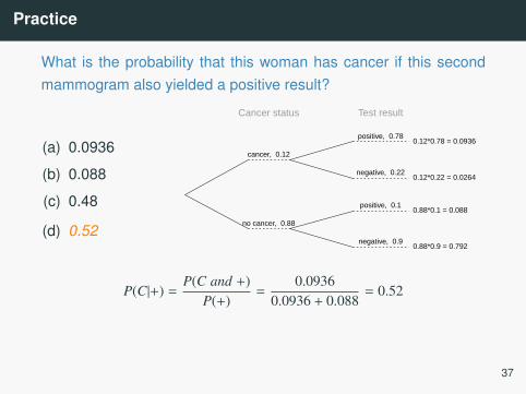
What is the probability that this woman has cancer if this secondmammogram also yielded a positive result?
(a) 0.0936
(b) 0.088
(c) 0.48
(d) 0.52
37

Practice
What is the probability that this woman has cancer if this secondmammogram also yielded a positive result?
(a) 0.0936
(b) 0.088
(c) 0.48
(d) 0.52
Cancer status Test result
cancer, 0.12
positive, 0.780.12*0.78 = 0.0936
negative, 0.220.12*0.22 = 0.0264
no cancer, 0.88
positive, 0.10.88*0.1 = 0.088
negative, 0.90.88*0.9 = 0.792
37
Practice
What is the probability that this woman has cancer if this secondmammogram also yielded a positive result?
(a) 0.0936
(b) 0.088
(c) 0.48
(d) 0.52
Cancer status Test result
cancer, 0.12
positive, 0.780.12*0.78 = 0.0936
negative, 0.220.12*0.22 = 0.0264
no cancer, 0.88
positive, 0.10.88*0.1 = 0.088
negative, 0.90.88*0.9 = 0.792
P(C|+) =P(C and +)
P(+)=
0.09360.0936 + 0.088
= 0.52
37
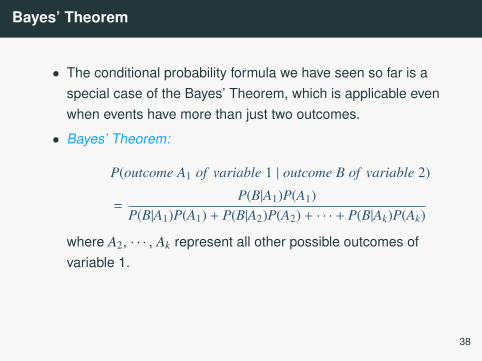
Bayes’ Theorem
• The conditional probability formula we have seen so far is aspecial case of the Bayes’ Theorem, which is applicable evenwhen events have more than just two outcomes.
• Bayes’ Theorem:
P(outcome A1 of variable 1 | outcome B of variable 2)
=P(B|A1)P(A1)
P(B|A1)P(A1) + P(B|A2)P(A2) + · · · + P(B|Ak)P(Ak)
where A2, · · · , Ak represent all other possible outcomes ofvariable 1.
38
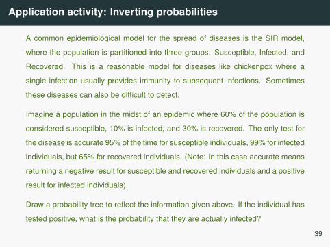
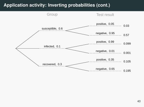
Application activity: Inverting probabilities
A common epidemiological model for the spread of diseases is the SIR model,
where the population is partitioned into three groups: Susceptible, Infected, and
Recovered. This is a reasonable model for diseases like chickenpox where a
single infection usually provides immunity to subsequent infections. Sometimes
these diseases can also be difficult to detect.
Imagine a population in the midst of an epidemic where 60% of the population is
considered susceptible, 10% is infected, and 30% is recovered. The only test for
the disease is accurate 95% of the time for susceptible individuals, 99% for infected
individuals, but 65% for recovered individuals. (Note: In this case accurate means
returning a negative result for susceptible and recovered individuals and a positive
result for infected individuals).
Draw a probability tree to reflect the information given above. If the individual has
tested positive, what is the probability that they are actually infected?
39
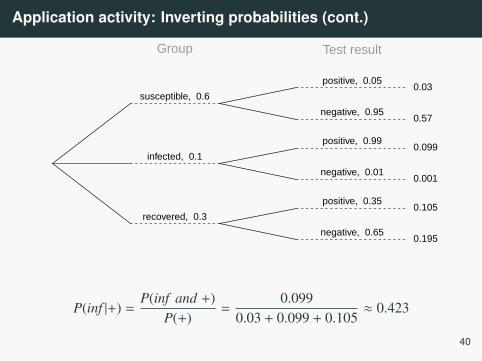
Application activity: Inverting probabilities (cont.)
Group Test result
susceptible, 0.6
positive, 0.050.03
negative, 0.950.57
infected, 0.1
positive, 0.990.099
negative, 0.010.001
recovered, 0.3
positive, 0.350.105
negative, 0.650.195
P(inf |+) =P(inf and +)
P(+)=
0.0990.03 + 0.099 + 0.105
≈ 0.423
40
Sampling from a small population
Sampling with replacement
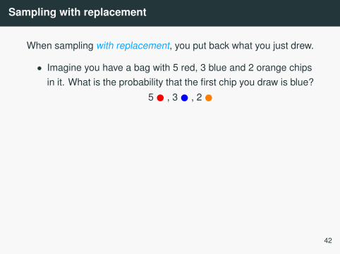
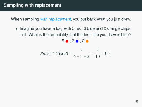
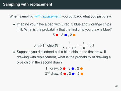
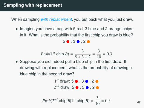
When sampling with replacement, you put back what you just drew.
• Imagine you have a bag with 5 red, 3 blue and 2 orange chipsin it. What is the probability that the first chip you draw is blue?
5 , 3 , 2
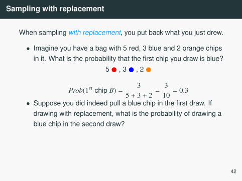
Prob(1st chip B) =3
5 + 3 + 2=
310= 0.3
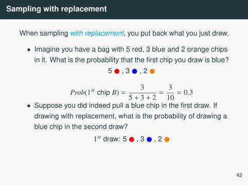
• Suppose you did indeed pull a blue chip in the first draw. Ifdrawing with replacement, what is the probability of drawing ablue chip in the second draw?
1st draw: 5 , 3 , 2 2nd draw: 5 , 3 , 2
Prob(2nd chip B|1st chip B) =3
10= 0.3
42
Sampling with replacement
When sampling with replacement, you put back what you just drew.
• Imagine you have a bag with 5 red, 3 blue and 2 orange chipsin it. What is the probability that the first chip you draw is blue?
5 , 3 , 2
Prob(1st chip B) =3
5 + 3 + 2=
310= 0.3
• Suppose you did indeed pull a blue chip in the first draw. Ifdrawing with replacement, what is the probability of drawing ablue chip in the second draw?
1st draw: 5 , 3 , 2
2nd draw: 5 , 3 , 2
Prob(2nd chip B|1st chip B) =3
10= 0.3
42
Sampling with replacement
When sampling with replacement, you put back what you just drew.
• Imagine you have a bag with 5 red, 3 blue and 2 orange chipsin it. What is the probability that the first chip you draw is blue?
5 , 3 , 2
Prob(1st chip B) =3
5 + 3 + 2=
310= 0.3
• Suppose you did indeed pull a blue chip in the first draw. Ifdrawing with replacement, what is the probability of drawing ablue chip in the second draw?
1st draw: 5 , 3 , 2 2nd draw: 5 , 3 , 2
Prob(2nd chip B|1st chip B) =3
10= 0.3
42
Sampling with replacement
When sampling with replacement, you put back what you just drew.
• Imagine you have a bag with 5 red, 3 blue and 2 orange chipsin it. What is the probability that the first chip you draw is blue?
5 , 3 , 2
Prob(1st chip B) =3
5 + 3 + 2=
310= 0.3
• Suppose you did indeed pull a blue chip in the first draw. Ifdrawing with replacement, what is the probability of drawing ablue chip in the second draw?
1st draw: 5 , 3 , 2 2nd draw: 5 , 3 , 2
Prob(2nd chip B|1st chip B) =3
10= 0.3 42
Sampling with replacement (cont.)
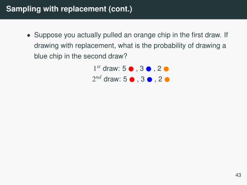
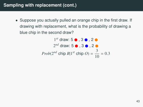
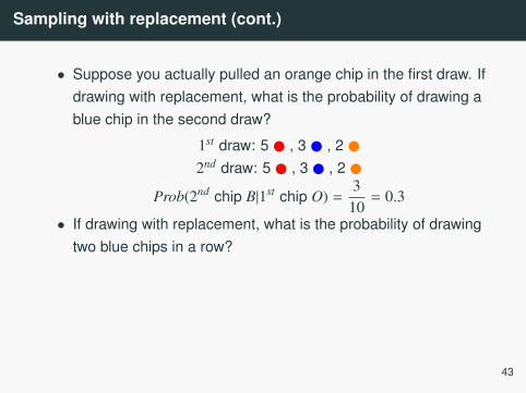
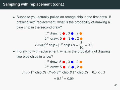
• Suppose you actually pulled an orange chip in the first draw. Ifdrawing with replacement, what is the probability of drawing ablue chip in the second draw?
1st draw: 5 , 3 , 2 2nd draw: 5 , 3 , 2
Prob(2nd chip B|1st chip O) =310= 0.3
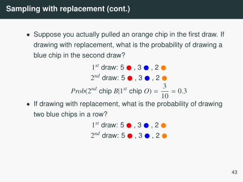
• If drawing with replacement, what is the probability of drawingtwo blue chips in a row?
1st draw: 5 , 3 , 2 2nd draw: 5 , 3 , 2
Prob(1st chip B) · Prob(2nd chip B|1st chip B) = 0.3 × 0.3
= 0.32 = 0.09
43
Sampling with replacement (cont.)
• Suppose you actually pulled an orange chip in the first draw. Ifdrawing with replacement, what is the probability of drawing ablue chip in the second draw?
1st draw: 5 , 3 , 2
2nd draw: 5 , 3 , 2
Prob(2nd chip B|1st chip O) =310= 0.3
• If drawing with replacement, what is the probability of drawingtwo blue chips in a row?
1st draw: 5 , 3 , 2 2nd draw: 5 , 3 , 2
Prob(1st chip B) · Prob(2nd chip B|1st chip B) = 0.3 × 0.3
= 0.32 = 0.09
43
Sampling with replacement (cont.)
• Suppose you actually pulled an orange chip in the first draw. Ifdrawing with replacement, what is the probability of drawing ablue chip in the second draw?
1st draw: 5 , 3 , 2 2nd draw: 5 , 3 , 2
Prob(2nd chip B|1st chip O) =310= 0.3
• If drawing with replacement, what is the probability of drawingtwo blue chips in a row?
1st draw: 5 , 3 , 2 2nd draw: 5 , 3 , 2
Prob(1st chip B) · Prob(2nd chip B|1st chip B) = 0.3 × 0.3
= 0.32 = 0.09
43
Sampling with replacement (cont.)
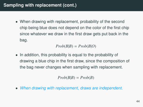
• When drawing with replacement, probability of the secondchip being blue does not depend on the color of the first chipsince whatever we draw in the first draw gets put back in thebag.
Prob(B|B) = Prob(B|O)
• In addition, this probability is equal to the probability ofdrawing a blue chip in the first draw, since the composition ofthe bag never changes when sampling with replacement.
Prob(B|B) = Prob(B)
• When drawing with replacement, draws are independent.
44
Sampling without replacement
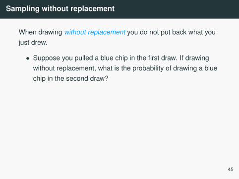
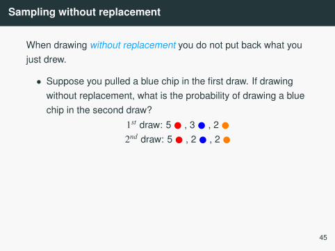
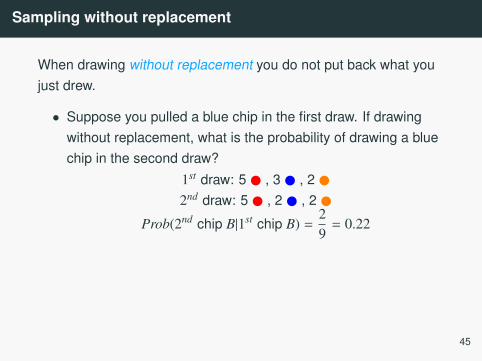
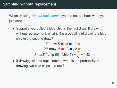
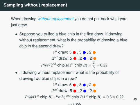
When drawing without replacement you do not put back what youjust drew.
• Suppose you pulled a blue chip in the first draw. If drawingwithout replacement, what is the probability of drawing a bluechip in the second draw?
1st draw: 5 , 3 , 2 2nd draw: 5 , 2 , 2
Prob(2nd chip B|1st chip B) =29= 0.22
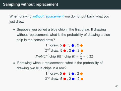
• If drawing without replacement, what is the probability ofdrawing two blue chips in a row?
1st draw: 5 , 3 , 2 2nd draw: 5 , 2 , 2
Prob(1st chip B) · Prob(2nd chip B|1st chip B) = 0.3 × 0.22
= 0.066
45
Sampling without replacement
When drawing without replacement you do not put back what youjust drew.
• Suppose you pulled a blue chip in the first draw. If drawingwithout replacement, what is the probability of drawing a bluechip in the second draw?
1st draw: 5 , 3 , 2 2nd draw: 5 , 2 , 2
Prob(2nd chip B|1st chip B) =29= 0.22
• If drawing without replacement, what is the probability ofdrawing two blue chips in a row?
1st draw: 5 , 3 , 2 2nd draw: 5 , 2 , 2
Prob(1st chip B) · Prob(2nd chip B|1st chip B) = 0.3 × 0.22
= 0.066
45

Sampling without replacement
When drawing without replacement you do not put back what youjust drew.
• Suppose you pulled a blue chip in the first draw. If drawingwithout replacement, what is the probability of drawing a bluechip in the second draw?
1st draw: 5 , 3 , 2
2nd draw: 5 , 2 , 2
Prob(2nd chip B|1st chip B) =29= 0.22
• If drawing without replacement, what is the probability ofdrawing two blue chips in a row?
1st draw: 5 , 3 , 2 2nd draw: 5 , 2 , 2
Prob(1st chip B) · Prob(2nd chip B|1st chip B) = 0.3 × 0.22
= 0.066
45
Sampling without replacement
When drawing without replacement you do not put back what youjust drew.
• Suppose you pulled a blue chip in the first draw. If drawingwithout replacement, what is the probability of drawing a bluechip in the second draw?
1st draw: 5 , 3 , 2 2nd draw: 5 , 2 , 2
Prob(2nd chip B|1st chip B) =29= 0.22
• If drawing without replacement, what is the probability ofdrawing two blue chips in a row?
1st draw: 5 , 3 , 2 2nd draw: 5 , 2 , 2
Prob(1st chip B) · Prob(2nd chip B|1st chip B) = 0.3 × 0.22
= 0.06645
Sampling without replacement (cont.)
• When drawing without replacement, the probability of thesecond chip being blue given the first was blue is not equal tothe probability of drawing a blue chip in the first draw since thecomposition of the bag changes with the outcome of the firstdraw.
Prob(B|B) , Prob(B)
• When drawing without replacement, draws are notindependent.
• This is especially important to take note of when the samplesizes are small. If we were dealing with, say, 10,000 chips in a(giant) bag, taking out one chip of any color would not have asbig an impact on the probabilities in the second draw.
46
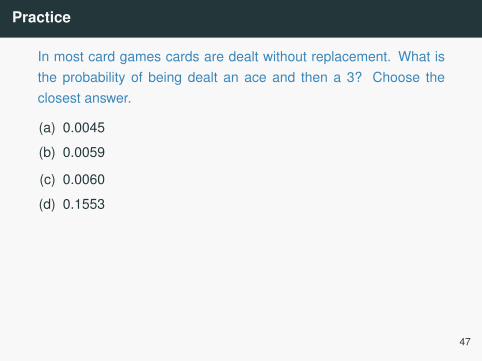
Practice
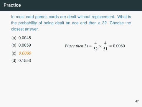
In most card games cards are dealt without replacement. What isthe probability of being dealt an ace and then a 3? Choose theclosest answer.
(a) 0.0045
(b) 0.0059
(c) 0.0060
(d) 0.1553
P(ace then 3) =4
52×
451≈ 0.0060
47
Practice
In most card games cards are dealt without replacement. What isthe probability of being dealt an ace and then a 3? Choose theclosest answer.
(a) 0.0045
(b) 0.0059
(c) 0.0060
(d) 0.1553
P(ace then 3) =4
52×
451≈ 0.0060
47
Random variables
Random variables
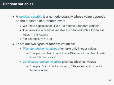
• A random variable is a numeric quantity whose value dependson the outcome of a random event• We use a capital letter, like X, to denote a random variable• The values of a random variable are denoted with a lowercase
letter, in this case x• For example, P(X = x)
• There are two types of random variables:• Discrete random variables often take only integer values
• Example: Number of credit hours, Difference in number of credithours this term vs last
• Continuous random variables take real (decimal) values• Example: Cost of books this term, Difference in cost of books
this term vs last
49
Expectation
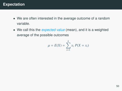
• We are often interested in the average outcome of a randomvariable.
• We call this the expected value (mean), and it is a weightedaverage of the possible outcomes
µ = E(X) =k∑
i=1
xi P(X = xi)
50
Expected value of a discrete random variable
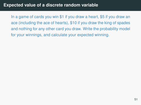
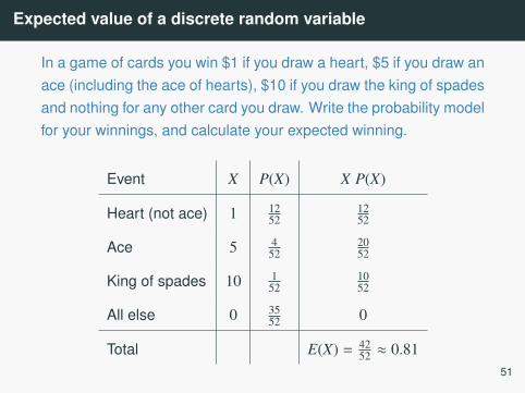
In a game of cards you win $1 if you draw a heart, $5 if you draw anace (including the ace of hearts), $10 if you draw the king of spadesand nothing for any other card you draw. Write the probability modelfor your winnings, and calculate your expected winning.
Event X P(X) X P(X)
Heart (not ace) 1 1252
1252
Ace 5 452
2052
King of spades 10 152
1052
All else 0 3552 0
Total E(X) = 4252 ≈ 0.81
51
Expected value of a discrete random variable
In a game of cards you win $1 if you draw a heart, $5 if you draw anace (including the ace of hearts), $10 if you draw the king of spadesand nothing for any other card you draw. Write the probability modelfor your winnings, and calculate your expected winning.
Event X P(X) X P(X)
Heart (not ace) 1 1252
1252
Ace 5 452
2052
King of spades 10 152
1052
All else 0 3552 0
Total E(X) = 4252 ≈ 0.81
51
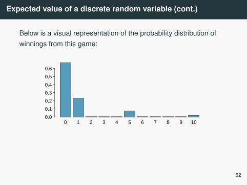
Expected value of a discrete random variable (cont.)
Below is a visual representation of the probability distribution ofwinnings from this game:
0 1 2 3 4 5 6 7 8 9 100.0
0.1
0.2
0.3
0.4
0.5
0.6
52
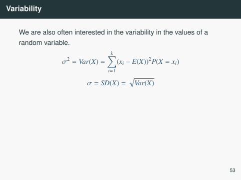
Variability
We are also often interested in the variability in the values of arandom variable.
σ2 = Var(X) =k∑
i=1
(xi − E(X))2P(X = xi)
σ = SD(X) =√
Var(X)
53
Variability of a discrete random variable
For the previous card game example, how much would you expectthe winnings to vary from game to game?
54
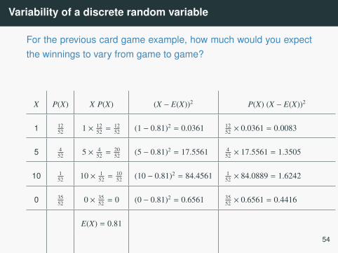
Variability of a discrete random variable
For the previous card game example, how much would you expectthe winnings to vary from game to game?
X P(X) X P(X) (X − E(X))2 P(X) (X − E(X))2
1 1252 1 × 12
52 =1252 (1 − 0.81)2 = 0.0361 12
52 × 0.0361 = 0.0083
5 452 5 × 4
52 =2052 (5 − 0.81)2 = 17.5561 4
52 × 17.5561 = 1.3505
10 152 10 × 1
52 =1052 (10 − 0.81)2 = 84.4561 1
52 × 84.0889 = 1.6242
0 3552 0 × 35
52 = 0 (0 − 0.81)2 = 0.6561 3552 × 0.6561 = 0.4416
E(X) = 0.81
54
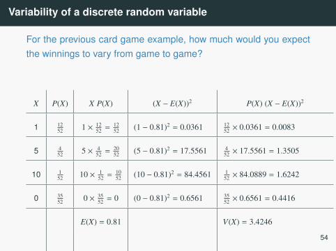
Variability of a discrete random variable
For the previous card game example, how much would you expectthe winnings to vary from game to game?
X P(X) X P(X) (X − E(X))2 P(X) (X − E(X))2
1 1252 1 × 12
52 =1252 (1 − 0.81)2 = 0.0361 12
52 × 0.0361 = 0.0083
5 452 5 × 4
52 =2052 (5 − 0.81)2 = 17.5561 4
52 × 17.5561 = 1.3505
10 152 10 × 1
52 =1052 (10 − 0.81)2 = 84.4561 1
52 × 84.0889 = 1.6242
0 3552 0 × 35
52 = 0 (0 − 0.81)2 = 0.6561 3552 × 0.6561 = 0.4416
E(X) = 0.81 V(X) = 3.4246
54
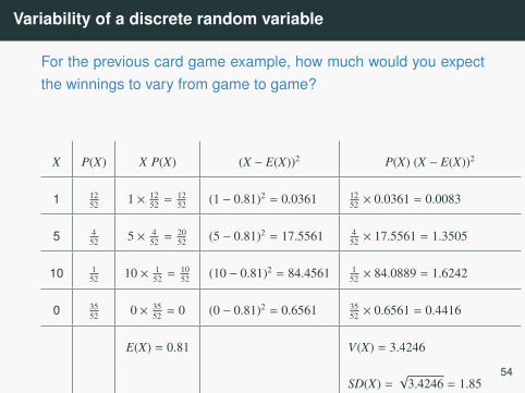
Variability of a discrete random variable
For the previous card game example, how much would you expectthe winnings to vary from game to game?
X P(X) X P(X) (X − E(X))2 P(X) (X − E(X))2
1 1252 1 × 12
52 =1252 (1 − 0.81)2 = 0.0361 12
52 × 0.0361 = 0.0083
5 452 5 × 4
52 =2052 (5 − 0.81)2 = 17.5561 4
52 × 17.5561 = 1.3505
10 152 10 × 1
52 =1052 (10 − 0.81)2 = 84.4561 1
52 × 84.0889 = 1.6242
0 3552 0 × 35
52 = 0 (0 − 0.81)2 = 0.6561 3552 × 0.6561 = 0.4416
E(X) = 0.81 V(X) = 3.4246
SD(X) =√
3.4246 = 1.8554
Linear combinations
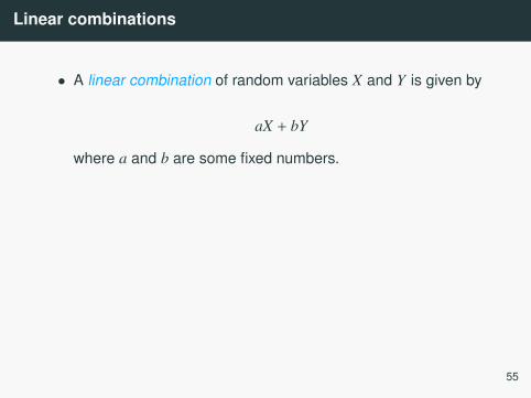
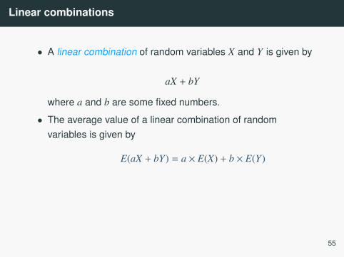
• A linear combination of random variables X and Y is given by
aX + bY
where a and b are some fixed numbers.
• The average value of a linear combination of randomvariables is given by
E(aX + bY) = a × E(X) + b × E(Y)
55
Linear combinations
• A linear combination of random variables X and Y is given by
aX + bY
where a and b are some fixed numbers.
• The average value of a linear combination of randomvariables is given by
E(aX + bY) = a × E(X) + b × E(Y)
55
Calculating the expectation of a linear combination
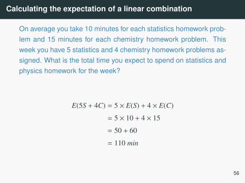
On average you take 10 minutes for each statistics homework prob-lem and 15 minutes for each chemistry homework problem. Thisweek you have 5 statistics and 4 chemistry homework problems as-signed. What is the total time you expect to spend on statistics andphysics homework for the week?
E(5S + 4C) = 5 × E(S) + 4 × E(C)
= 5 × 10 + 4 × 15
= 50 + 60
= 110 min
56
Calculating the expectation of a linear combination
On average you take 10 minutes for each statistics homework prob-lem and 15 minutes for each chemistry homework problem. Thisweek you have 5 statistics and 4 chemistry homework problems as-signed. What is the total time you expect to spend on statistics andphysics homework for the week?
E(5S + 4C) = 5 × E(S) + 4 × E(C)
= 5 × 10 + 4 × 15
= 50 + 60
= 110 min
56
Linear combinations
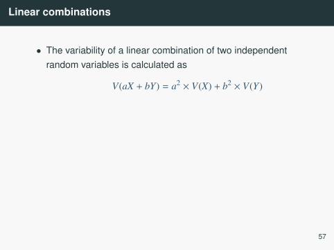
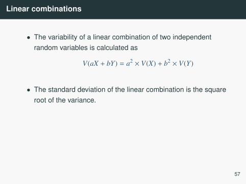
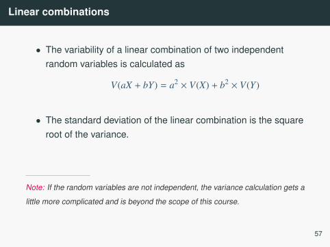
• The variability of a linear combination of two independentrandom variables is calculated as
V(aX + bY) = a2 × V(X) + b2 × V(Y)
• The standard deviation of the linear combination is the squareroot of the variance.
Note: If the random variables are not independent, the variance calculation gets a
little more complicated and is beyond the scope of this course.
57
Linear combinations
• The variability of a linear combination of two independentrandom variables is calculated as
V(aX + bY) = a2 × V(X) + b2 × V(Y)
• The standard deviation of the linear combination is the squareroot of the variance.
Note: If the random variables are not independent, the variance calculation gets a
little more complicated and is beyond the scope of this course.
57
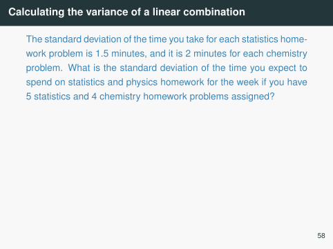
Calculating the variance of a linear combination
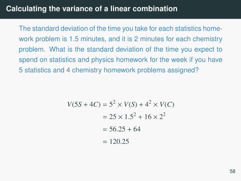
The standard deviation of the time you take for each statistics home-work problem is 1.5 minutes, and it is 2 minutes for each chemistryproblem. What is the standard deviation of the time you expect tospend on statistics and physics homework for the week if you have5 statistics and 4 chemistry homework problems assigned?
V(5S + 4C) = 52 × V(S) + 42 × V(C)
= 25 × 1.52 + 16 × 22
= 56.25 + 64
= 120.25
58
Calculating the variance of a linear combination
The standard deviation of the time you take for each statistics home-work problem is 1.5 minutes, and it is 2 minutes for each chemistryproblem. What is the standard deviation of the time you expect tospend on statistics and physics homework for the week if you have5 statistics and 4 chemistry homework problems assigned?
V(5S + 4C) = 52 × V(S) + 42 × V(C)
= 25 × 1.52 + 16 × 22
= 56.25 + 64
= 120.25
58
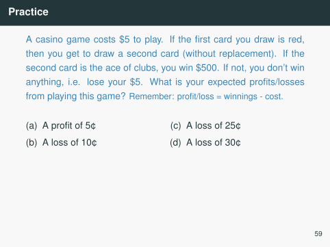
Practice
A casino game costs $5 to play. If the first card you draw is red,then you get to draw a second card (without replacement). If thesecond card is the ace of clubs, you win $500. If not, you don’t winanything, i.e. lose your $5. What is your expected profits/lossesfrom playing this game? Remember: profit/loss = winnings - cost.
(a) A profit of 5¢
(b) A loss of 10¢
(c) A loss of 25¢
(d) A loss of 30¢
59
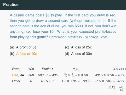
Practice
A casino game costs $5 to play. If the first card you draw is red,then you get to draw a second card (without replacement). If thesecond card is the ace of clubs, you win $500. If not, you don’t winanything, i.e. lose your $5. What is your expected profits/lossesfrom playing this game? Remember: profit/loss = winnings - cost.
(a) A profit of 5¢
(b) A loss of 10¢
(c) A loss of 25¢
(d) A loss of 30¢
Event Win Profit: X P(X) X × P(X)
Red, A♣ 500 500 - 5 = 495 2652 ×
151 = 0.0098 495 × 0.0098 = 4.851
Other 0 0 - 5 = -5 1 − 0.0098 = 0.9902 −5 × 0.9902 = −4.951
E(X) = −0.159
Fair game
A fair game is defined as a game that costs as much as itsexpected payout, i.e. expected profit is 0.
Do you think casino games in Vegas cost more or less than theirexpected payouts?
If those games cost less than theirexpected payouts, it would mean thatthe casinos would be losing money onaverage, and hence they wouldn’t beable to pay for all this:
Image by Moyan Brenn on Flickr http:// www.flickr.com/ photos/ aigle dore/ 5951714693.
60
Simplifying random variables
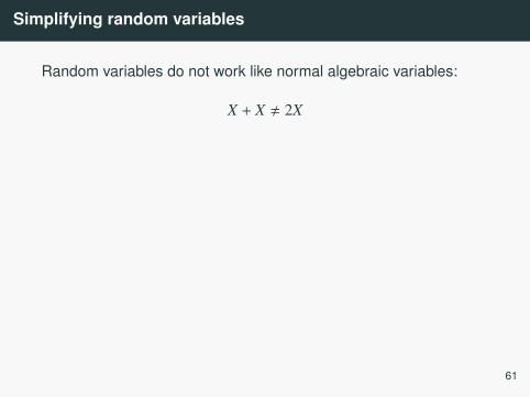
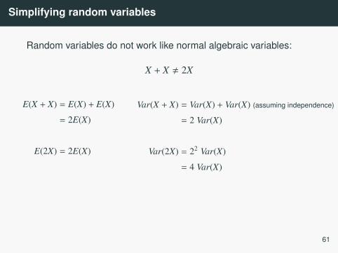
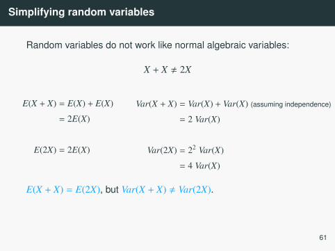
Random variables do not work like normal algebraic variables:
X + X , 2X
E(X + X) = E(X) + E(X)
= 2E(X)
E(2X) = 2E(X)
Var(X + X) = Var(X) + Var(X) (assuming independence)
= 2 Var(X)
Var(2X) = 22 Var(X)
= 4 Var(X)
E(X + X) = E(2X), but Var(X + X) , Var(2X).
61
Simplifying random variables
Random variables do not work like normal algebraic variables:
X + X , 2X
E(X + X) = E(X) + E(X)
= 2E(X)
E(2X) = 2E(X)
Var(X + X) = Var(X) + Var(X) (assuming independence)
= 2 Var(X)
Var(2X) = 22 Var(X)
= 4 Var(X)
E(X + X) = E(2X), but Var(X + X) , Var(2X).
61
Simplifying random variables
Random variables do not work like normal algebraic variables:
X + X , 2X
E(X + X) = E(X) + E(X)
= 2E(X)
E(2X) = 2E(X)
Var(X + X) = Var(X) + Var(X) (assuming independence)
= 2 Var(X)
Var(2X) = 22 Var(X)
= 4 Var(X)
E(X + X) = E(2X), but Var(X + X) , Var(2X).
61
Adding or multiplying?
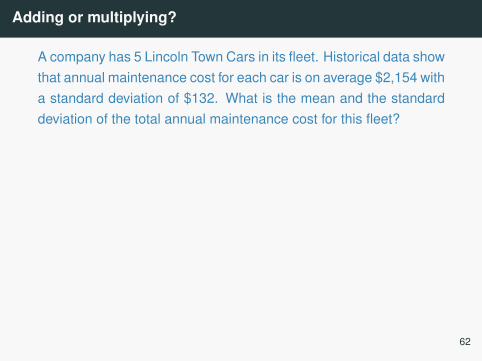
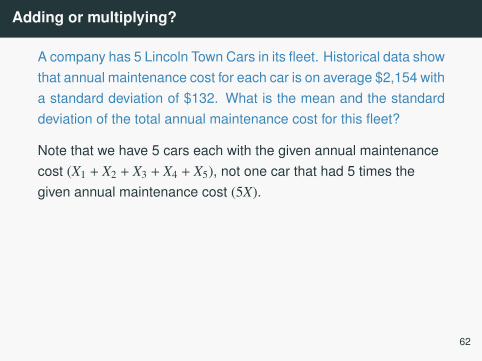
A company has 5 Lincoln Town Cars in its fleet. Historical data showthat annual maintenance cost for each car is on average $2,154 witha standard deviation of $132. What is the mean and the standarddeviation of the total annual maintenance cost for this fleet?
Note that we have 5 cars each with the given annual maintenancecost (X1 + X2 + X3 + X4 + X5), not one car that had 5 times thegiven annual maintenance cost (5X).
E(X1 + X2 + X3 + X4 + X5) = E(X1) + E(X2) + E(X3) + E(X4) + E(X5)
= 5 × E(X) = 5 × 2, 154 = $10, 770
Var(X1 + X2 + X3 + X4 + X5) = Var(X1) + Var(X2) + Var(X3) + Var(X4) + Var(X5)
= 5 × V(X) = 5 × 1322 = $87, 120
SD(X1 + X2 + X3 + X4 + X5) =√
87, 120 = 295.16
62
Adding or multiplying?
A company has 5 Lincoln Town Cars in its fleet. Historical data showthat annual maintenance cost for each car is on average $2,154 witha standard deviation of $132. What is the mean and the standarddeviation of the total annual maintenance cost for this fleet?
Note that we have 5 cars each with the given annual maintenancecost (X1 + X2 + X3 + X4 + X5), not one car that had 5 times thegiven annual maintenance cost (5X).
E(X1 + X2 + X3 + X4 + X5) = E(X1) + E(X2) + E(X3) + E(X4) + E(X5)
= 5 × E(X) = 5 × 2, 154 = $10, 770
Var(X1 + X2 + X3 + X4 + X5) = Var(X1) + Var(X2) + Var(X3) + Var(X4) + Var(X5)
= 5 × V(X) = 5 × 1322 = $87, 120
SD(X1 + X2 + X3 + X4 + X5) =√
87, 120 = 295.16
62
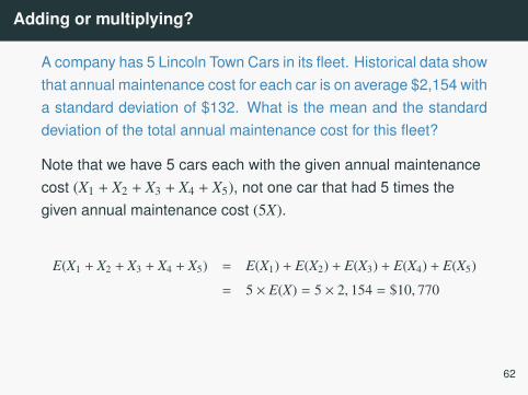
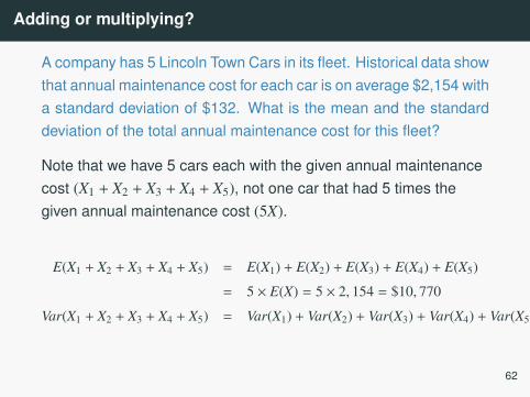
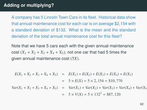
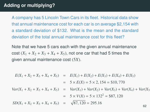
Adding or multiplying?
A company has 5 Lincoln Town Cars in its fleet. Historical data showthat annual maintenance cost for each car is on average $2,154 witha standard deviation of $132. What is the mean and the standarddeviation of the total annual maintenance cost for this fleet?
Note that we have 5 cars each with the given annual maintenancecost (X1 + X2 + X3 + X4 + X5), not one car that had 5 times thegiven annual maintenance cost (5X).
E(X1 + X2 + X3 + X4 + X5) = E(X1) + E(X2) + E(X3) + E(X4) + E(X5)
= 5 × E(X) = 5 × 2, 154 = $10, 770
Var(X1 + X2 + X3 + X4 + X5) = Var(X1) + Var(X2) + Var(X3) + Var(X4) + Var(X5)
= 5 × V(X) = 5 × 1322 = $87, 120
SD(X1 + X2 + X3 + X4 + X5) =√
87, 120 = 295.1662
Continuous distributions
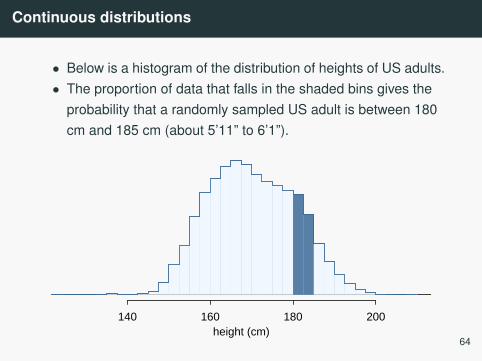
Continuous distributions
• Below is a histogram of the distribution of heights of US adults.• The proportion of data that falls in the shaded bins gives the
probability that a randomly sampled US adult is between 180cm and 185 cm (about 5’11” to 6’1”).
height (cm)140 160 180 200
64
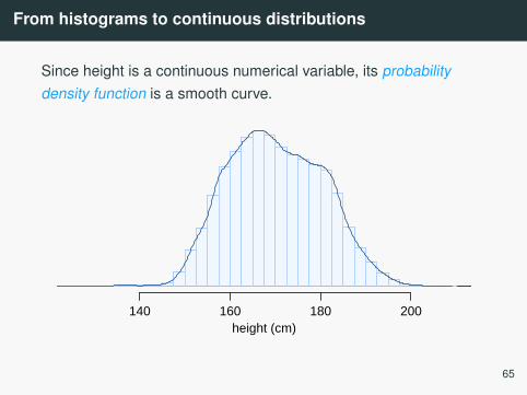
From histograms to continuous distributions
Since height is a continuous numerical variable, its probabilitydensity function is a smooth curve.
height (cm)140 160 180 200
65

Probabilities from continuous distributions
Therefore, the probability that a randomly sampled US adult isbetween 180 cm and 185 cm can also be estimated as the shadedarea under the curve.
height (cm)140 160 180 200
66
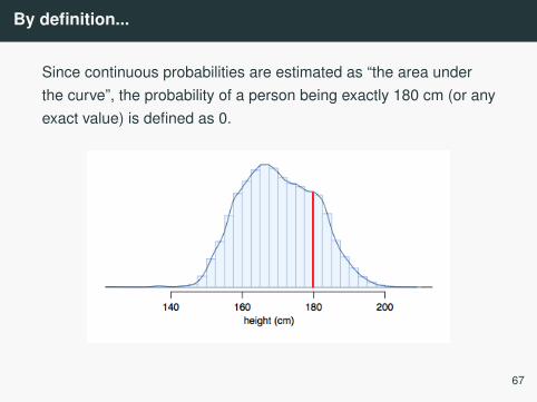
By definition...
Since continuous probabilities are estimated as “the area underthe curve”, the probability of a person being exactly 180 cm (or anyexact value) is defined as 0.
67


![Sequential Determinantal Point Processes (SeqDPPs) and ...boqinggong.info/assets/dpp.pdfSequential DPP (seqDPP) Conditional probability: still a DPP ! [NIPS’14] Advantages of SeqDPP](https://img.pdfslide.us/doc/110x75/613a85000051793c8c0116a7/sequential-determinantal-point-processes-seqdpps-and-sequential-dpp-seqdpp.jpg)