Chapter 2: Preliminaries and elements of convex analysishome.deib.polimi.it/.../preliminaries-convex-analysis-14-15.pdf · Chapter 2: Preliminaries and elements of convex analysis

Chapter 2: Preliminaries and elements of convex

analysis

Edoardo Amaldi

DEIB – Politecnico di [email protected]

Website: http://home.deib.polimi.it/amaldi/OPT-14-15.shtml

Academic year 2014-15

Edoardo Amaldi (PoliMI) Optimization Academic year 2014-15 1 / 23

http://home.deib.polimi.it/amaldi/OPT-14-15.shtml

2.1 Basic concepts

In Rn with Euclidean norm

x ∈ S ⊆ Rn is an interior point of S if ∃ ε > 0 such that

Bε(x) = {y ∈ Rn : ‖y − x‖ < ε} ⊆ S .

x ∈ Rn is a boundary point of S if, for every ε > 0, Bε(x) contains at least one

point of S and one point of its complement Rn \ S .

The set of all the interior points of S ⊆ Rn is the interior of S , denoted by int(S).

The set of all boundary points of S is the boundary of S , denoted by ∂(S).

S ⊆ Rn is open if S = int(S); S is closed if its complement is open. Intuitively, a

closed set contains all the points in ∂(S).

S ⊆ Rn is bounded if ∃ M > 0 such that ‖x‖ ≤ M for every x ∈ S .

S ⊆ Rn closed and bounded is compact.


Property:

A set S ⊆ Rn is closed if and only if every sequence {x i}i∈N ⊆ S that converges,

converges to x ∈ S .

A set S ⊆ Rn is compact if and only if every sequence {x i}i∈N ⊆ S admits a subsequence

that converges to a point x ∈ S .


Existence of an optimal solution

In general, when we wish to minimize a function f : S ⊆ Rn → R, we only know that

there exists a greatest lower bound (infimum), that is

infx∈S

f (x)

Theorem (Weierstrass):

Let S ⊆ Rn be nonempty and compact set, and f : S → R be continuous on S . Then

there exists a x∗ ∈ S such that f (x∗) ≤ f (x) for every x ∈ S .

Examples in which the result does not hold because: S is not closed, S is not bounded orf (x) is not continuous on S .

Since the problem admits an optimal solution x∗ ∈ S , we can write minx∈S f (x).

Observation: this result holds in any vector space of finite dimension.


Cones and affine subspaces

Consider any subset S ⊂ Rn

Definition: cone(S) denotes the set of all the conic combinations of points of S , i.e., allthe points x ∈ R

n such that x =∑m

i=1 αi x i with x1, . . . , xm ∈ S and αi ≥ 0 per every i ,1 ≤ i ≤ m.

Examples: polyedral cone generated by a finite number of vectors, ”ice cream” cone in

R3 generated by an infinite number of vectors

Definition: aff(S) denotes the smallest affine subspace that contains S .

aff(S) coincides with the set of all the affine combinations of points in S , i.e., all thepoints x ∈ R

n such that x =∑m

i=1 αi x i with x1, . . . , xm ∈ S and with∑m

i=1 αi = 1,where αi ∈ R for every i , 1 ≤ i ≤ m.

Examples: straight line containing two points in R2, plane containing three points in

general position in R3


2.2 Elements of convex analysis

Definition:

A set C ⊂ Rn is convex if

αx1 + (1− α)x2 ∈ C ∀x1, x2 ∈ C and ∀α ∈ [0, 1].

A point x ∈ Rn is a convex combination of x1, . . . , xm ∈ R

n se

x =m∑

i=1

αi x i

with αi ≥ 0 for every i , 1 ≤ i ≤ m, and∑m

i=1 αi = 1.

Property: If Ci with i = 1, . . . , k are convex, then ∩ki=1Ci is convex.


Examples of convex sets

1) Hyperplane H = {x ∈ Rn : ptx = β} with p 6= 0.

For x ∈ H, ptx = β implies H = {x ∈ Rn : pt(x − x) = 0} and hence H is the set of all

the vectors in Rn orthogonal to p.

N.B.: H is closed since H = ∂(H)

2) Closed half-spaces H+ = {x ∈ Rn : ptx ≥ β} and H− = {x ∈ R

n : ptx ≤ β} withp 6= 0.

3) Feasible region X = {x ∈ Rn : Ax ≥ b, x ≥ 0} of a Linear Program (LP)

min c tx

s.t. Ax ≥ b

x ≥ 0

X is a convex and closed subset (intersection of m + n closed half-spaces if A ∈ Rm×n).


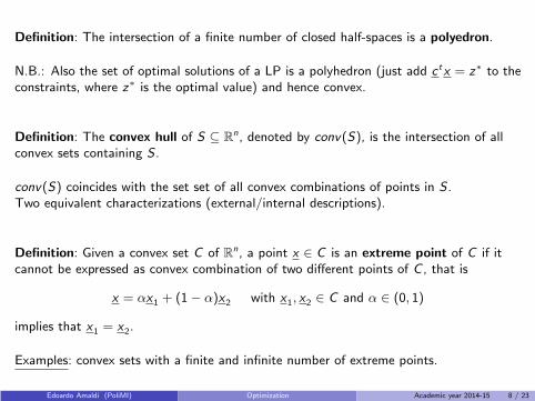
Definition: The intersection of a finite number of closed half-spaces is a polyedron.

N.B.: Also the set of optimal solutions of a LP is a polyhedron (just add c tx = z∗ to theconstraints, where z∗ is the optimal value) and hence convex.

Definition: The convex hull of S ⊆ Rn, denoted by conv(S), is the intersection of all

convex sets containing S .

conv(S) coincides with the set set of all convex combinations of points in S .Two equivalent characterizations (external/internal descriptions).

Definition: Given a convex set C of Rn, a point x ∈ C is an extreme point of C if itcannot be expressed as convex combination of two different points of C , that is

x = αx1 + (1− α)x2 with x1, x2 ∈ C and α ∈ (0, 1)

implies that x1 = x2.

Examples: convex sets with a finite and infinite number of extreme points.


Projection on a convex set

Projection of a point on a subset to which it does not belong to.

Lemma (Projection):

Let C ⊆ Rn be a nonempty, closed and convex set, then for every y 6∈ C there exists a

unique x ′ ∈ C at minimum distance from y .

Moreover, x ′ ∈ C is the closest point to y if and only if

(y − x ′)t(x − x ′) ≤ 0 ∀x ∈ C .

Definition: x ′ is the projection of y on C .

Geometric illustration:

Proof:


Separation theorem and consequences

Geometrically intuitive but fundamental result.

Theorem (Separating hyperplane)

Let C ⊂ Rn be a nonempty, closed and convex set and y 6∈ C , then there exists a p ∈ R

n

such that ptx < pty for every x ∈ C .

Thus there exists a hyperplane H = {x ∈ Rn : ptx = β} with p 6= 0 that separates y

from C , i.e., such that

C ⊆ H− = {x ∈ Rn : ptx ≤ β} and y 6∈ H− (pty > β)

Geometric illustration:

Proof: According to the Lemma, (y − x ′)t(x − x ′) ≤ 0 ∀x ∈ C .

Taking p = (y − x ′) 6= 0 and β = (y − x ′)tx ′ we have ptx ≤ β ∀x ∈ C ,

while pty − β = (y − x ′)t(y − x ′) = ‖y − x ′‖2 > 0 since y 6∈ C .


Three important consequences:

1) Any nonempty, closed and convex set C ⊆ Rn is the intersection of all closed

half-spaces containing it.

Definition: Let S ⊂ Rn be nonempty and x ∈ ∂(S) ( boundary w.r.t. aff(S) ),

H = {x ∈ Rn : pt(x − x) = 0} is a supporting hyperplane of S at x if S ⊆ H− or

S ⊆ H+.

2) Supporting hyperplane:

If C 6= ∅ is a convex set in Rn, then for every x ∈ ∂(C) there exists a supporting

hyperplane H at x , i.e., ∃ p 6= 0 such that pt(x − x) ≤ 0, for each x ∈ C .

A convex set admits at least a supporting hyperplane at each boundary point. Fornonconvex sets, such a hyperplane may not exist.

Examples: cases with 1/∞/0 supporting hyperplanes in a given boundary point x

Proof sketch:


Central result of Optimization (also of Game theory) from which we will derive theoptimality conditions for Nonlinear Programming.

3) Farkas Lemma:

Let A ∈ Rm×n and b ∈ R

m. Then

∃ x ∈ Rn such that Ax = b and x ≥ 0 ⇔ 6 ∃ y ∈ R

m such that y tA ≤ 0t e y tb > 0.

In this form, it provides an infeasibility certificate for a given linear system, but it is alsoknown as the theorem of the alternative.

Alternative: exactly one of the two systems Ax = b, x ≥ 0 and y tA ≤ 0t , y tb > 0 isfeasible.

Geometric interpretation:

b belongs to the convex cone generated by the columns A1, . . . ,An of A, i.e., tocone(A)= {z ∈ R

m : z =∑n

j=1 αj Aj , α1 ≥ 0, . . . , αn ≥ 0}, if and only if no hyperplaneseparating b from cone(A) exists.

Alternative: b ∈ cone(A) or b 6∈ cone(A) (hence ∃ hyperplane separating b from cone(A))


Proof:


Application of Farkas Lemma: asset pricing in absence of arbitrage

Single period, m assets are traded, n possible states (scenarios).

Assets can be bought or sold “short”, i.e., with the promise to buy them back at theend.

Portfolio y ∈ Rm, with yi = amount invested in asset i .

A negative value of yi indicates a ”short” position.

If pi is the price of a unit of asset i at the beginning, the portfolio cost is: pty

Consider A ∈ Rm×n with aij = value of one euro invested in asset i if state j occurs.

At the end all assets are sold (we receive a payoff of aijyi ) and the “short” positions arecovered (we pay aij |yi | and hence have a payoff of aijyi ).

Portfolio value: v t = y tA

Absence of arbitrage condition: any portfolio with nonnegative values for all states musthave a nonnegative cost.

Algebraically: 6 ∃ y such that y tA ≥ 0t and pty < 0.


According to Farkas Lemma:

No possibility of arbitrage exist ( 6 ∃ y such that y tA ≥ 0t and pty < 0 )

if and only if

∃ q ∈ Rn with q ≥ 0 such that the asset price vector p satisfies

Aq = p.

If the market is efficient, some ”state prices” qi exist.

N.B.: in general q is not unique.


2.2.2 Convex functions

Definitions:

A function f : C → R defined on a convex set C ⊆ Rn is convex if

f (αx1 + (1− α)x2) ≤ αf (x1) + (1− α)f (x2) ∀x1, x2 ∈ C and ∀α ∈ [0, 1],

f is strictly convex if the inequality holds with < for ∀x1, x2 ∈ C with x1 6= x2 and

∀α ∈ (0, 1).

f is concave if −f is convex.

The epigraph of f : S ⊆ Rn → R, denoted by epi(f ), is the subset of Rn+1

epi(f ) = {(x , y) ∈ S × R : f (x) ≤ y}.

Let f : C → R be convex, the domain of f is the subset of Rn

dom(f ) = {x ∈ C : f (x) < +∞}.


Property:

Let C ⊆ Rn be a (nonempty) convex set and f : C → R be a convex function.

For each real β (also for +∞), the level set

Lβ = {x ∈ C : f (x) ≤ β} and {x ∈ C : f (x) < β}

is a convex subset of Rn.

The function f is continuous in the relative interior (with respect to aff(C)) of itsdomain.

The function f is convex if and only if epi(f ) is a convex subset of Rn+1 (exercise1.3).


Optimal solution of convex problems

Consider minx∈C⊆Rn f (x) where C ⊆ Rn is a convex set and f is a convex function.

Proposition:

If C ⊆ Rn is convex and f : C → R is convex, each local minimum of f on C is a global

minimum.

If f is strictly convex on C , then there exists at most one global minimum (the problemcould be unbounded).

Proof: Suppose x ′ is a local minimum and ∃ x∗ ∈ C such that f (x∗) < f (x ′).

Since f is convex

f (αx ′ + (1− α)x∗) ≤ αf (x ′) + (1− α)f (x∗) < f (x ′) ∀α ∈ (0, 1)

contradicts the fact that x ′ is a local minimum.

If f is strictly convex and x∗1 and x∗

2 are two global minima, the convexity of C implies

1

2(x∗

1 + x∗2 ) ∈ C

and strict convexity of f implies

f (1

2(x∗

1 + x∗2 )) <

1

2f (x∗

1 ) +1

2f (x∗

2 ).

Thus x∗1 and x∗

2 cannot be two global minima.Edoardo Amaldi (PoliMI) Optimization Academic year 2014-15 18 / 23

Characterizations of convex functions

1) Proposition: A continuously differentiable function (of class C1) f : C → R definedon an open and nonempty convex set C ⊆ R

n is convex if and only if

f (x) ≥ f (x) +∇t f (x)(x − x) ∀x , x ∈ C .

f is strictly convex if and only if the inequality holds with > for every pair x , x ∈ C withx 6= x .

Definition: Directional derivative of f : limα→0+f (x+α(x−x))−f (x)

α= ∇t f (x)(x − x)

Geometric interpretation:

The linear approximation of f at x (1st order Taylor’s expansion) bounds below f (x) and

H = {

(

xy

)

∈ Rn+1 : (∇t f (x) − 1)

(

xy

)

= −f (x) +∇t f (x) x }

is a supporting hyperplane of epi(f ) in (x , f (x)), with epi(f ) ⊆ H−.


2) Proposition: A twice continuously differentiable function (of class C2) f : C → R

defined on an open and nonempty convex set C ⊆ Rn is convex if and only if the Hessian

matrix ∇2f (x) = ( ∂2f∂xi∂xj

) is positive semidefinite at every x ∈ S .

For C2 functions, if ∇2f (x) is positive definite ∀x ∈ C then f (x) is strictly convex.

N.B.: This condition is sufficient but not necessary: f (x) = x4 is strictly convex butf ′′(0) = 0.

Definition:A symmetric matrix A n × n is positive definite if y tAy > 0 ∀y ∈ R

n with y 6= 0,

A symmetric matrix A n × n is positive semidefinite if y tAy ≥ 0 ∀y ∈ Rn.

Equivalent definitions: based on the sign of the eigenvalues/principal minors of A or ofthe diagonal coefficients of specific factorizations of A (e.g., Cholesky factorization).


Subgradient of convex and concave functions

Convex/concave (continuous) functions that are not everywhere differentiable, e.g.f (x) = |x |.

Generalization of the concept of gradient for C1 functions to piecewise C1 functions.

Definitions: Let C ⊆ Rn be a convex set and f : C → R be a convex function on C

• a vector γ ∈ Rn is a subgradient of f at x ∈ C if

f (x) ≥ f (x) + γt(x − x) ∀x ∈ C ,

• the subdifferential, denoted by ∂f (x), is the set of all the subgradients of f at x .

Example: For f (x) = x2, in x = 3 the only subgradient is γ = 6.

Indeed, 0 ≤ (x − 3)2 = x2 − 6x + 9 implies for every x :

f (x) = x2 ≥ 6x − 9 = 9 + 6(x − 3) = f (x) + 6(x − x)


Other examples:

1) For f (x) = |x | it is clear that: γ = 1 if x > 0, γ = −1 if x < 0, ∂f (x) = [−1, 1] ifx = 0.

2) Consider f (x) = min{f1(x), f2(x)} with f1(x) = 4− |x | and f2(x) = 4− (x − 2)2.

Since f2(x) ≥ f1(x) for 1 ≤ x ≤ 4,

f (x) =

{

4− x 1 ≤ x ≤ 44− (x − 2)2 otherwise

γ = −1 for x ∈ (1, 4),

γ = −2(x − 2) for x < 1 or x > 4,

γ ∈ [−1, 2] at x = 1,

γ ∈ [−4,−1] at x = 4.


Properties:

1) A convex function f : C → R admits at least a subgradient at every interior point x ofC . In particular, if x ∈ int(C) then there exists γ ∈ R

n such that

H = {(x , y) ∈ Rn+1 : y = f (x) + γ

t(x − x)}

is a supporting hyperplane of epi(f ) at (x , f (x)).

N.B.: The existence of (at least) a subgradient at every point of int(C), with C convex,is a necessary and sufficient condition for f to be convex on int(C).

2) If f is a convex function and x ∈ C , ∂f (x) is a nonempty, convex, closed and boundedset.

3) x∗ is a (global) minimum of a convex function f : C → R if and only if 0 ∈ ∂f (x∗).


Documents

Chapter 2: Preliminaries and elements of convex analysishome.deib.polimi.it/.../preliminaries-convex-analysis-14-15.pdf · Chapter 2: Preliminaries and elements of convex analysis