Embed Size (px)
Citation preview
1
Nesterov’sOptimal Gradient Methods
Xinhua Zhang
Australian National UniversityNICTA
Yurii Nesterovhttp://www.core.ucl.ac.be/~nesterov
2
Outlinen The problem from machine learning perspectiven Preliminaries
n Convex analysis and gradient descentn Nesterov’s optimal gradient method
n Lower bound of optimizationn Optimal gradient method
n Utilizing structure: composite optimizationn Smooth minimizationn Excessive gap minimization
n Conclusion
3
Outlinen The problem from machine learning perspectiven Preliminaries
n Convex analysis and gradient descentn Nesterov’s optimal gradient method
n Lower bound of optimizationn Optimal gradient method
n Utilizing structure: composite optimizationn Smooth minimizationn Excessive gap minimization
n Conclusion
4
The problem
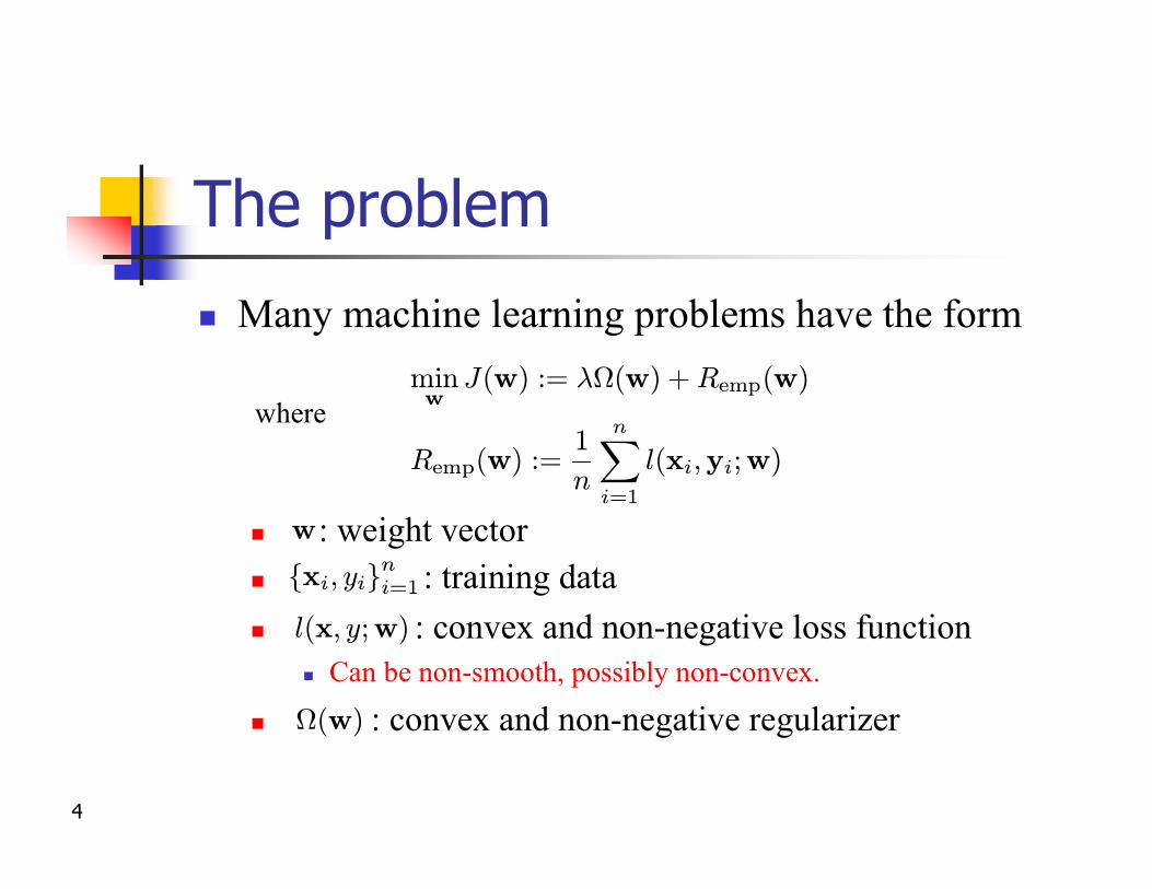
n Many machine learning problems have the form
n : weight vectorn : training datan : convex and non-negative loss function
n Can be non-smooth, possibly non-convex.
n : convex and non-negative regularizer
minw
J(w) := ¸(w) + Remp(w)
Remp(w) :=1
n
nX
i=1
l(xi;yi;w)
where
w
fxi; yigni=1
l(x; y;w)
(w)
5
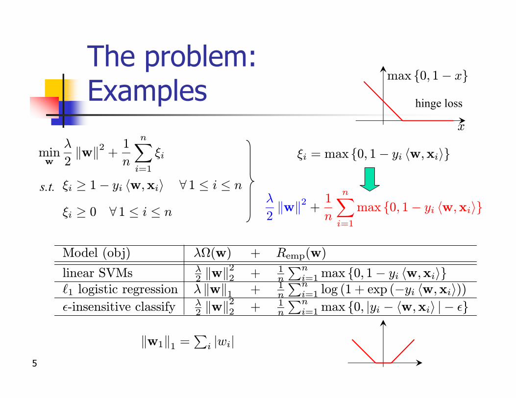
The problem:Examples
Model (obj) ¸(w) + Remp(w)
linear SVMs ¸2 kwk2
2 + 1n
Pni=1 max f0; 1¡ yi hw;xiig
`1 logistic regression ¸ kwk1 + 1n
Pni=1 log (1 + exp (¡yi hw;xii))
²-insensitive classify ¸2 kwk2
2 + 1n
Pni=1 max f0; jyi ¡ hw;xii j¡ ²g
s.t.
»i ¸ 0 8 1 · i · n
»i = max f0; 1¡ yi hw;xiig
¸
2kwk2
+1
n
nX
i=1
max f0; 1¡ yi hw;xiig
max f0; 1¡ xg
x
hinge loss
kw1k1 =P
i jwij
»i ¸ 1¡ yi hw;xii 8 1 · i · n
minw
¸
2kwk2
+1
n
nX
i=1
»i
6
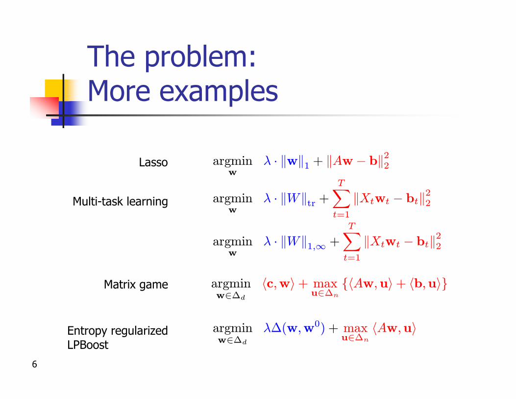
The problem:More examples
Lasso
Multi-task learning
Matrix game
Entropy regularizedLPBoost
argminw
¸ ¢ kwk1 + kAw¡ bk22
argminw
¸ ¢ kWktr +
TX
t=1
kXtwt ¡ btk22
argminw
¸ ¢ kWk1;1 +
TX
t=1
kXtwt ¡ btk22
argminw2¢d
hc;wi + maxu2¢n
fhAw;ui + hb;uig
argminw2¢d
¸¢(w;w0) + maxu2¢n
hAw;ui
7
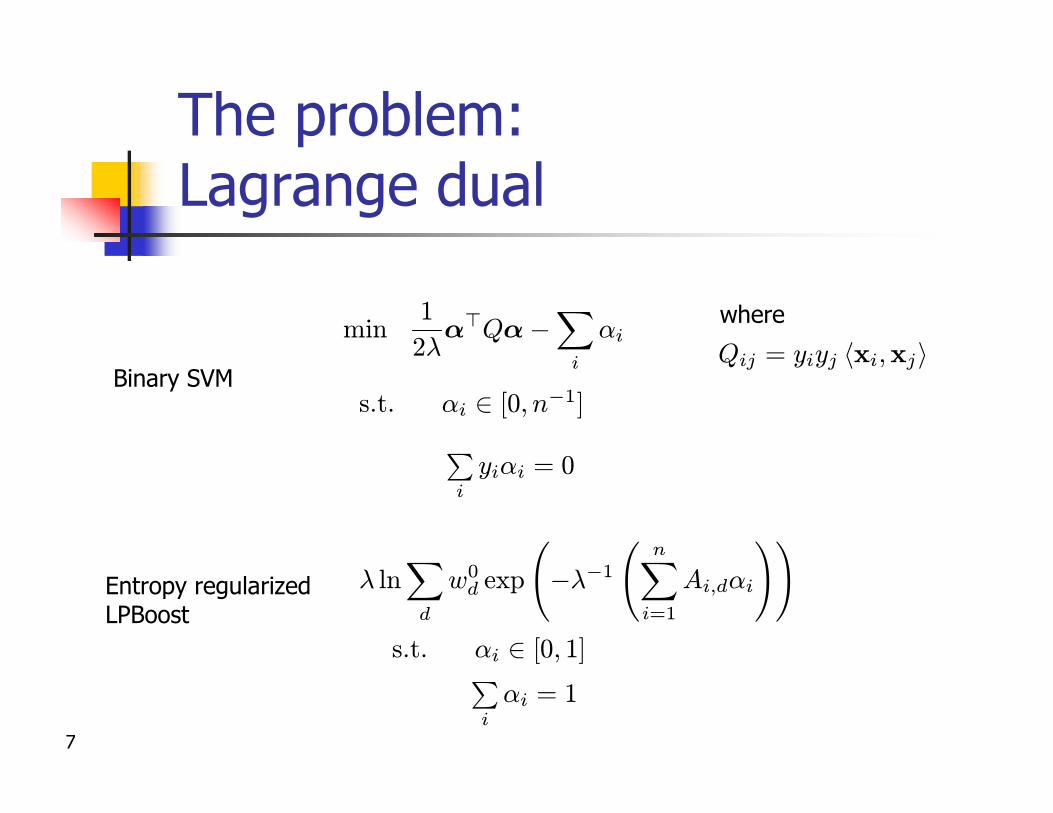
The problem:Lagrange dual
Qij = yiyj hxi;xjimin
1
2¸®>Q®¡
X
i
®i
s.t. ®i 2 [0; n¡1]
Pi
yi®i = 0
where
Binary SVM
Entropy regularizedLPBoost
s.t. ®i 2 [0; 1]Pi®i = 1
¸ lnX
d
w0d exp
ḡ1
ÃnX
i=1
Ai;d®i
!!
8
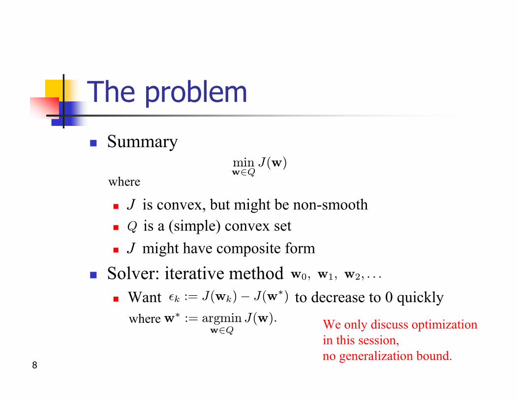
The problem
n Summary
n J is convex, but might be non-smoothn is a (simple) convex setn J might have composite form
n Solver: iterative method n Want to decrease to 0 quickly
.
whereminw2Q
J(w)
Q
w0; w1; w2; : : :
²k := J(wk)¡ J(w¤)
w¤ := argminw2Q
J(w) We only discuss optimization in this session, no generalization bound.
where
9
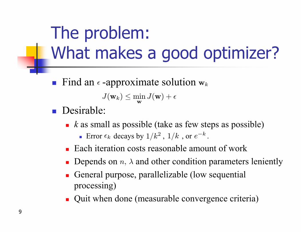
The problem:What makes a good optimizer?
n Find an -approximate solution
n Desirable:n k as small as possible (take as few steps as possible)
n Error decays by , , or .
n Each iteration costs reasonable amount of workn Depends on and other condition parameters lenientlyn General purpose, parallelizable (low sequential
processing)n Quit when done (measurable convergence criteria)
n, ¸
1=k2 1=k e¡k
wk
J(wk) · minw
J(w) + ²
²
²k
10
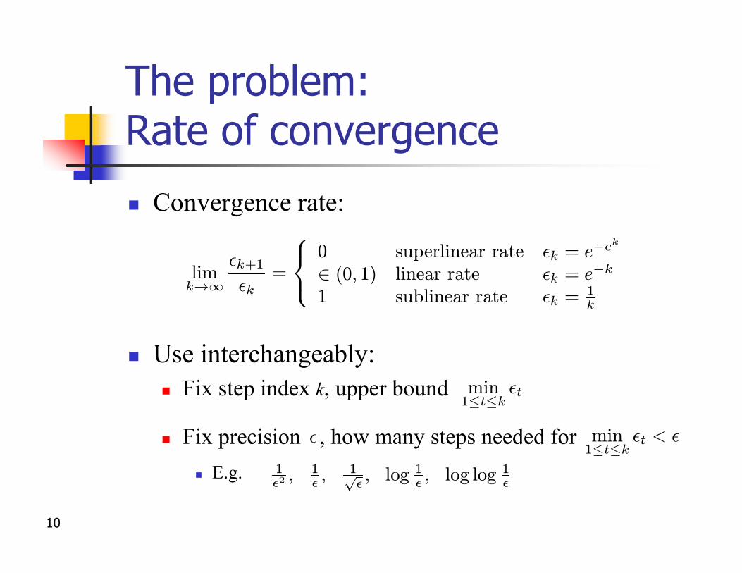
The problem:Rate of convergence
n Convergence rate:
n Use interchangeably:n Fix step index k, upper bound
n Fix precision , how many steps needed forn E.g.
min1·t·k
²t
² min1·t·k
²t < ²
1²2 ; 1
² ;1p²; log 1
² ; log log 1²
limk!1
²k+1
²k=
8<:
0 superlinear rate ²k = e¡ek
2 (0; 1) linear rate ²k = e¡k
1 sublinear rate ²k = 1k
11
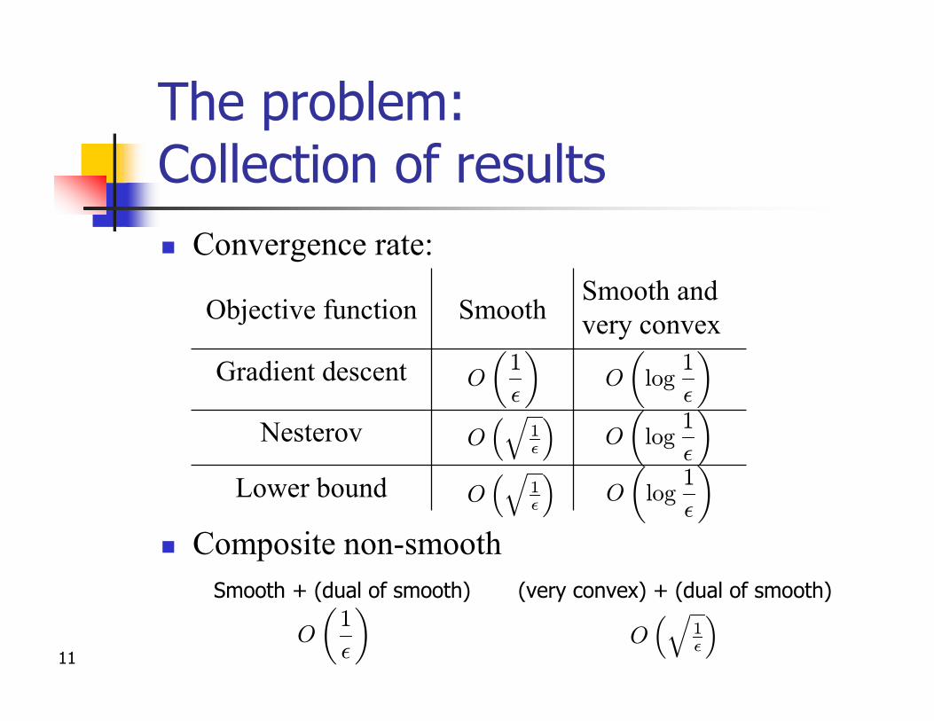
The problem:Collection of resultsn Convergence rate:
n Composite non-smooth
Lower bound
Nesterov
Gradient descent
Smooth and very convexSmoothObjective function
O
µ1
²
¶O
µlog
1
²
O
µlog
1
²
O
µlog
1
²
Smooth + (dual of smooth)
O
µ1
²
¶ (very convex) + (dual of smooth)
O³q
1²
´
O³q
1²
´
O³q
1²
´
12
Outlinen The problem from machine learning perspectiven Preliminaries
n Convex analysis and gradient descentn Nesterov’s optimal gradient method
n Lower bound of optimizationn Optimal gradient method
n Utilizing structure: composite optimizationn Smooth minimizationn Excessive gap minimization
n Conclusion
13
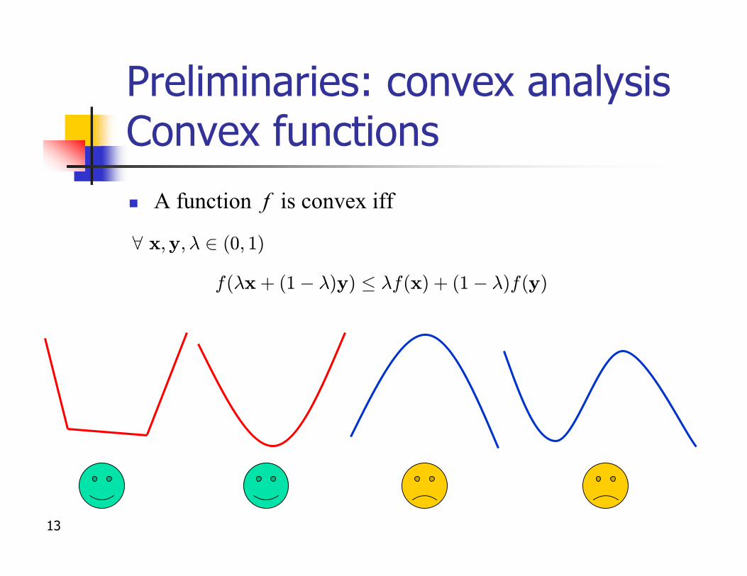
Preliminaries: convex analysisConvex functionsn A function f is convex iff
f(¸x + (1¡ ¸)y) · ¸f(x) + (1¡ ¸)f(y)
8 x;y;¸ 2 (0; 1)
14
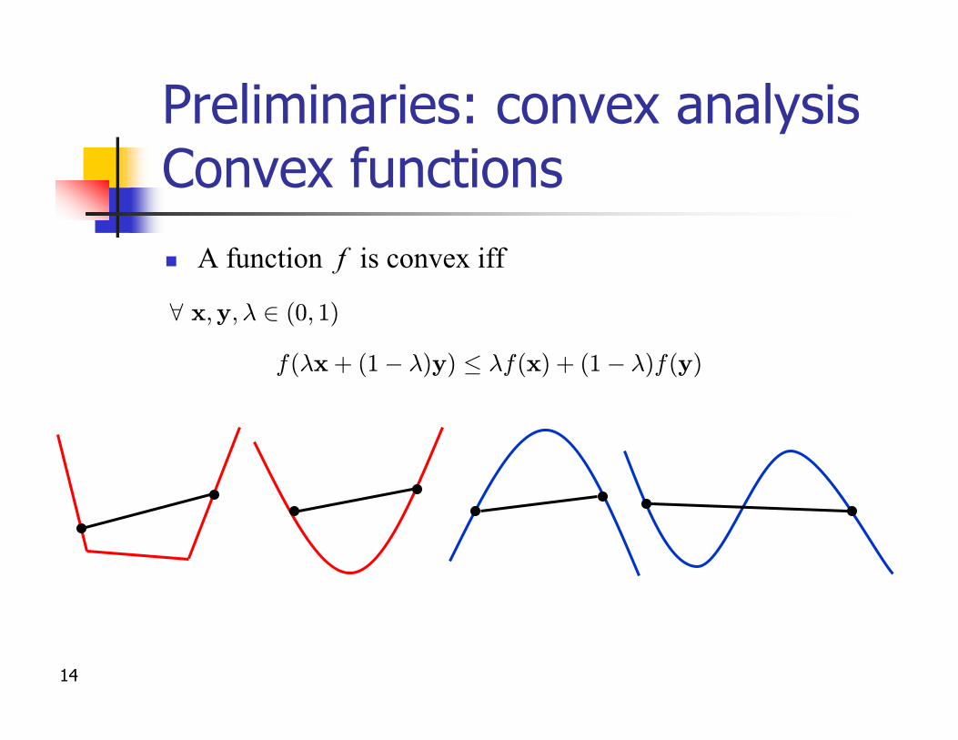
Preliminaries: convex analysisConvex functionsn A function f is convex iff
f(¸x + (1¡ ¸)y) · ¸f(x) + (1¡ ¸)f(y)
8 x;y;¸ 2 (0; 1)
15
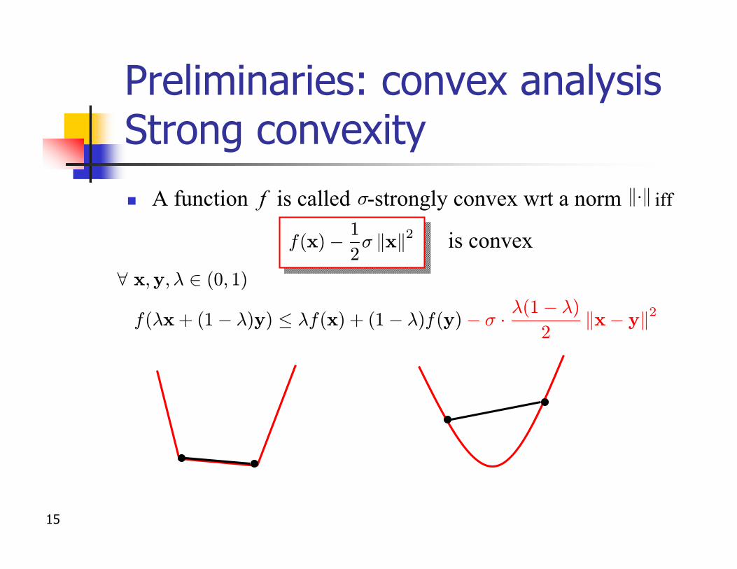
Preliminaries: convex analysisStrong convexityn A function f is called -strongly convex wrt a norm iff
f(¸x + (1¡ ¸)y) · ¸f(x) + (1¡ ¸)f(y)¡ ¾ ¢ ¸(1¡ ¸)
2kx¡ yk2
¾ k¢k
8 x;y;¸ 2 (0; 1)
f(x)¡ 1
2¾ kxk2 is convex
16
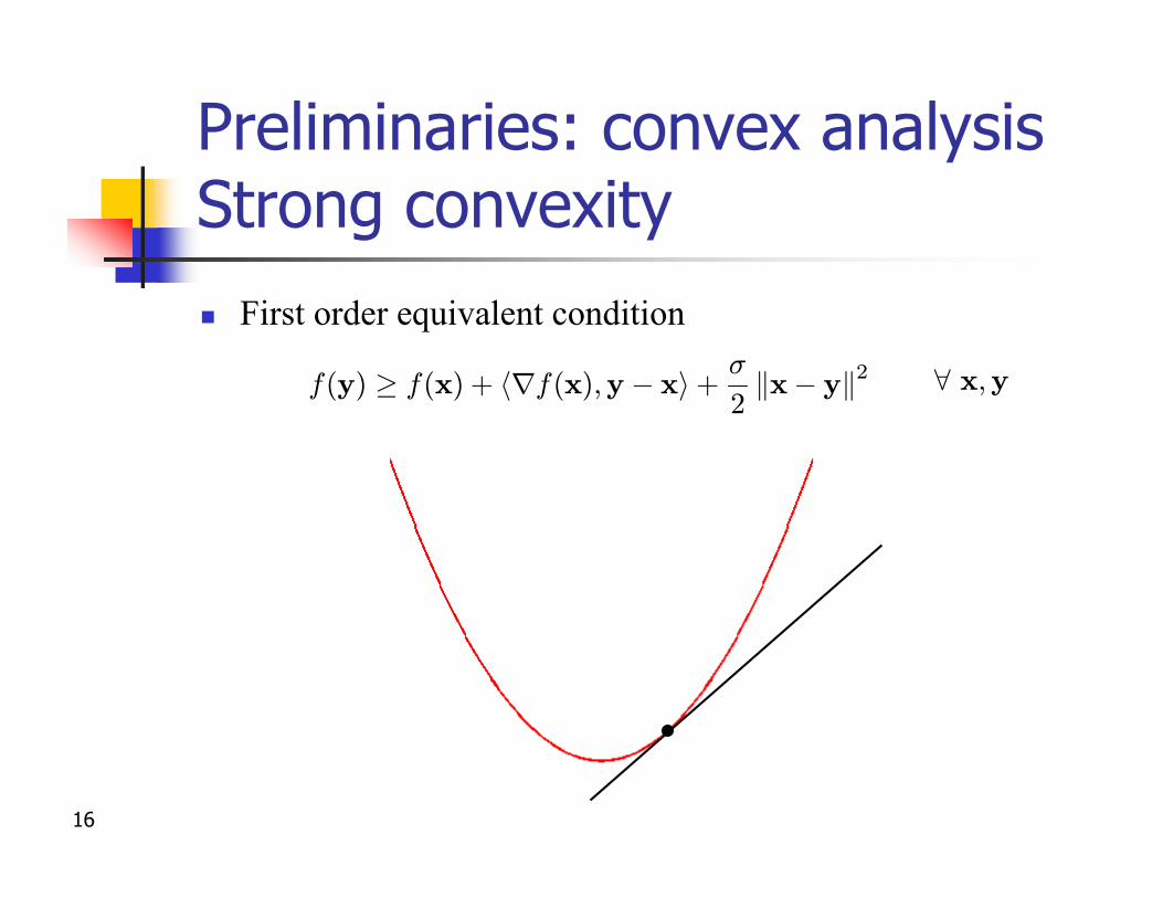
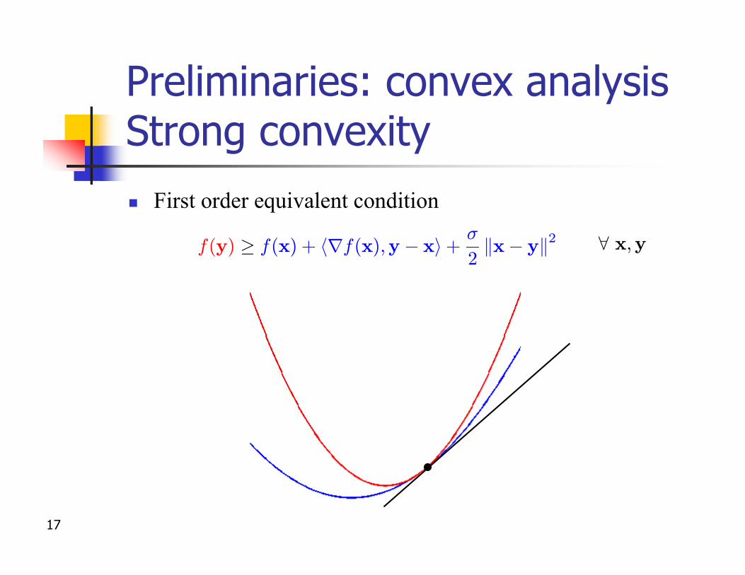
Preliminaries: convex analysisStrong convexityn First order equivalent condition
f(y) ¸ f(x) + hrf(x);y¡ xi +¾
2kx¡ yk2 8 x;y
17
Preliminaries: convex analysisStrong convexityn First order equivalent condition
8 x;yf(y) ¸ f(x) + hrf(x);y¡ xi +¾
2kx¡ yk2
18
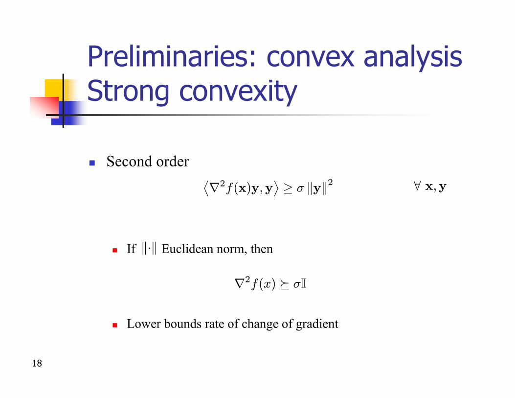
Preliminaries: convex analysisStrong convexity
n Second order
n If Euclidean norm, then
n Lower bounds rate of change of gradient
r2f(x)y;y
®¸ ¾ kyk2
r2f(x) º ¾I
k¢k
8 x;y
19
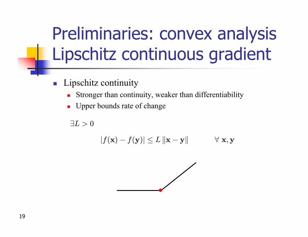
Preliminaries: convex analysisLipschitz continuous gradientn Lipschitz continuity
n Stronger than continuity, weaker than differentiabilityn Upper bounds rate of change
8 x;yjf(x)¡ f(y)j · L kx¡ yk
9L > 0
20
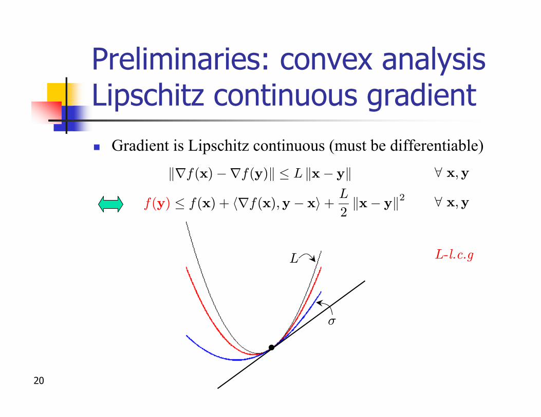
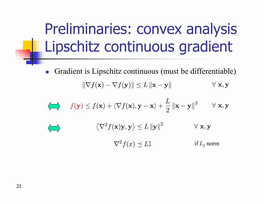
Preliminaries: convex analysisLipschitz continuous gradientn Gradient is Lipschitz continuous (must be differentiable)
8 x;yf(y) · f(x) + hrf(x);y¡ xi +L
2kx¡ yk2
8 x;ykrf(x)¡rf(y)k · L kx¡ yk
L-l.c.g
¾
L
21
Preliminaries: convex analysisLipschitz continuous gradientn Gradient is Lipschitz continuous (must be differentiable)
8 x;yf(y) · f(x) + hrf(x);y¡ xi +L
2kx¡ yk2
8 x;ykrf(x)¡rf(y)k · L kx¡ yk
8 x;yr2f(x)y;y
®· L kyk2
if L2 normr2f(x) ¹ LI
22
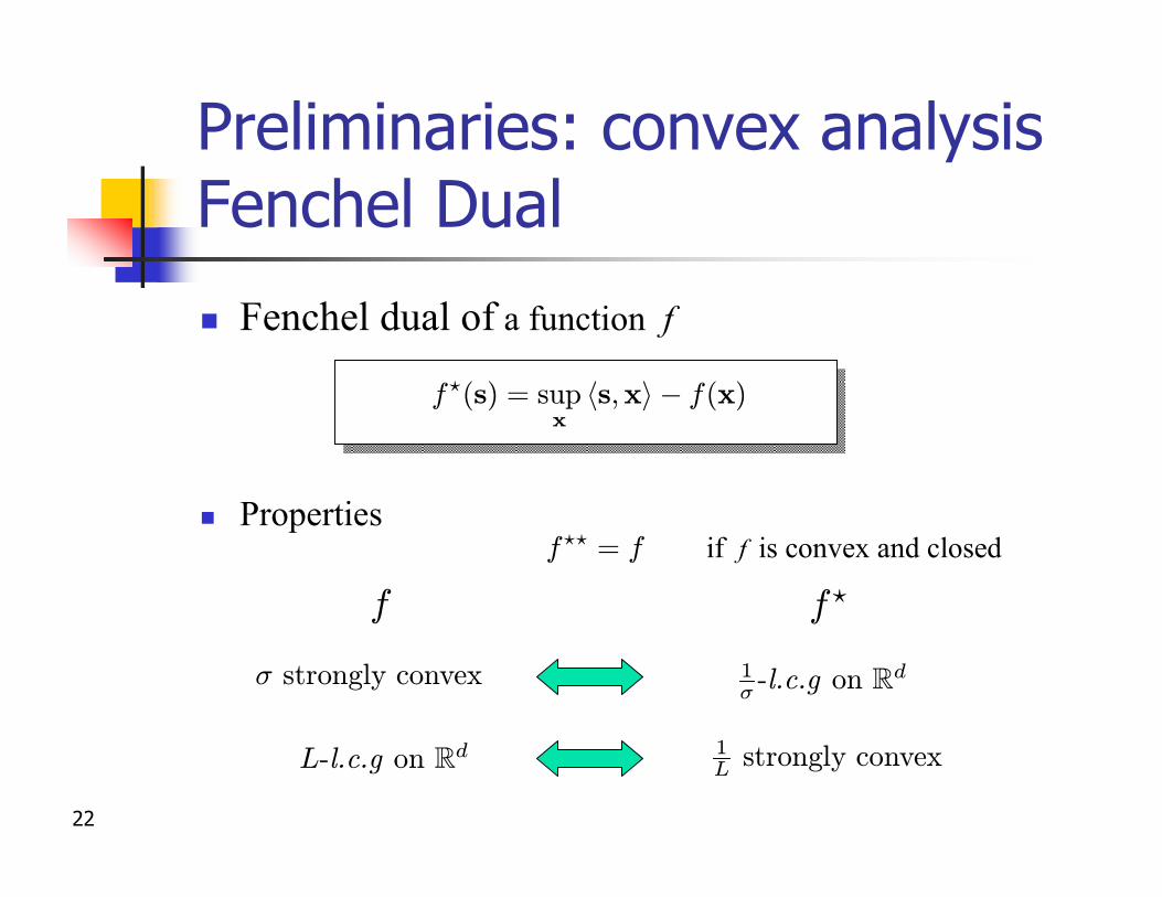
Preliminaries: convex analysis Fenchel Dual
n Fenchel dual of a function f
n Propertiesf?? = f
f?f
¾ strongly convex
1L strongly convex
f?(s) = supx
hs;xi¡ f(x)
L-l.c.g on Rd
1¾ -l.c.g on Rd
if f is convex and closed
23
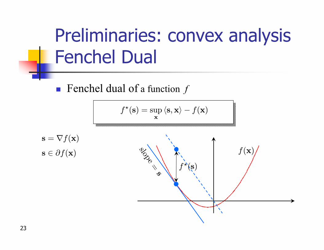
Preliminaries: convex analysis Fenchel Dual
n Fenchel dual of a function f
f?(s) = supx
hs;xi¡ f(x)
s 2 @f(x)
s = rf(x)
slope=
sf?(s)
f(x)
24
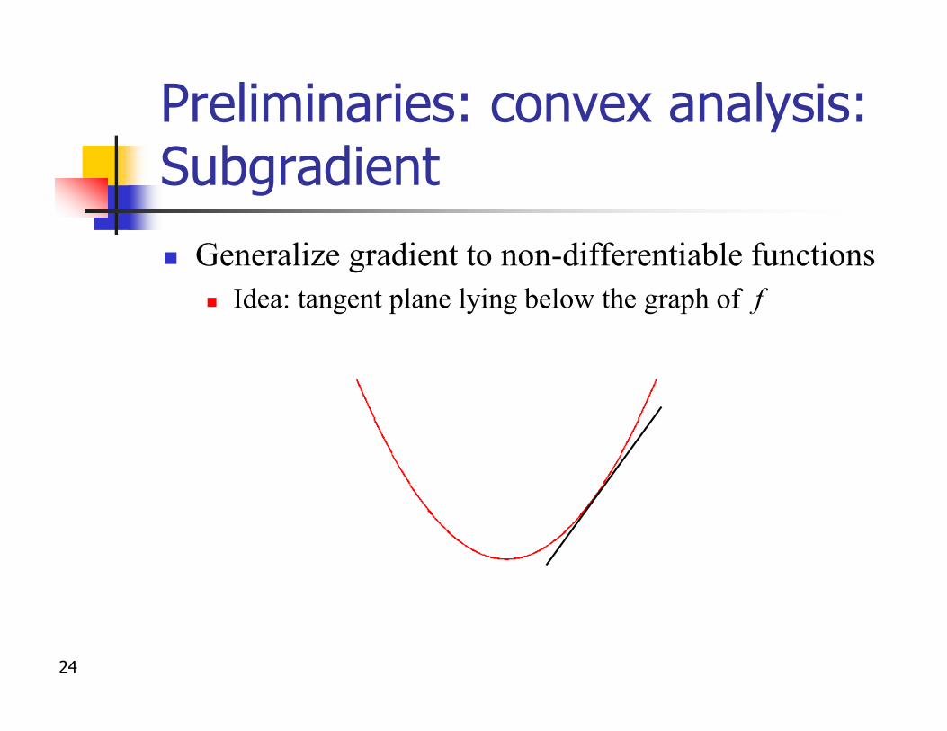
Preliminaries: convex analysis: Subgradientn Generalize gradient to non-differentiable functions
n Idea: tangent plane lying below the graph of f
25
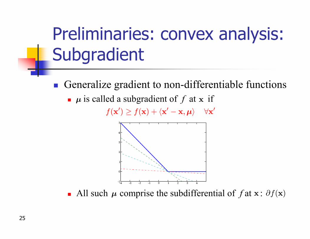
Preliminaries: convex analysis: Subgradient
n Generalize gradient to non-differentiable functionsn is called a subgradient of f at if
n All such comprise the subdifferential of f at :
¹
¹
f(x0) ¸ f(x) + hx0 ¡ x;¹i 8x0
@f(x)
x
x
26
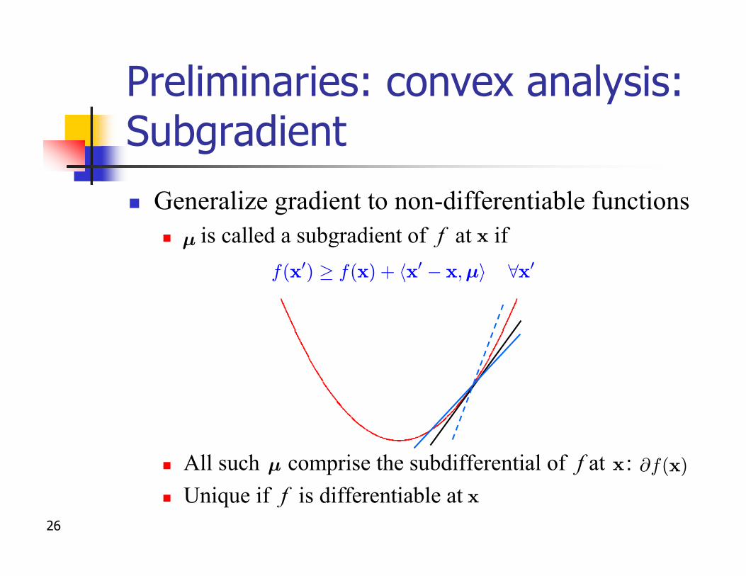
Preliminaries: convex analysis: Subgradientn Generalize gradient to non-differentiable functions
n is called a subgradient of f at if
n All such comprise the subdifferential of f at : n Unique if f is differentiable at
¹
¹
f(x0) ¸ f(x) + hx0 ¡ x;¹i 8x0
@f(x)
x
x
x
27
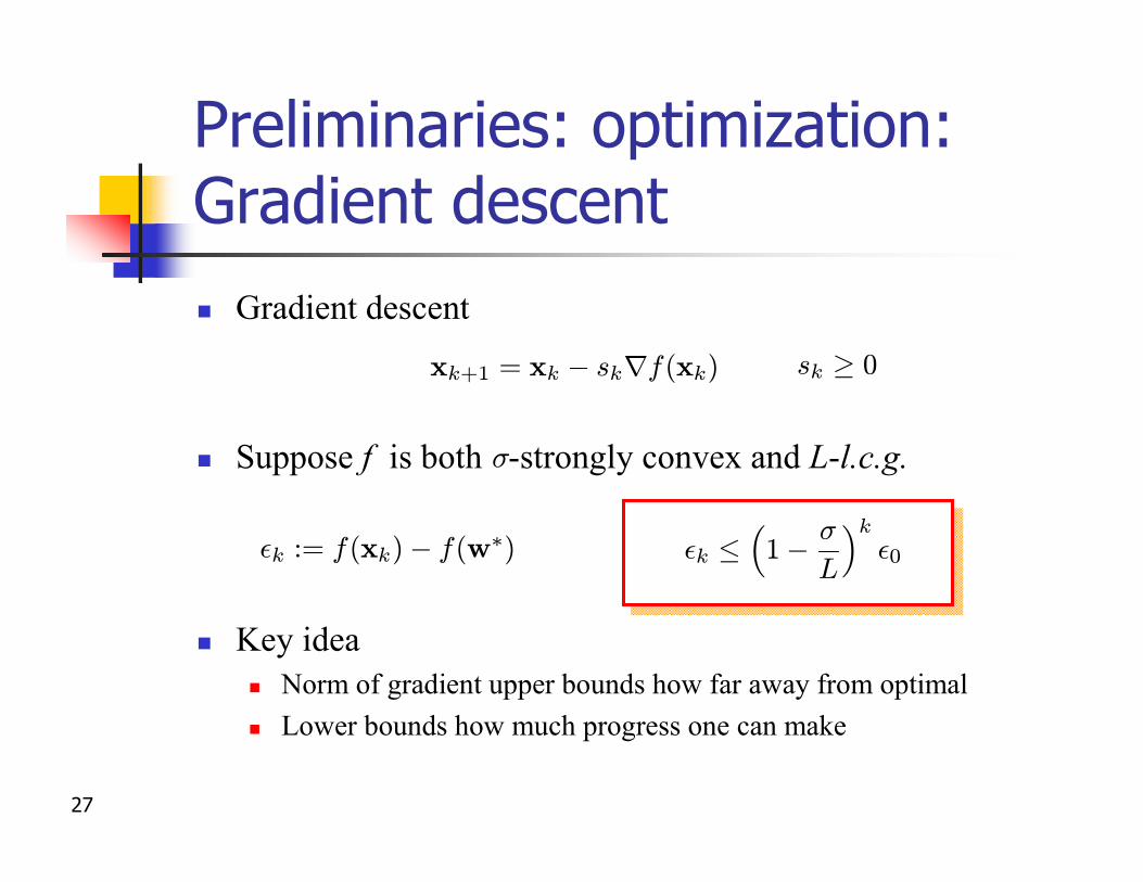
Preliminaries: optimization: Gradient descentn Gradient descent
n Suppose f is both -strongly convex and L-l.c.g.
n Key idean Norm of gradient upper bounds how far away from optimaln Lower bounds how much progress one can make
¾
xk+1 = xk ¡ skrf(xk) sk ¸ 0
²k := f(xk)¡ f(w¤) ²k ·³1¡ ¾
L
´k²0
28
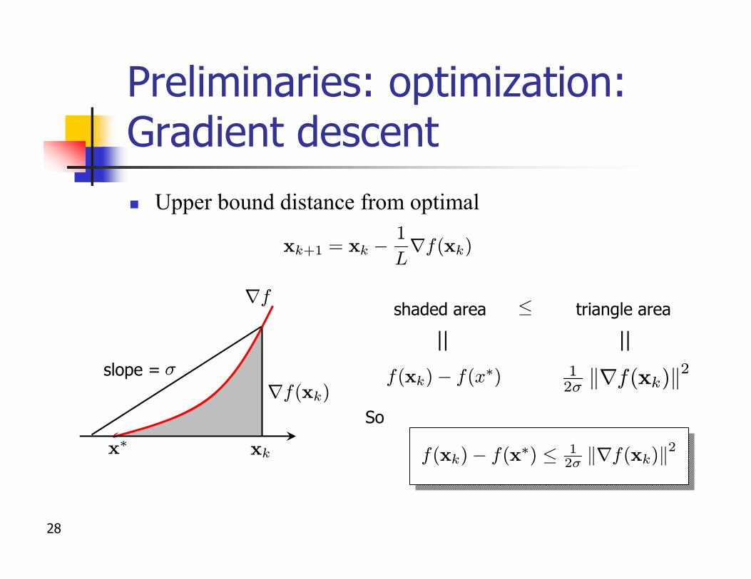
Preliminaries: optimization: Gradient descentn Upper bound distance from optimal
xk+1 = xk ¡1
Lrf(xk)
xk
slope = ¾
x¤
rf(xk)
shaded area triangle area·rf
f(xk)¡ f(x¤) 12¾ krf(xk)k2
So
f(xk)¡ f(x¤) · 12¾ krf(xk)k2
29
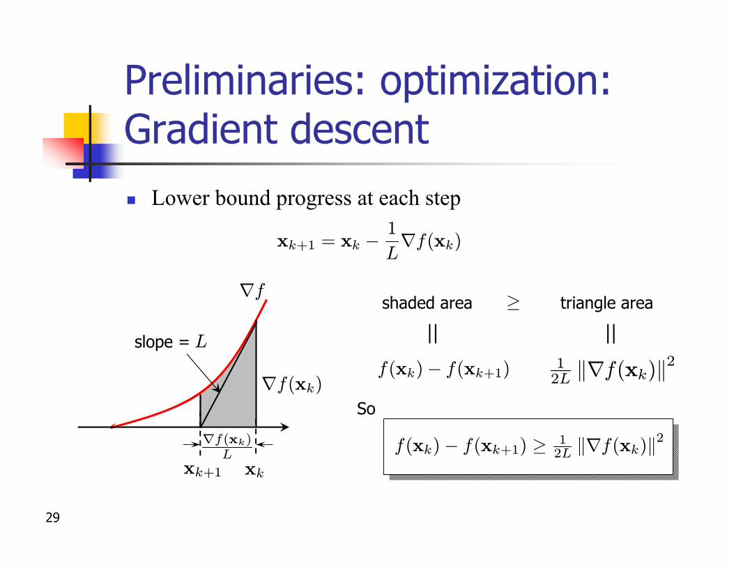
Preliminaries: optimization: Gradient descentn Lower bound progress at each step
xk+1 = xk ¡1
Lrf(xk)
xk
slope =
rf(xk)
shaded area triangle arearf
So
xk+1
L
¸
12L krf(xk)k2f(xk)¡ f(xk+1)
rf(xk)L
f(xk)¡ f(xk+1) ¸ 12L krf(xk)k2
30
Preliminaries: optimization: Gradient descent
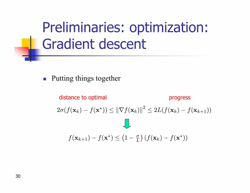
2¾(f(xk)¡ f(x¤)) · krf(xk)k2 · 2L(f(xk)¡ f(xk+1))
f(xk+1)¡ f(x¤) ·¡1¡ ¾
L
¢(f(xk)¡ f(x¤))
progressdistance to optimal
n Putting things together
31
Preliminaries: optimization: Gradient descent
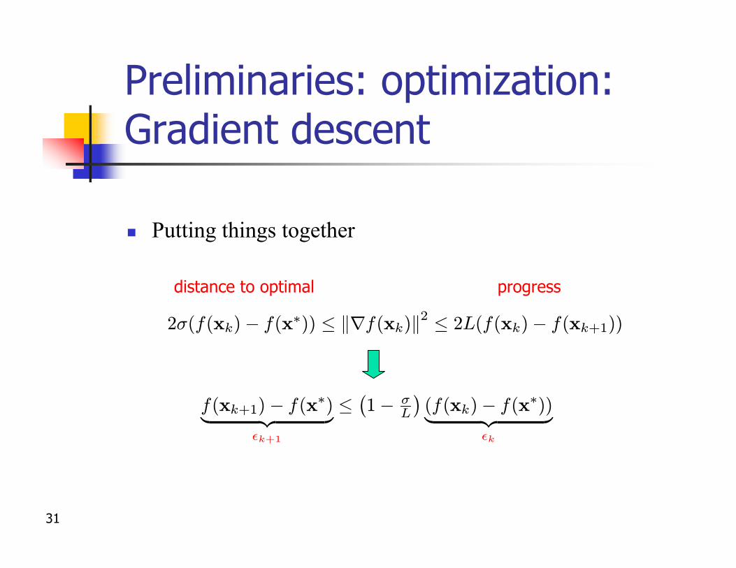
n Putting things together
2¾(f(xk)¡ f(x¤)) · krf(xk)k2 · 2L(f(xk)¡ f(xk+1))
f(xk+1)¡ f(x¤)| {z }²k+1
·¡1¡ ¾
L
¢(f(xk)¡ f(x¤))| {z }
²k
progressdistance to optimal
32
Preliminaries: optimization: Gradient descent
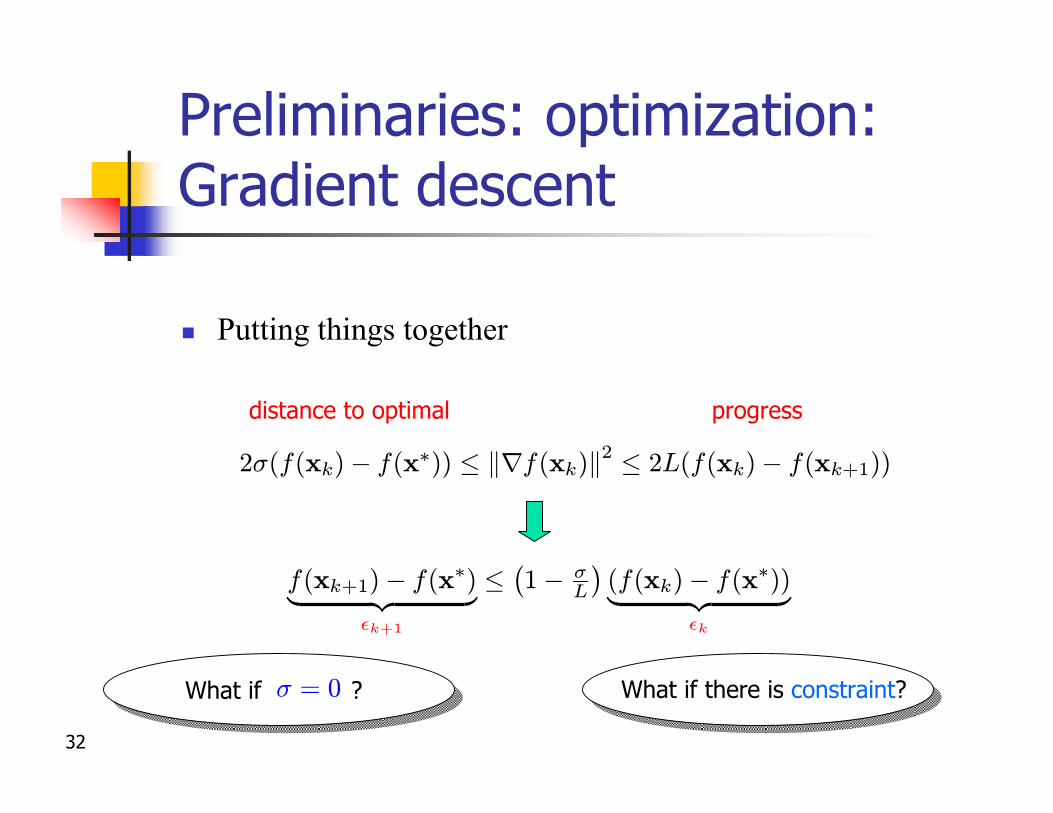
n Putting things together
2¾(f(xk)¡ f(x¤)) · krf(xk)k2 · 2L(f(xk)¡ f(xk+1))
f(xk+1)¡ f(x¤)| {z }²k+1
·¡1¡ ¾
L
¢(f(xk)¡ f(x¤))| {z }
²k
progressdistance to optimal
What if ?¾ = 0 What if there is constraint?
33
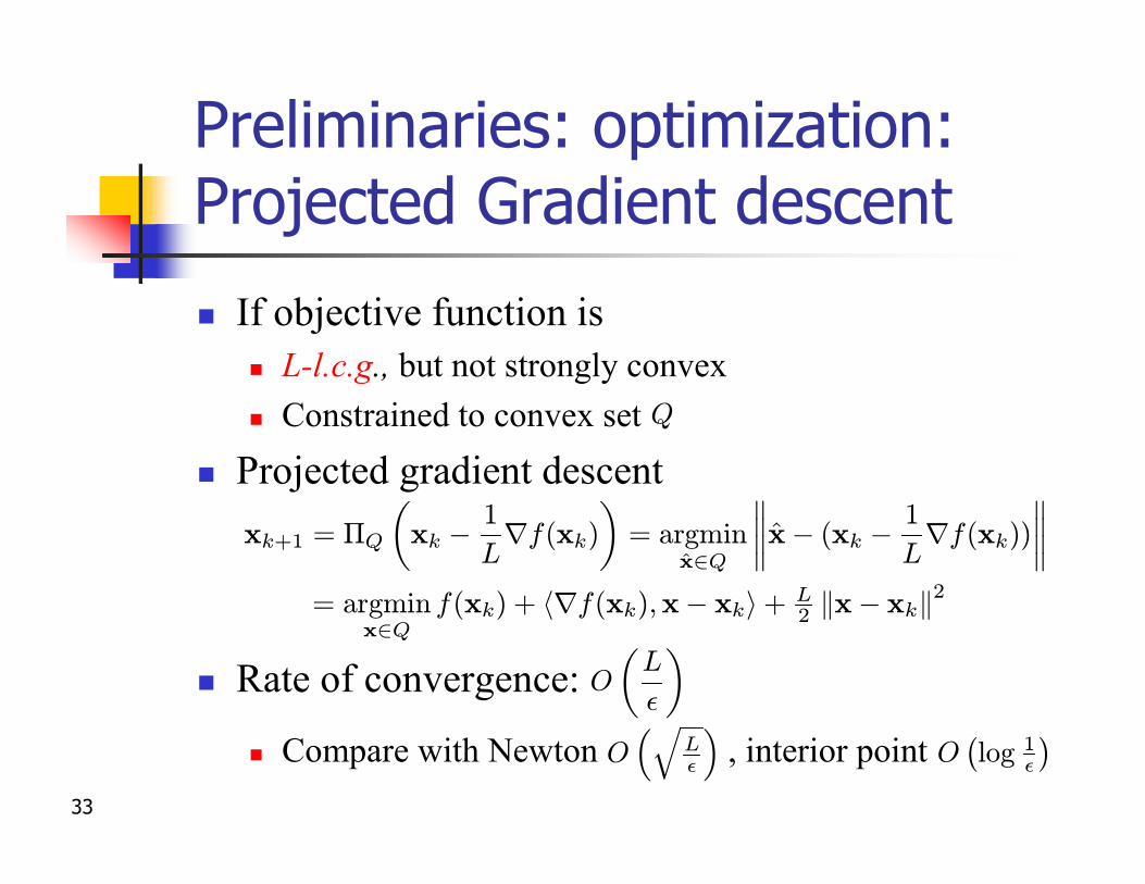
Preliminaries: optimization: Projected Gradient descent
n If objective function isn L-l.c.g., but not strongly convexn Constrained to convex set
n Projected gradient descent
n Rate of convergence:
n Compare with Newton , interior point
O
µL
²
Q
= argminx2Q
f(xk) + hrf(xk);x¡ xki + L2 kx¡ xkk2
O¡log 1
²
¢
xk+1 = ¦Q
µxk ¡
1
Lrf(xk)
¶= argmin
x̂2Q
°°°°x̂¡ (xk ¡1
Lrf(xk))
°°°°
O³q
L²
´
34
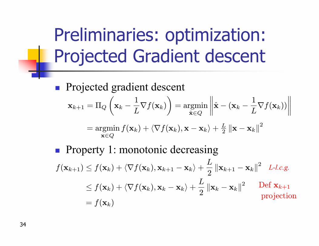
Preliminaries: optimization: Projected Gradient descent
n Projected gradient descent
n Property 1: monotonic decreasing
= argminx2Q
f(xk) + hrf(xk);x¡ xki + L2 kx¡ xkk2
f(xk+1) · f(xk) + hrf(xk);xk+1 ¡ xki +L
2kxk+1 ¡ xkk2
· f(xk) + hrf(xk);xk ¡ xki +L
2kxk ¡ xkk2
= f(xk)
L-l.c.g.
Def xk+1
xk+1 = ¦Q
µxk ¡
1
Lrf(xk)
¶= argmin
x̂2Q
°°°°x̂¡ (xk ¡1
Lrf(xk))
°°°°
projection
35
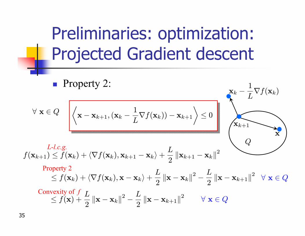
Preliminaries: optimization: Projected Gradient descent
n Property 2:
¿x¡ xk+1; (xk ¡
1
Lrf(xk))¡ xk+1
À· 0
xk ¡1
Lrf(xk)
xk+1
xQ
8 x 2 Q
f(xk+1) · f(xk) + hrf(xk);xk+1 ¡ xki +L
2kxk+1 ¡ xkk2
· f(xk) + hrf(xk);x¡ xki +L
2kx¡ xkk2 ¡ L
2kx¡ xk+1k2
· f(x) +L
2kx¡ xkk2 ¡ L
2kx¡ xk+1k2
L-l.c.g.
Property 2
Convexity of f
8 x 2 Q
8 x 2 Q
36
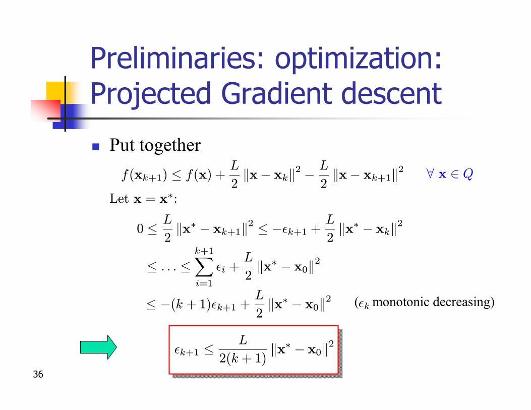
Preliminaries: optimization: Projected Gradient descent
n Put togetherf(xk+1) · f(x) +
L
2kx¡ xkk2 ¡ L
2kx¡ xk+1k2 8 x 2 Q
0 · L
2kx¤ ¡ xk+1k2 · ¡²k+1 +
L
2kx¤ ¡ xkk2
· : : : ·k+1X
i=1
²i +L
2kx¤ ¡ x0k2
· ¡(k + 1)²k+1 +L
2kx¤ ¡ x0k2
²k+1 ·L
2(k + 1)kx¤ ¡ x0k2
( monotonic decreasing)²k
Let x = x¤:
37
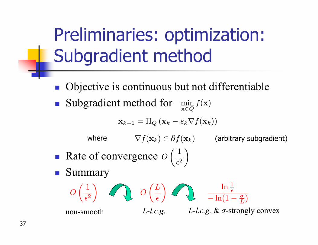
Preliminaries: optimization: Subgradient method
n Objective is continuous but not differentiablen Subgradient method for
n Rate of convergencen Summary
xk+1 = ¦Q (xk ¡ skrf(xk))
where
minx2Q
f(x)
rf(xk) 2 @f(xk) (arbitrary subgradient)
O
µ1
²2
non-smooth L-l.c.g. L-l.c.g. & -strongly convex¾
O
µ1
²2
¶O
µL
²
¶ln 1
²
¡ ln(1¡ ¾L)
38
Outlinen The problem from machine learning perspectiven Preliminaries
n Convex analysis and gradient descentn Nesterov’s optimal gradient method
n Lower bound of optimizationn Optimal gradient method
n Utilizing structure: composite optimizationn Smooth minimizationn Excessive gap minimization
n Conclusion
39
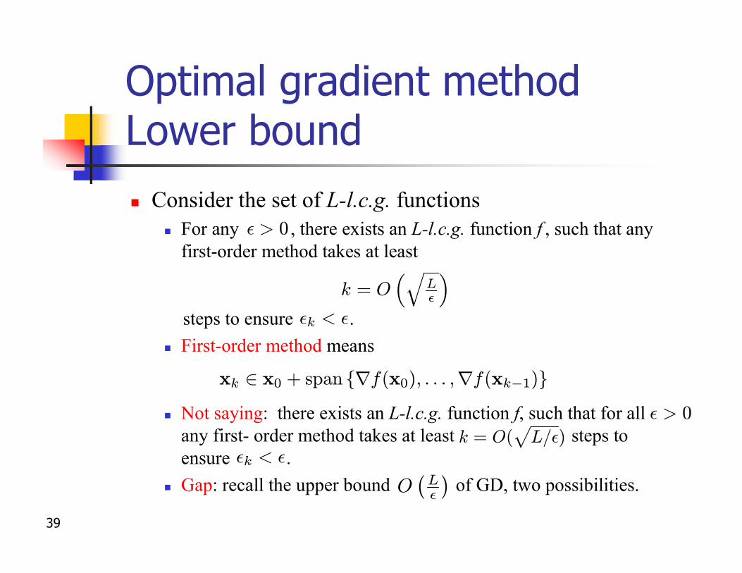
Optimal gradient method Lower boundn Consider the set of L-l.c.g. functions
n For any , there exists an L-l.c.g. function f , such that any first-order method takes at least
steps to ensure .n First-order method means
n Not saying: there exists an L-l.c.g. function f, such that for all any first- order method takes at least steps to ensure .
n Gap: recall the upper bound of GD, two possibilities.
²k < ²
² > 0
xk 2 x0 + span frf(x0); : : : ; rf(xk¡1)g
k = O(p
L=²)²k < ²
O¡L²
¢
k = O³q
L²
´
² > 0
40
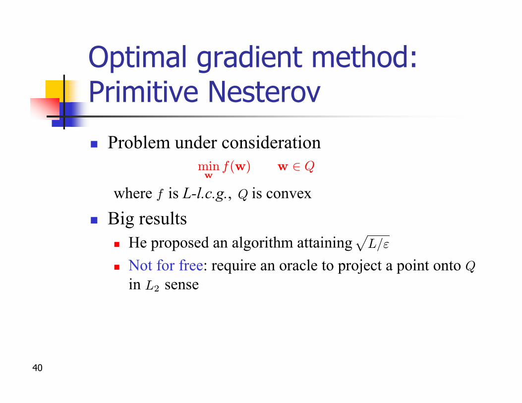
Optimal gradient method: Primitive Nesterov
n Problem under consideration
where is L-l.c.g., is convex
n Big results n He proposed an algorithm attaining n Not for free: require an oracle to project a point onto
in senseL2
Q
Q
f
minw
f(w) w 2 Q
pL="
41
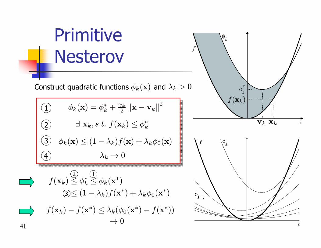
Primitive Nesterov
¸k ! 0
Construct quadratic functions and Ák(x) ¸k > 0
f(xk)
vk xk
! 0
f(xk)¡ f(x¤) · ¸k(Á0(x¤)¡ f(x¤))
Ák(x) · (1¡ ¸k)f(x) + ¸kÁ0(x)
1
9 xk; s:t: f(xk) · Á¤k2
3
2 1f(xk) · Á¤k · Ák(x
¤)
· (1¡ ¸k)f(x¤) + ¸kÁ0(x¤)
4
3
Ák(x) = Á¤k + °k2 kx¡ vkk2
42
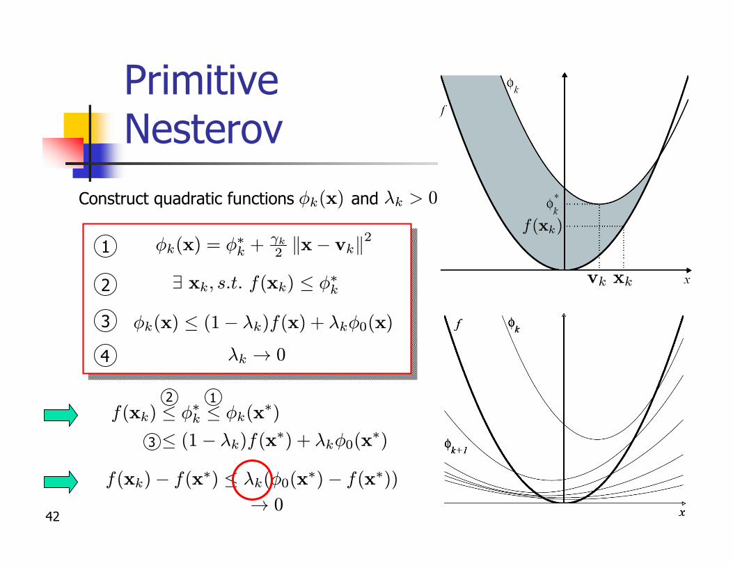
Primitive Nesterov
¸k ! 0
Construct quadratic functions and Ák(x) ¸k > 0
! 0
f(xk)¡ f(x¤) · ¸k(Á0(x¤)¡ f(x¤))
Ák(x) · (1¡ ¸k)f(x) + ¸kÁ0(x)
1
9 xk; s:t: f(xk) · Á¤k2
3
2 1f(xk) · Á¤k · Ák(x
¤)
· (1¡ ¸k)f(x¤) + ¸kÁ0(x¤)
4
3
vk xk
f(xk)Ák(x) = Á¤k + °k
2 kx¡ vkk2
43
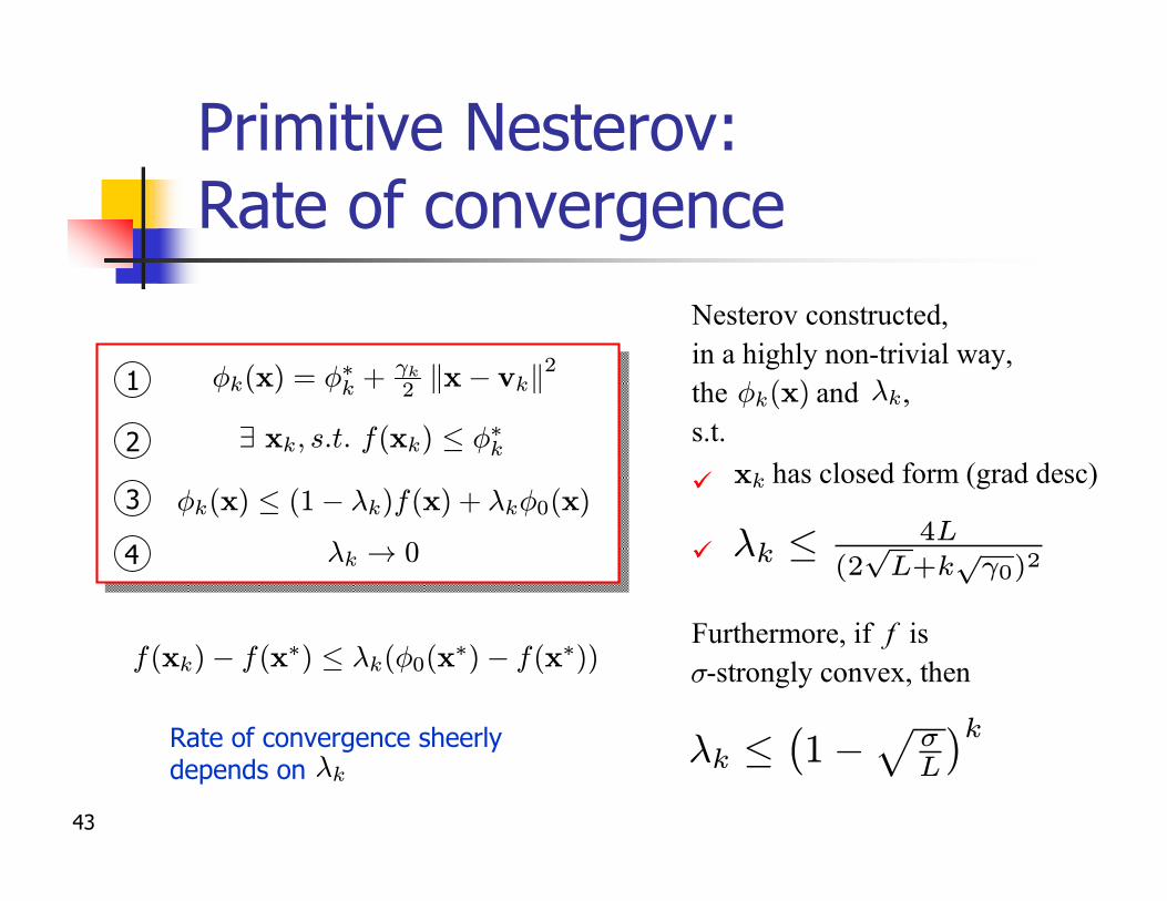
Primitive Nesterov:Rate of convergence
¸k ! 0
Ák(x) · (1¡ ¸k)f(x) + ¸kÁ0(x)
1
9 xk; s:t: f(xk) · Á¤k2
3
4
f(xk)¡ f(x¤) · ¸k(Á0(x¤)¡ f(x¤))
Rate of convergence sheerlydepends on ¸k
Nesterov constructed, in a highly non-trivial way,the and ,s.t.
Ák(x) ¸k
Furthermore, if f is -strongly convex, then¾
¸k · 1 ¡ ¾L
k
has closed form (grad desc)xkü
ü
Ák(x) = Á¤k + °k2 kx¡ vkk2
¸k · 4L(2pL+k
p°0)2
44
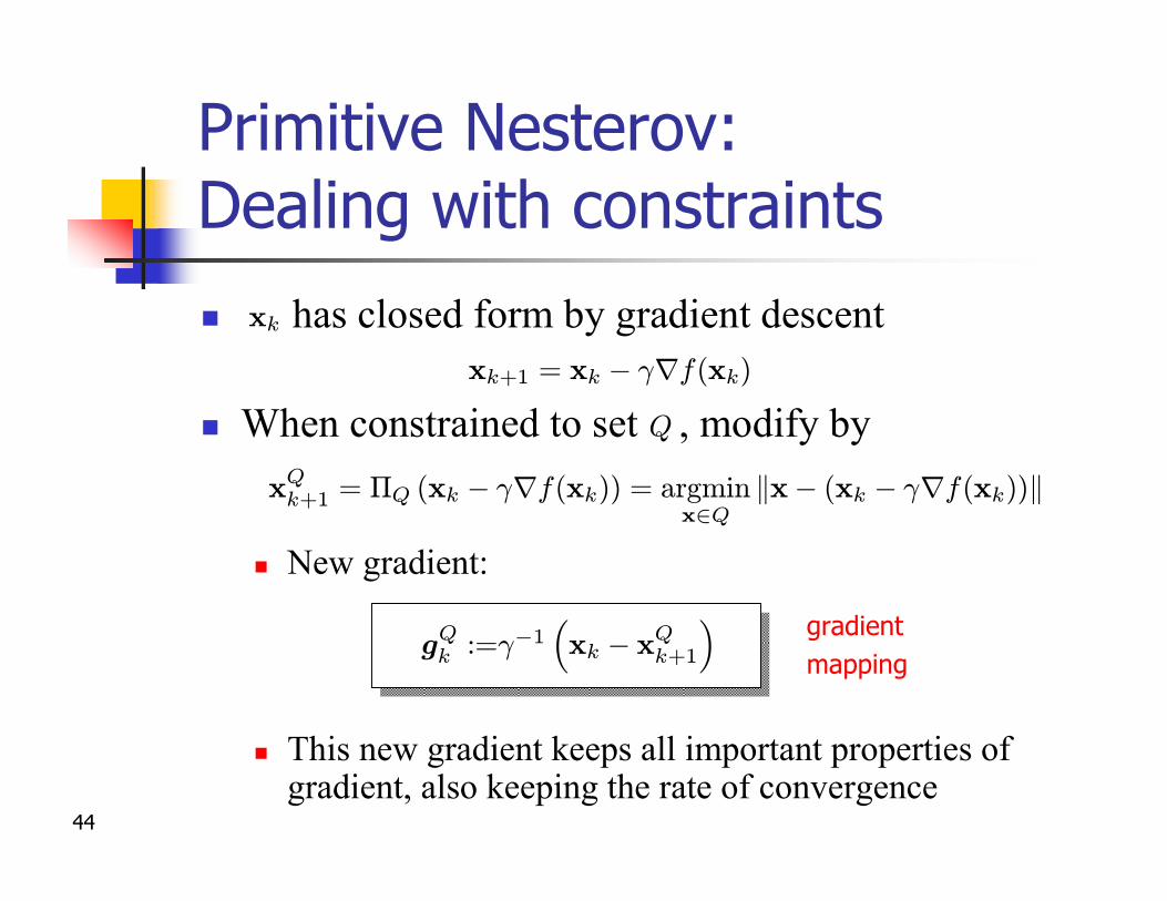
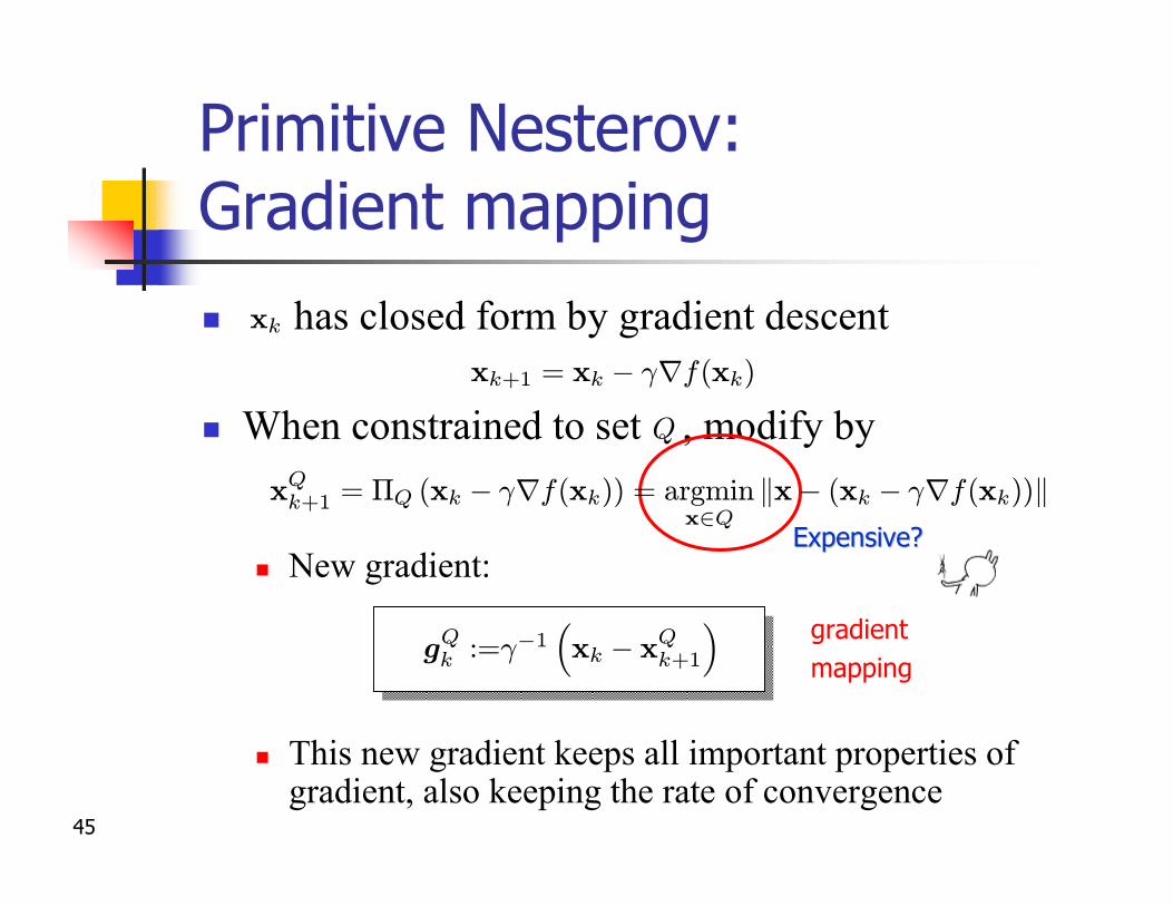
Primitive Nesterov:Dealing with constraintsn has closed form by gradient descent
n When constrained to set , modify by
n New gradient:
n This new gradient keeps all important properties of gradient, also keeping the rate of convergence
Q
xk
gradientmapping
xQk+1 = ¦Q (xk ¡ °rf(xk)) = argminx2Q
kx¡ (xk ¡ °rf(xk))k
gQk :=°¡1³xk ¡ xQk+1
´
xk+1 = xk ¡ °rf(xk)
45
Primitive Nesterov:Gradient mappingn has closed form by gradient descent
n When constrained to set , modify by
n New gradient:
n This new gradient keeps all important properties of gradient, also keeping the rate of convergence
Q
xk
gradientmapping
Expensive?Expensive?
xQk+1 = ¦Q (xk ¡ °rf(xk)) = argminx2Q
kx¡ (xk ¡ °rf(xk))k
gQk :=°¡1³xk ¡ xQk+1
´
xk+1 = xk ¡ °rf(xk)
46
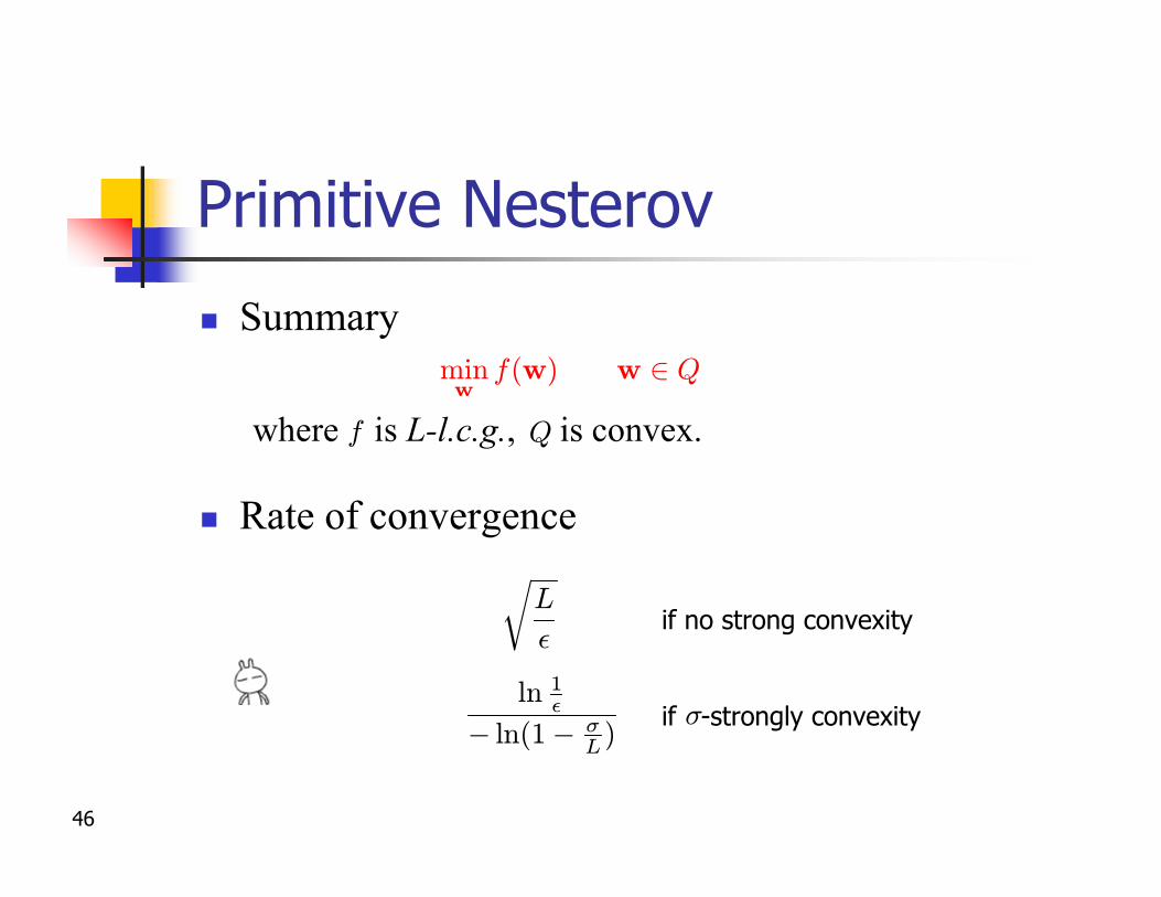
Primitive Nesterov
n Summary
where is L-l.c.g., is convex.
n Rate of convergence
Qf
minw
f(w) w 2 Q
rL
²if no strong convexity
ln 1²
¡ ln(1¡ ¾L)
if -strongly convexity¾
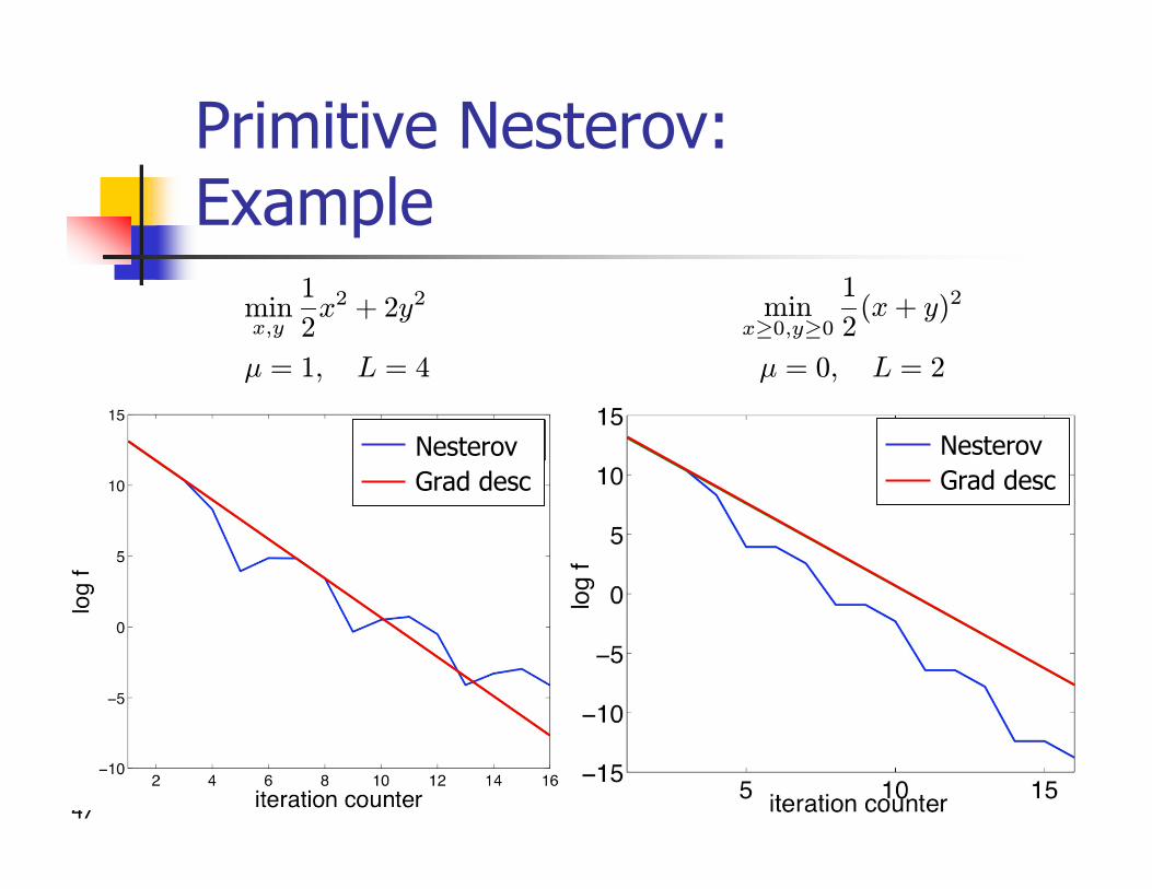
47
Primitive Nesterov: Example
minx;y
1
2x2 + 2y2
¹ = 1; L = 4
minx¸0;y¸0
1
2(x + y)2
¹ = 0; L = 2
NesterovGrad desc
NesterovGrad desc
48
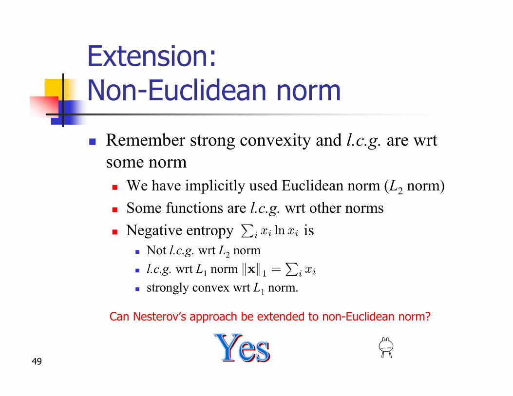
Extension:Non-Euclidean norm
n Remember strong convexity and l.c.g. are wrtsome normn We have implicitly used Euclidean norm (L2 norm)n Some functions are strongly convex wrt other normsn Negative entropy is
n Not l.c.g. wrt L2 normn l.c.g. wrt L1 normn strongly convex wrt L1 norm.
kxk1 =P
i xi
Pi xi ln xi
Can Nesterov’s approach be extended to non-Euclidean norm?
49
Extension:Non-Euclidean norm
n Remember strong convexity and l.c.g. are wrtsome normn We have implicitly used Euclidean norm (L2 norm)n Some functions are l.c.g. wrt other normsn Negative entropy is
n Not l.c.g. wrt L2 normn l.c.g. wrt L1 normn strongly convex wrt L1 norm.
kxk1 =P
i xi
Pi xi ln xi
Can Nesterov’s approach be extended to non-Euclidean norm?
50
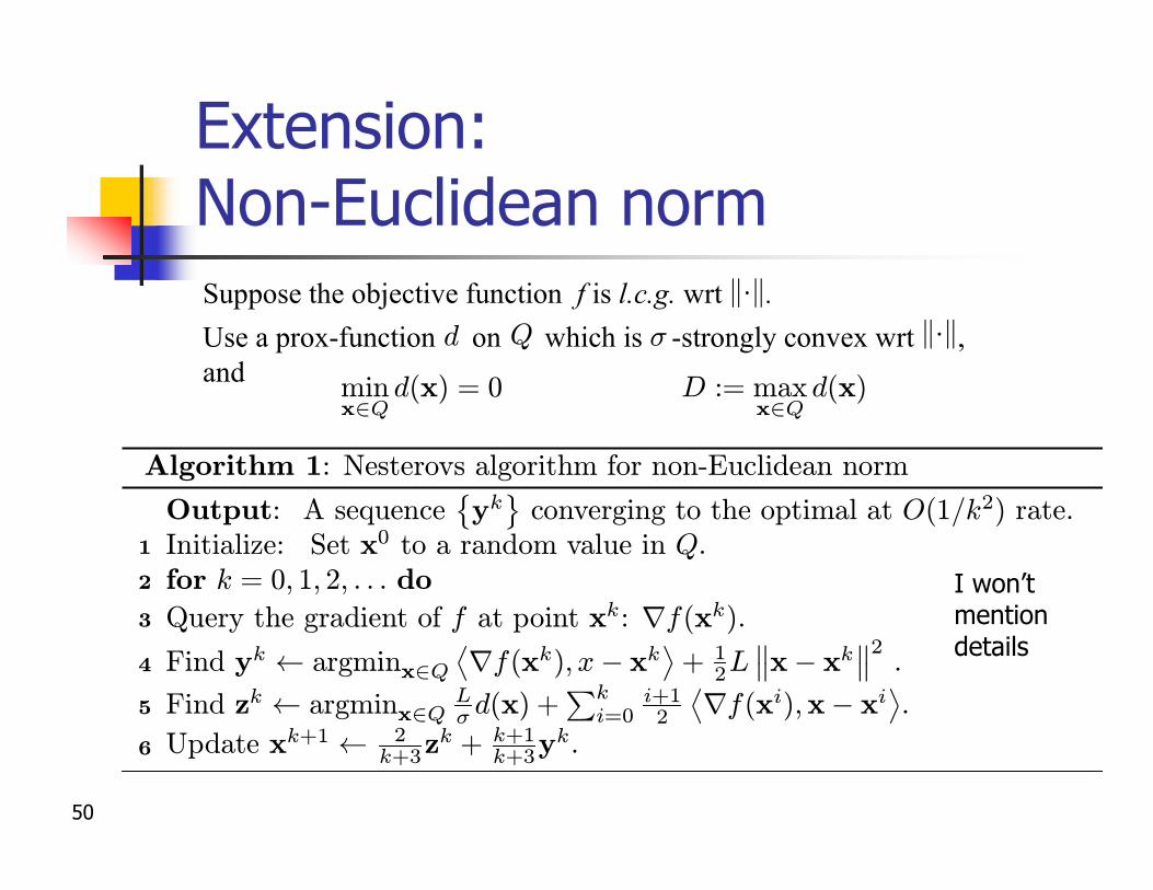
Extension:Non-Euclidean norm
I won’t mention details
Use a prox-function on which is -strongly convex wrt , and
k¢kQd
minx2Q
d(x) = 0 D := maxx2Q
d(x)
Suppose the objective function f is l.c.g. wrt .k¢k¾
Algorithm 1: Nesterovs algorithm for non-Euclidean norm
Output: A sequence©ykª
converging to the optimal at O(1=k2) rate.Initialize: Set x0 to a random value in Q.1
for k = 0; 1; 2; : : : do2
Query the gradient of f at point xk: rf(xk).3
Find yk à argminx2Qrf(xk); x¡ xk
®+ 1
2L°°x¡ xk
°°2.4
Find zk à argminx2QL¾ d(x) +
Pki=0
i+12
rf(xi);x¡ xi
®.5
Update xk+1 Ã 2k+3z
k + k+1k+3y
k.6
51
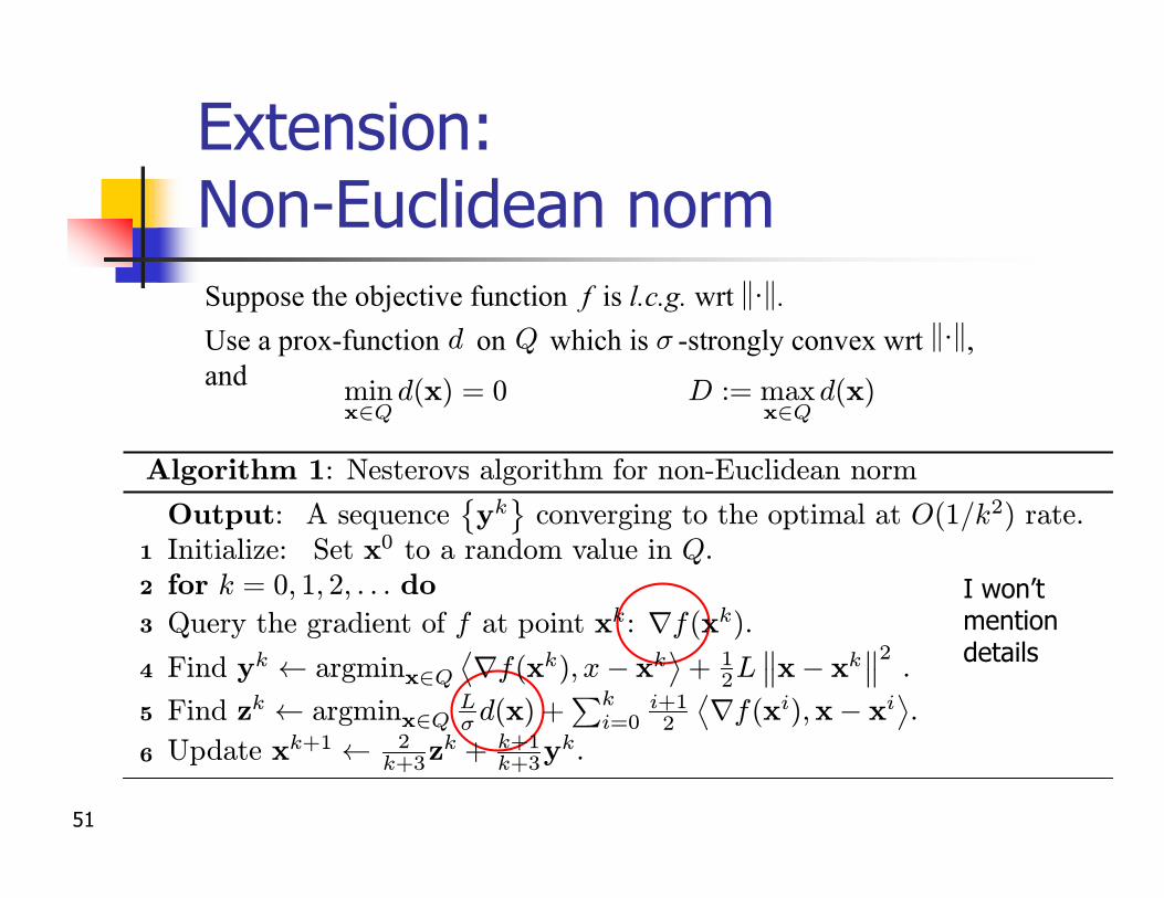
Extension:Non-Euclidean norm
I won’t mention details
Use a prox-function on which is -strongly convex wrt , and
k¢kQd
minx2Q
d(x) = 0 D := maxx2Q
d(x)
Suppose the objective function f is l.c.g. wrt .k¢k¾
Algorithm 1: Nesterovs algorithm for non-Euclidean norm
Output: A sequence©ykª
converging to the optimal at O(1=k2) rate.Initialize: Set x0 to a random value in Q.1
for k = 0; 1; 2; : : : do2
Query the gradient of f at point xk: rf(xk).3
Find yk à argminx2Qrf(xk); x¡ xk
®+ 1
2L°°x¡ xk
°°2.4
Find zk à argminx2QL¾ d(x) +
Pki=0
i+12
rf(xi);x¡ xi
®.5
Update xk+1 Ã 2k+3z
k + k+1k+3y
k.6
52
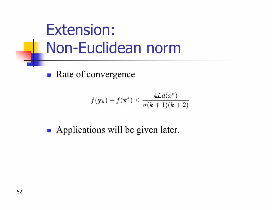
Extension:Non-Euclidean norm
n Rate of convergence
n Applications will be given later.
f(yk)¡ f(x¤) · 4Ld(x¤)¾(k + 1)(k + 2)
53
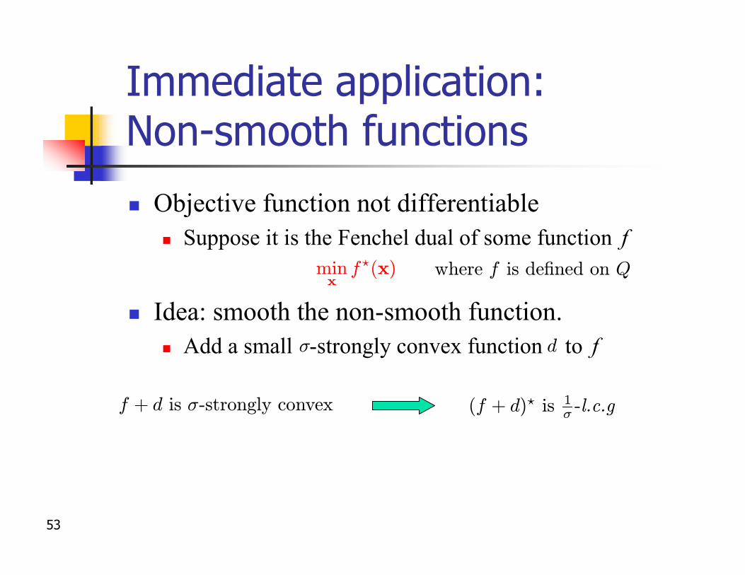
Immediate application:Non-smooth functions
n Objective function not differentiablen Suppose it is the Fenchel dual of some function f
n Idea: smooth the non-smooth function. n Add a small -strongly convex function to fd
minx
f?(x) where f is de¯ned on Q
¾
f + d is ¾-strongly convex (f + d)? is 1¾ -l.c.g
54
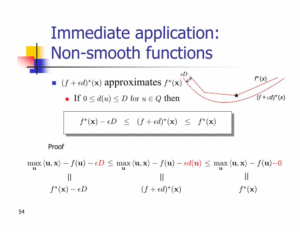
Immediate application:Non-smooth functions
n approximatesn If then0 · d(u) · D for u 2 Q
· ·
(f + ²d)?(x) f?(x)f?(x)¡ ²D
= ==
f?(x)(f + ²d)?(x)
(f + ²d)?(x)f?(x)¡ ²D f?(x)· ·
Proof
maxu
hu;xi¡ f(u)¡ ²D maxu
hu;xi¡ f(u)¡ ²d(u) maxu
hu;xi¡ f(u)¡0
55
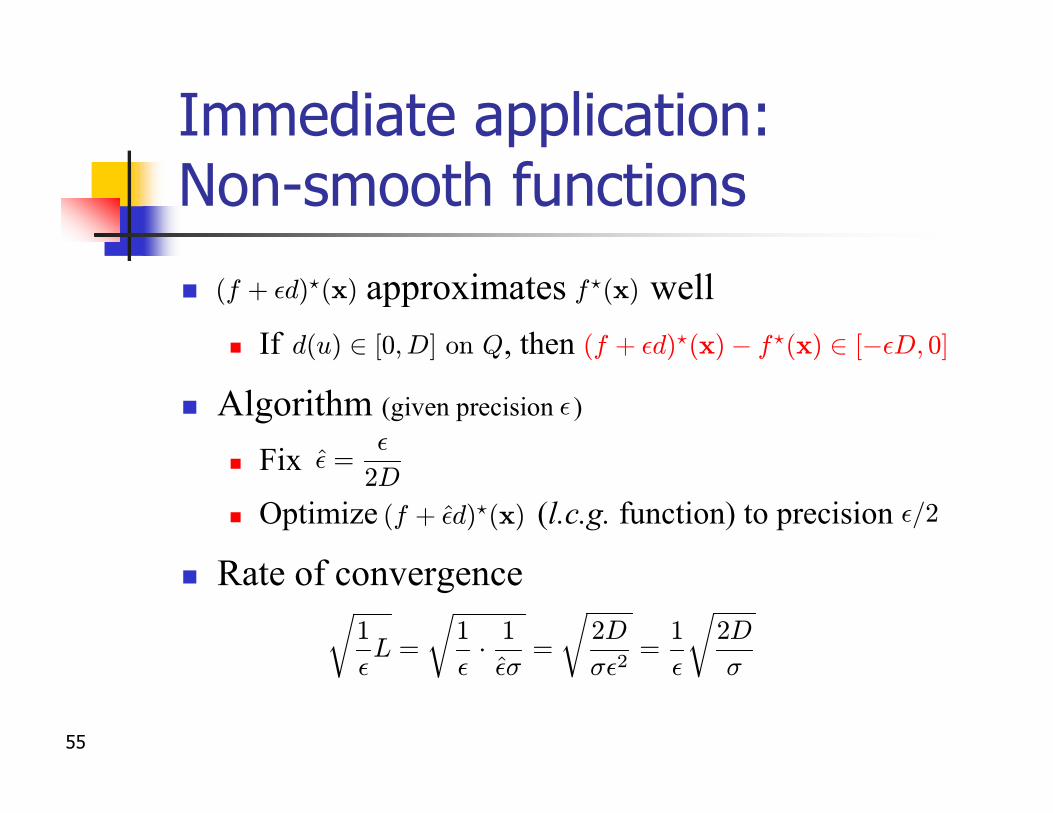
Immediate application:Non-smooth functions
n approximates well n If , then
n Algorithm (given precision )
n Fix
n Optimize (l.c.g. function) to precision
n Rate of convergence
f?(x)(f + ²d)?(x)
²
²̂ =²
2D
(f + ²̂d)?(x) ²=2
d(u) 2 [0; D] on Q
r1
²L =
r1
²¢ 1
²̂¾=
r2D
¾²2=
1
²
r2D
¾
(f + ²d)?(x)¡ f?(x) 2 [¡²D; 0]
56
Outlinen The problem from machine learning perspectiven Preliminaries
n Convex analysis and gradient descentn Nesterov’s optimal gradient method
n Lower bound of optimizationn Optimal gradient method
n Utilizing structure: composite optimizationn Smooth minimizationn Excessive gap minimization
n Conclusion
57
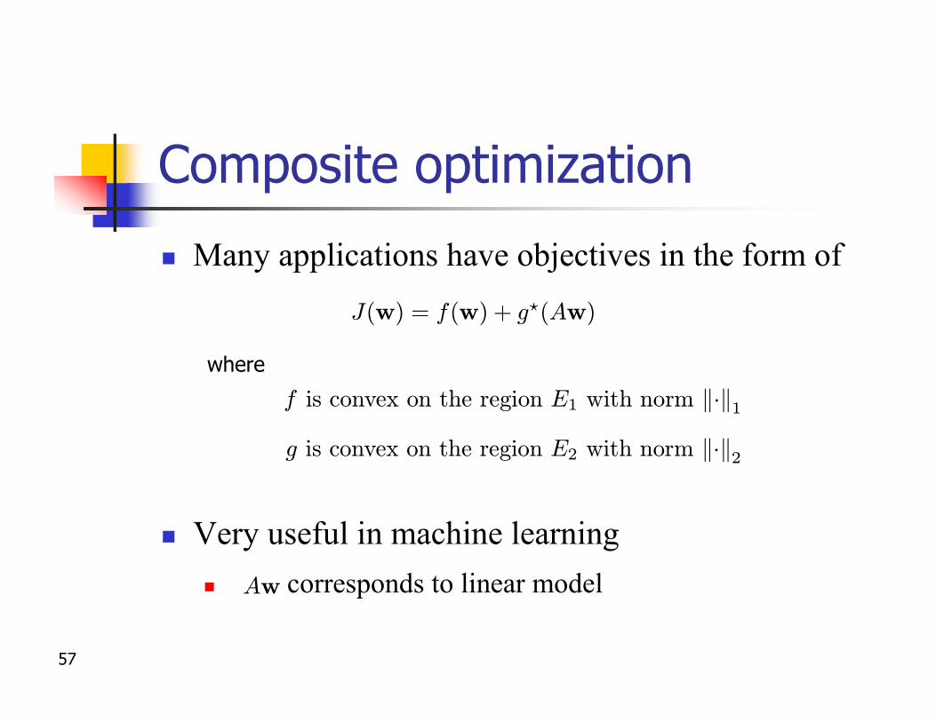
Composite optimization
n Many applications have objectives in the form of
n Very useful in machine learning n corresponds to linear model
J(w) = f(w) + g?(Aw)
where
f is convex on the region E1 with norm k¢k1
g is convex on the region E2 with norm k¢k2
Aw
58
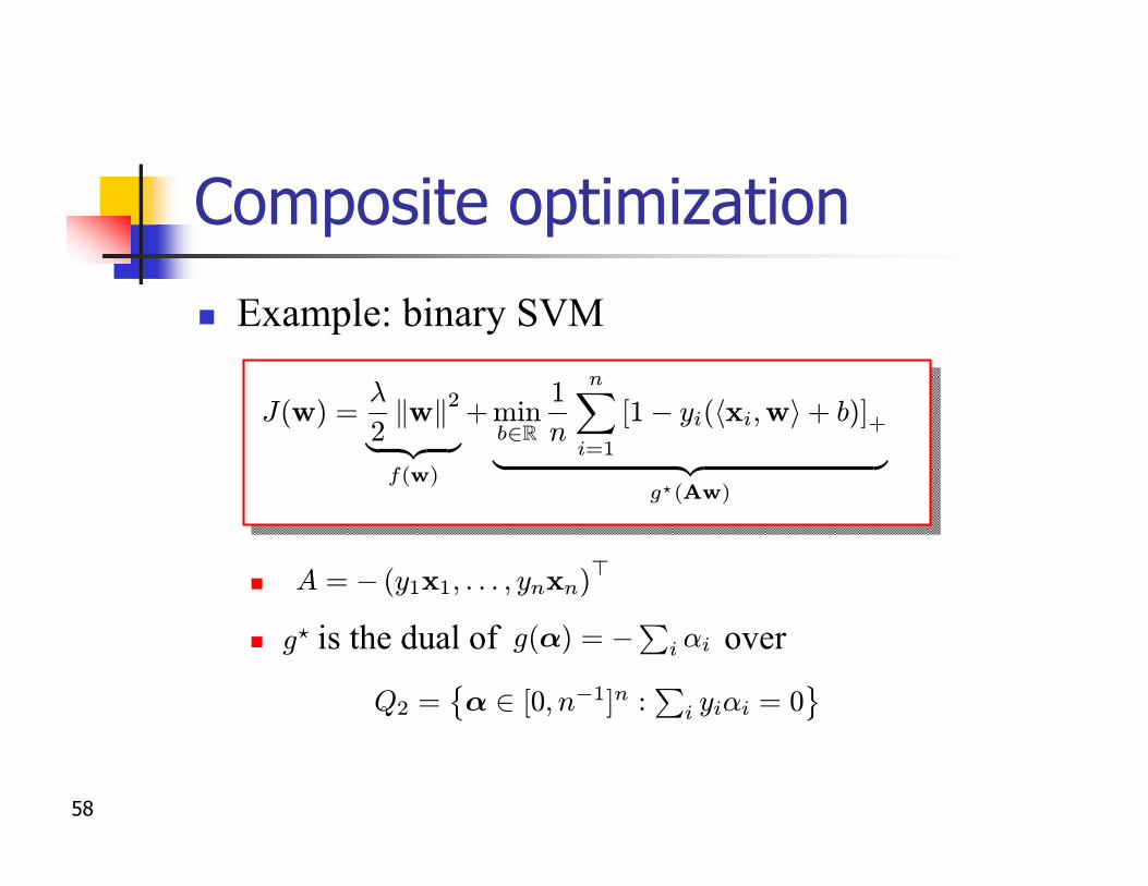
Composite optimization
n Example: binary SVM
n
n is the dual of overg? g(®) = ¡Pi ®i
A = ¡ (y1x1; : : : ; ynxn)>
Q2 =©® 2 [0; n¡1]n :
Pi yi®i = 0
ª
J(w) =¸
2kwk2
| {z }f(w)
+minb2R
1
n
nX
i=1
[1¡ yi(hxi;wi + b)]+
| {z }g?(Aw)
59
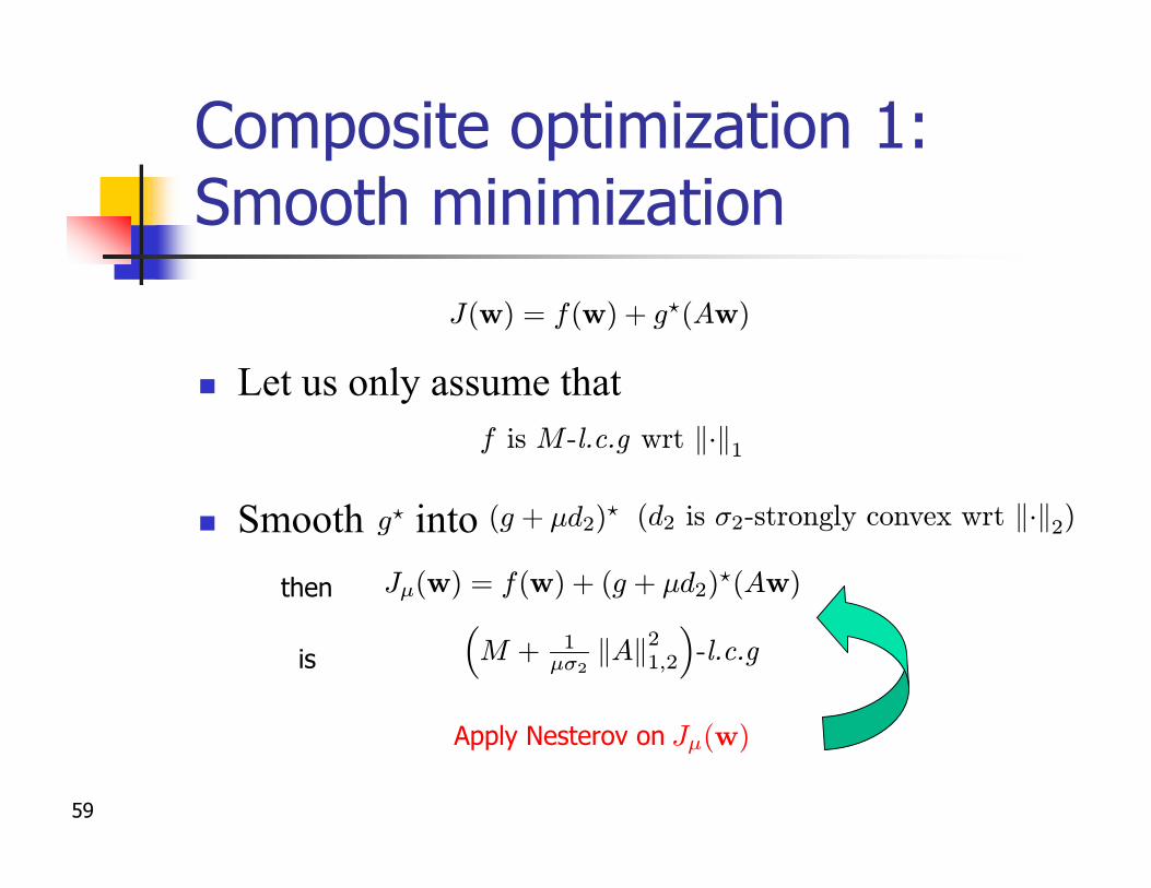
Composite optimization 1:Smooth minimization
n Let us only assume that
n Smooth into
J(w) = f(w) + g?(Aw)
f is M -l.c.g wrt k¢k1
g? (g + ¹d2)?
J¹(w) = f(w) + (g + ¹d2)?(Aw)
is
Apply Nesterov on J¹(w)
then
(d2 is ¾2-strongly convex wrt k¢k2)
³M + 1
¹¾2kAk2
1;2
´-l.c.g
60
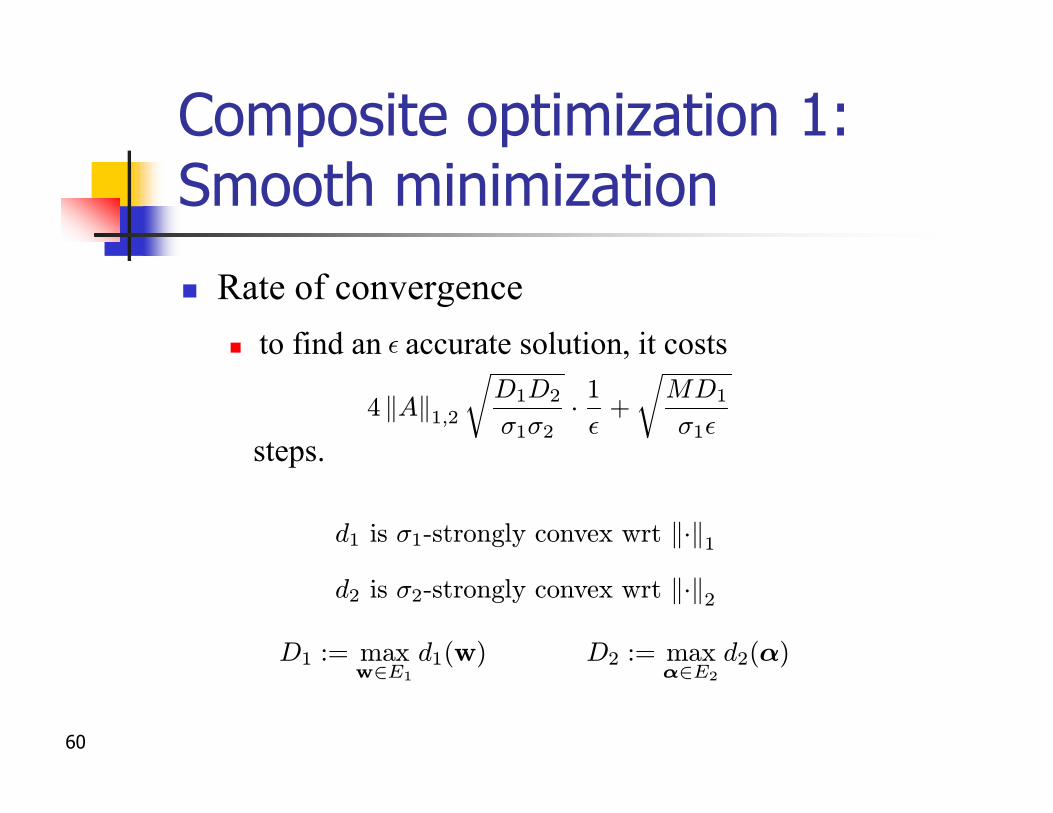
Composite optimization 1:Smooth minimization
n Rate of convergencen to find an accurate solution, it costs
steps.4 kAk1;2
rD1D2
¾1¾2¢ 1
²+
rMD1
¾1²
²
d2 is ¾2-strongly convex wrt k¢k2
d1 is ¾1-strongly convex wrt k¢k1
D1 := maxw2E1
d1(w) D2 := max®2E2
d2(®)
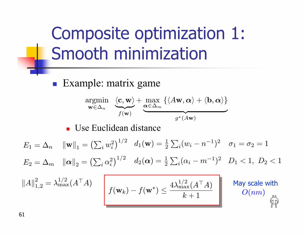
61
Composite optimization 1:Smooth minimization
n Example: matrix game
n Use Euclidean distanced1(w) = 1
2
Pi(wi ¡ n¡1)2E1 = ¢n
E2 = ¢m
argminw2¢n
hc;wi| {z }f(w)
+ max®2¢m
fhAw;®i + hb;®ig| {z }
g?(Aw)
d2(®) = 12
Pi(®i ¡m¡1)2
¾1 = ¾2 = 1
D1 < 1; D2 < 1
kAk21;2 = ¸
1=2max(A>A)
f(wk)¡ f(w¤) · 4¸1=2max(A>A)
k + 1
kwk1 =¡P
i w2i
¢1=2
May scale with
k®k2 =¡P
i ®2i
¢1=2
O(nm)
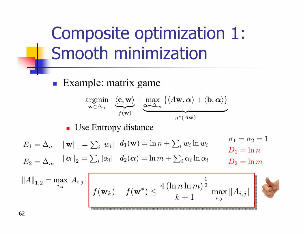
62
Composite optimization 1:Smooth minimization
n Example: matrix game
n Use Entropy distance
E1 = ¢n
E2 = ¢m
argminw2¢n
hc;wi| {z }f(w)
+ max®2¢m
fhAw;®i + hb;®ig| {z }
g?(Aw)
¾1 = ¾2 = 1kwk1 =P
i jwijk®k2 =
Pi j®ij
d1(w) = ln n +P
i wi ln wi
d2(®) = ln m +P
i ®i ln®i D2 = ln m
D1 = ln n
kAk1;2 = maxi;j
jAi;j jf(wk)¡ f(w¤) · 4 (ln n ln m)
12
k + 1maxi;j
kAi;jk
63
Composite optimization 1:Smooth minimization
n Disadvantages:n Fix the smoothing beforehand using prescribed
accuracy
n No convergence criteria because real min is unknown.
²
64
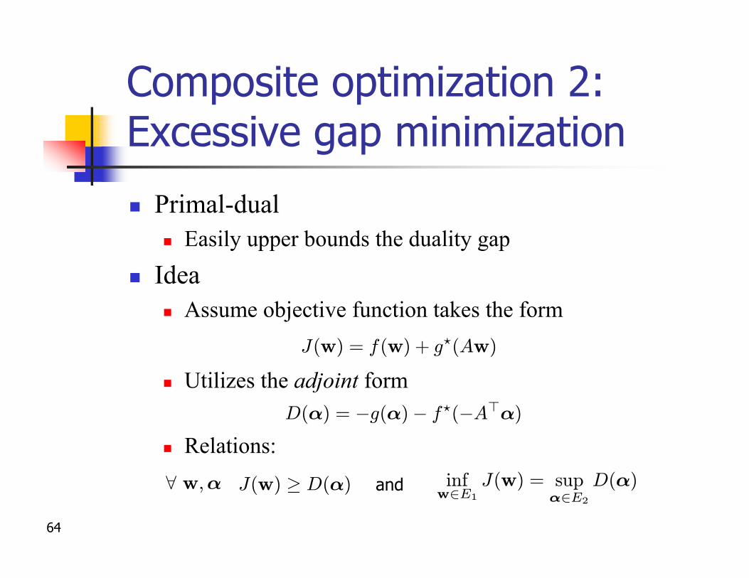
Composite optimization 2:Excessive gap minimization
n Primal-dualn Easily upper bounds the duality gap
n Idean Assume objective function takes the form
n Utilizes the adjoint form
n Relations:
J(w) = f(w) + g?(Aw)
D(®) = ¡g(®)¡ f?(¡A>®)
J(w) ¸ D(®)8 w;® and infw2E1
J(w) = sup®2E2
D(®)
65
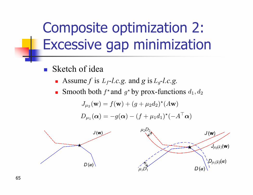
Composite optimization 2:Excessive gap minimization
n Sketch of idean Assume f is -l.c.g. and g is -l.c.g.n Smooth both and by prox-functions
J¹2(w) = f(w) + (g + ¹2d2)?(Aw)
D¹1(®) = ¡g(®)¡ (f + ¹1d1)?(¡A>®)
d1; d2
Lf Lg
f? g?
66
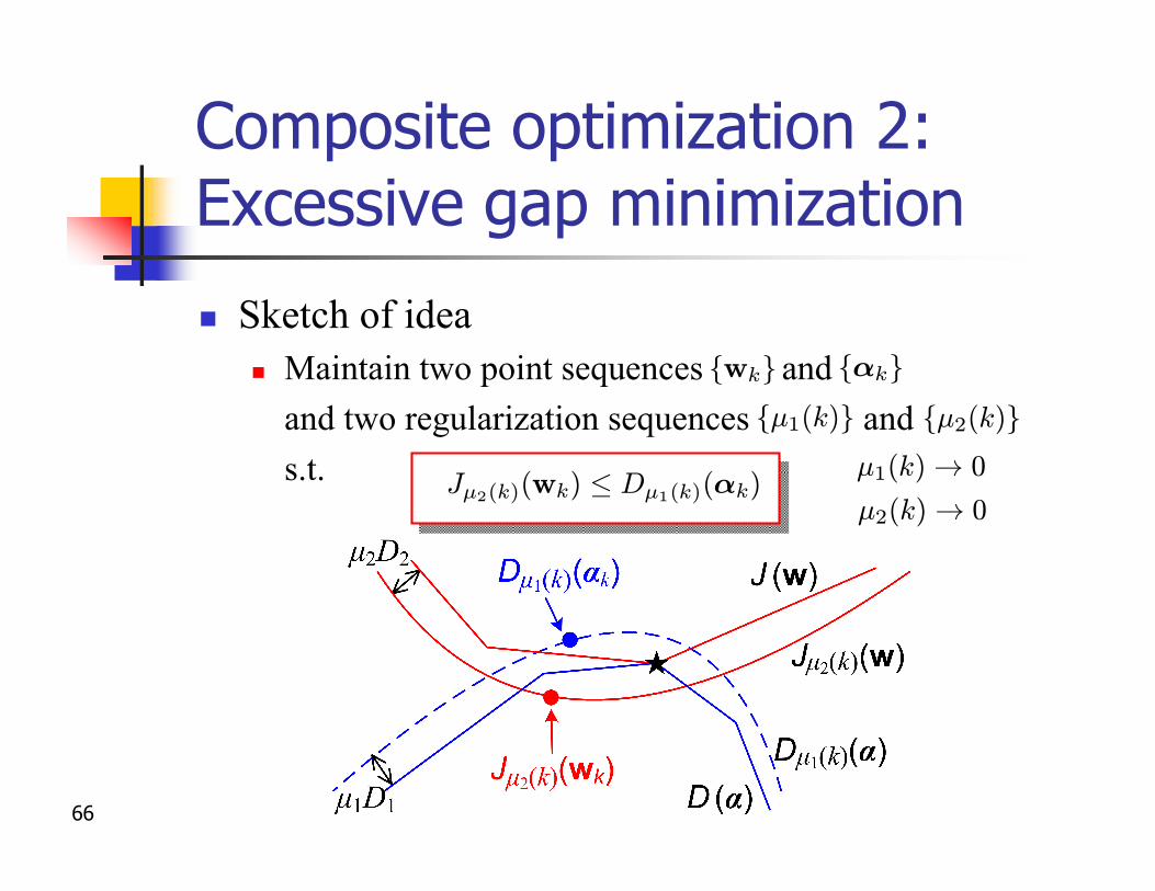
Composite optimization 2:Excessive gap minimization
n Sketch of idean Maintain two point sequences and
and two regularization sequences ands.t.
fwkg f®kgf¹1(k)g f¹2(k)g
¹1(k) ! 0
¹2(k) ! 0J¹2(k)(wk) · D¹1(k)(®k)
67
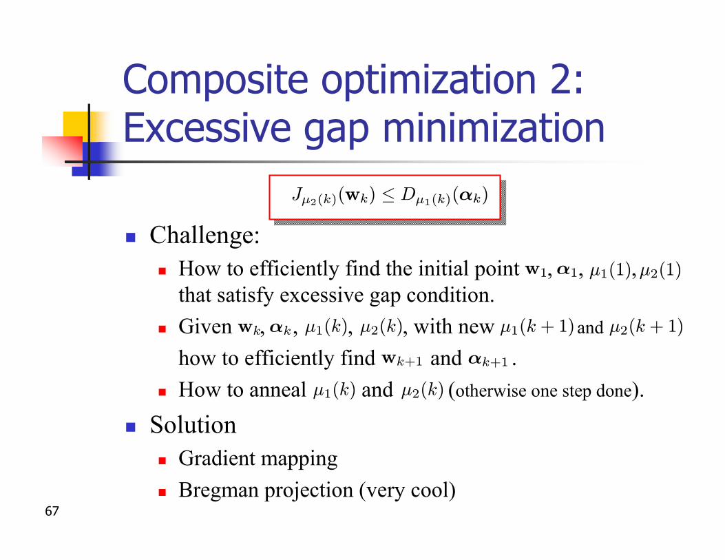
Composite optimization 2:Excessive gap minimization
n Challenge:n How to efficiently find the initial point , , ,
that satisfy excessive gap condition.n Given , , , , with new and
how to efficiently find and .n How to anneal and (otherwise one step done).
n Solutionn Gradient mappingn Bregman projection (very cool)
J¹2(k)(wk) · D¹1(k)(®k)
w1 ®1 ¹1(1) ¹2(1)
wk ®k ¹1(k) ¹2(k) ¹1(k + 1) ¹2(k + 1)
®k+1wk+1
¹1(k) ¹2(k)
68
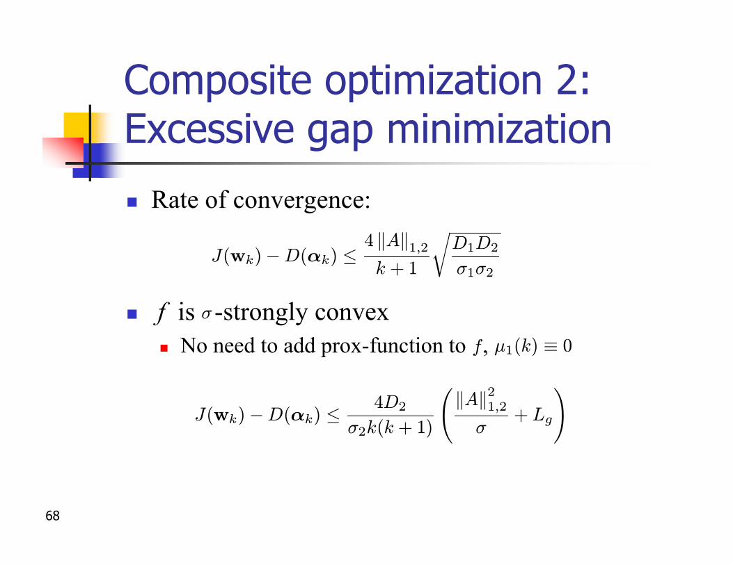
Composite optimization 2:Excessive gap minimization
n Rate of convergence:
n f is -strongly convexn No need to add prox-function to , f
J(wk)¡D(®k) ·4 kAk1;2
k + 1
rD1D2
¾1¾2
J(wk)¡D(®k) ·4D2
¾2k(k + 1)
ÃkAk2
1;2
¾+ Lg
!
¾
¹1(k) ´ 0
69
Composite optimization 2:Excessive gap minimization
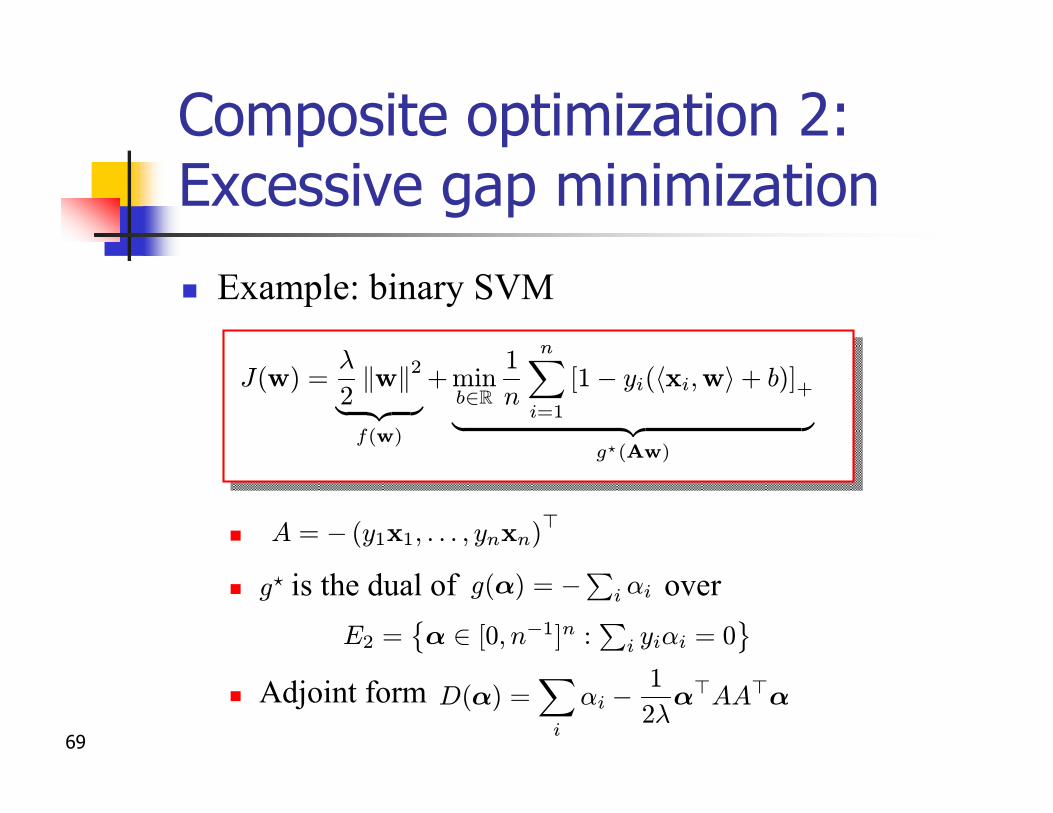
n Example: binary SVM
n
n is the dual of over
n Adjoint form
g? g(®) = ¡Pi ®i
A = ¡ (y1x1; : : : ; ynxn)>
J(w) =¸
2kwk2
| {z }f(w)
+minb2R
1
n
nX
i=1
[1¡ yi(hxi;wi + b)]+
| {z }g?(Aw)
D(®) =X
i
®i ¡1
2¸®>AA>®
E2 =©® 2 [0; n¡1]n :
Pi yi®i = 0
ª
70
Composite optimization 2:Convergence rate for SVM
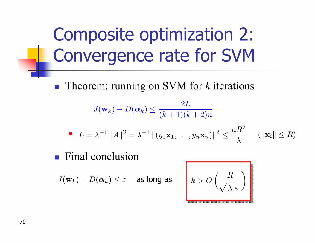
n Theorem: running on SVM for k iterations
n
n Final conclusion
J(wk)¡D(®k) · " as long as k > O
µR
11111
¶p
1="¸
(kxik · R)
J(wk)¡D(®k) ·2L
(k + 1)(k + 2)n
L = ¸¡1 kAk2= ¸¡1 k(y1x1; : : : ; ynxn)k2 · nR2
¸
71
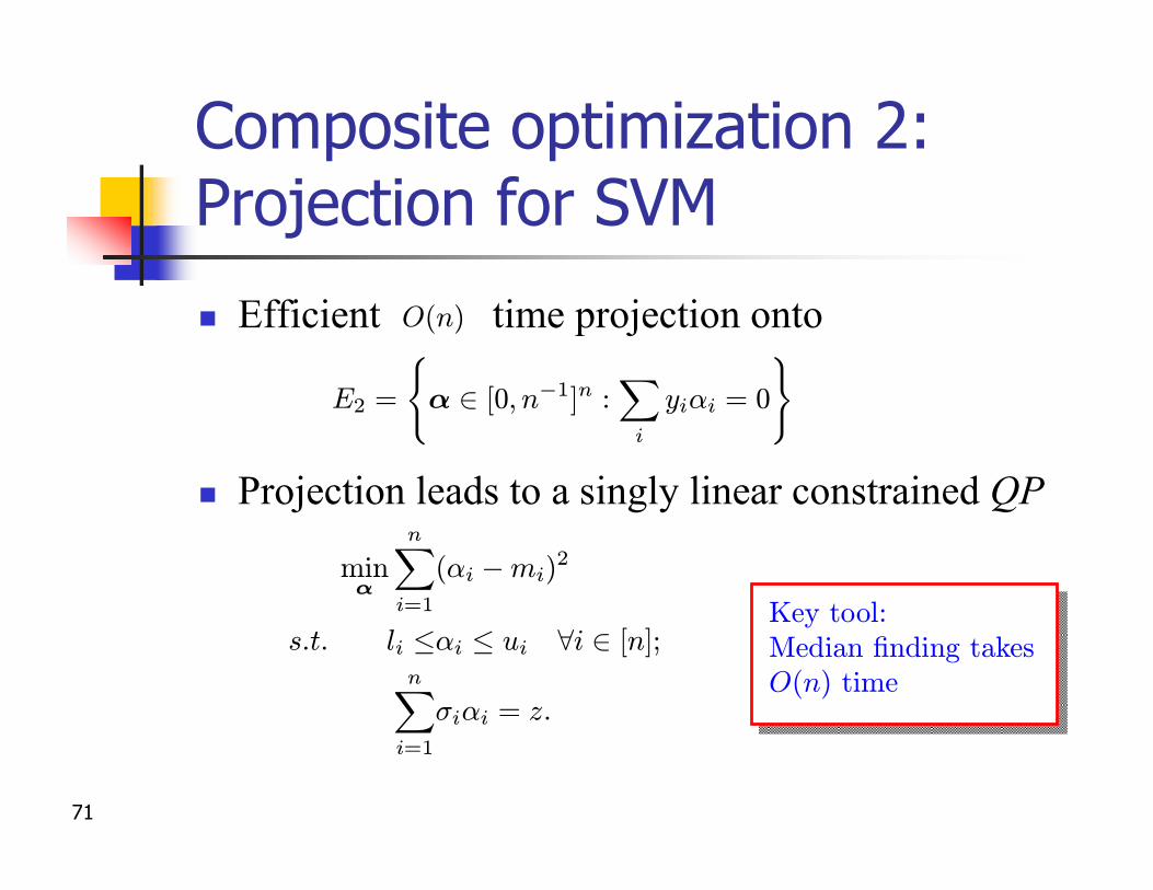
Composite optimization 2:Projection for SVM
n Efficient time projection onto
n Projection leads to a singly linear constrained QP
O(n)
min®
nX
i=1
(®i ¡mi)2
s:t: li ·®i · ui 8i 2 [n];nX
i=1
¾i®i = z:
Key tool:Median ¯nding takesO(n) time
E2 =
(® 2 [0; n¡1]n :
X
i
yi®i = 0
)
72
Automatic estimation of Lipschitz constant
n Automatic estimation of Lipschitz constantn Geometric scalingn Does not affect the rate of convergence
L
73
Conclusionn Nesterov’s method attains the lower bound
n for L-l.c.g. objectivesn Linear rate for l.c.g. and strongly convex objectives
n Composite optimizationn Attains the rate of the nice part of the function
n Handling constraintsn Gradient mapping and Bregman projectionn Essentially does not change the convergence rate
n Expecting wide applications in machine learningn Note: not in terms of generalization performance
O¡L²
¢

74