Embed Size (px)
Citation preview
18
CHAPTER-2 : PHYSICO-MATHEMATICAL
ASPECTS OF FLUID FLOW THROUGH POROUS
MEDIA
2.1 : Introduction
This chapter deals with the knowledge of very basic concepts of hydrodynamics and
basics of fluid mechanics, which is essential part of study to have better understanding
of behavior of particle in flow. This chapter deals with some useful definitions and
basic equations governing the system.
The fundamental definitions of piezometric head, piezometric slope, Filtration
(seepage) velocity, viscosity, porosity have been discussed. Also the Darcy’s law
governing the fluid flow through porous media is stated its range of validity and
general forms has been discussed.
Further the description of important phenomena like Fingering, Imbibition and
Fingero-Imbibition have been discussed.
2.2 : Fluids
A fluid is a substance which deforms continuously when subjected to shear force, no
matter how small the shear stress may be, which is perpendicular to the flow
direction.
Newton succeeded to relate shear stress with the rate of strain and this relationship is
called Newton’s law of viscosity which is given by
z � µ dudy
i.e. shear stress z is proportional to velocity gradient , and µ is viscosity co-efficient.
The fluid state refers to liquids, vapor or gaseous phases. The intermolecular attractive
forces are weaker in liquids compared to those in solids and extremely weak in vapors
and gases.
19
2.3 : Classification of Fluids
The fluids are classified on the basis of viscosity and shear stress.
(1) Ideal Fluid or Inviscid Fluid
A fluid is said to be ideal if it is assumed both inviscid and incompressible and the
resulting flow is called inviscid or ideal flow. An inviscid flow is the flow of an ideal
fluid that is assumed to have no viscosity. In an ideal flow shear force is not there
because of vanishing of viscosity.
i.e. a fluid which has no resistance to shear stress is known as an ideal fluid or
inviscid fluid.
(2) Real Fluid
All the existing fluid has got viscosity to some extent and can be compressed slightly.
In a real fluid shearing forces always develop whenever the motion takes place.
All real fluids have some resistance to stress and therefore are viscous.
(3) Viscous Fluid
In viscous fluid, both normal and shearing stress are present.
(4) Newtonian Fluid
Fluids which obey Newton’s law of viscosity i.e. z � µ ��� , is called Newtonian
fluid.
e.g. water, air, and Melton metals
Newtonian fluid is a fluid which flows like water.
(5) Non-Newtonian Fluid
A fluid, in which there is non-linear relationship of shear stress applied and resultant
angular deformation, is called non- Newtonian fluid.

20
A non-Newtonian fluid is a fluid whose flow properties differ in any way from those
of Newtonian fluids. Most commonly the viscosity (resistance to deformation or other
forces) of non-Newtonian fluids is dependent on shear rate.
e.g. plastics, Melton polymers, suspensions, paints, mud, honey , blood ,ketchup,
custard, toothpaste, starch, shampoo.
(6) Incompressible Fluids
A fluid is said to be incompressible if the density of a fluid is regarded as constant
throughout the flow field. Such assumption is possible for liquids and also for gases at
low speed. For most of the incompressible fluid, the viscosity may be regarded as
constant.
In the case of changes in pressure and temperature are sufficiently small that the
changes in density are negligible, the flow can be modeled as an incompressible flow.
(7) Compressible Fluids
A fluid is compressible and possesses no definite volume and it always expands until
its volume is equal to that of the container. Even a slight change in the temperature of
a fluid has a significant effect on its volume and pressure. All fluids are compressible
to some extent that is changes in pressure or temperature will result in changes in
density.
21
CLASSIFICATION OF FLUID ON THE BASIS OF DENSITY AND
VISCOSITY
Sr. No.
Types of Fluid
Density
Viscosity
1.
Ideal, Inviscid
Constant
Zero
2.
Real
Variable
Non-Zero
3.
Viscous
Variable
Non-Zero
4.
Newtonian
Constant or Variable
z � µdudy
5.
Non- Newtonian
Constant or Variable
z µ dudy
6.
Incompressible
Constant
Non-Zero
7.
Compressible
Variable
Zero
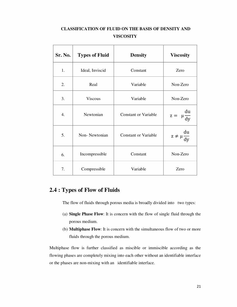
2.4 : Types of Flow of Fluids
The flow of fluids through porous media is broadly divided into two types:
(a) Single Phase Flow: It is concern with the flow of single fluid through the
porous medium.
(b) Multiphase Flow: It is concern with the simultaneous flow of two or more
fluids through the porous medium.
Multiphase flow is further classified as miscible or immiscible according as the
flowing phases are completely mixing into each other without an identifiable interface
or the phases are non-mixing with an identifiable interface.
22
In the miscible fluids flow the interfacial tension between two fluids is zero and
there is no identifiable interface between them whereas in immiscible fluid flow,
interfacial tension between the fluids is non-zero and there is a distinct (identifiable)
interface between them.
e.g. Water and ink is miscible while oil and water is immiscible flow.
The another types of flow of fluids are defined as follow:
(1) Laminar Flow: A well-ordered pattern of flow in which fluid motion occurs
in layer. i.e. one layer sliding smoothly over the adjacent layer , without
mixing with each other is called laminar flow. Any tendency towards
instability is damped out by viscous forces that also resist relative motion of
adjacent layers. Laminar flow is governed by Newton’s law of viscosity. Flow
in which turbulence is not exhibited is called laminar.
Laminar flow
• Re( Reynold number) < 2000
• low velocity
• Dye does not mix with water
• Fluid particles move in straight lines
• Simple mathematical analysis possible
• Rare in practice in water systems.
(2) Turbulent Flow: Turbulent is a state of flow in which orderly motion of fluid
particle collapses to form eddies that spread into the entire region of flow. It is
rather a state of instability of fluid motion caused by movements of adjacent
layers at different velocities. Turbulence is flow characterized by recirculation,
eddies, and apparent randomness.
The best definition of turbulent fluid motion was given by Keulegan(1938).
“Turbulent fluid motion is defined as an irregular condition of flow in which the
various quantities like density, velocity, pressure etc., show a random variation with
time and space co-ordinates, so that statistically distinct average values can be
discovered.”
23
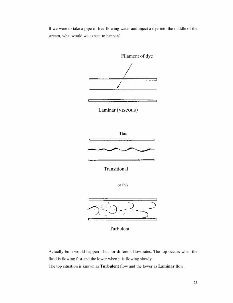
If we were to take a pipe of free flowing water and inject a dye into the middle of the
stream, what would we expect to happen?
This
or this
Actually both would happen - but for different flow rates. The top occurs when the
fluid is flowing fast and the lower when it is flowing slowly.
The top situation is known as Turbulent flow and the lower as Laminar flow.
Filament of dye
Laminar (viscous)
Transitional
Turbulent
24
Turbulent flow:
• Re > 4000
• high velocity
• Dye mixes rapidly and completely
• Particle paths completely irregular
• Average motion is in the direction of the flow
• Cannot be seen by the naked eye
• Changes/fluctuations are very difficult to detect. Must use laser.
• Mathematical analysis very difficult - so experimental measures are
used
• Most common type of flow.
Laminar flow: Re < 2000
Transitional flow: 2000 < Re < 4000
Turbulent flow: Re > 4000
Transitional flow:
• 2000 > Re < 4000
• medium. velocity
• Dye stream wavers in water - mixes slightly
(3) Steady Flow: A flow in which various hydrodynamic parameters and fluid
properties at any point do not change with time is called steady flow. When all
the time derivatives of a flow field vanish, the flow is considered to be a
steady flow. Steady-state flow refers to the condition where the fluid
properties at a point in the system do not change over time. Otherwise, flow is
called unsteady.
In Euclidean approach, velocity v� and acceleration � are functions of space
co-ordinates s only.
i.e. v�� � v�s�� and a�� � a�s��
i.e. in a steady flow , the hydrodynamics and other parameters may vary with
location.
25
Mathematically, �
�� (physical parameters of fluid) = 0
(4) Unsteady Flow : A flow in which any of the parameter changes with any of
the parameter changes with time is termed as unsteady flow.
e.g. Tidal wave
Mathematically, �
�� (physical parameters of fluid) ≠ 0
2.5 : About Porous Medium
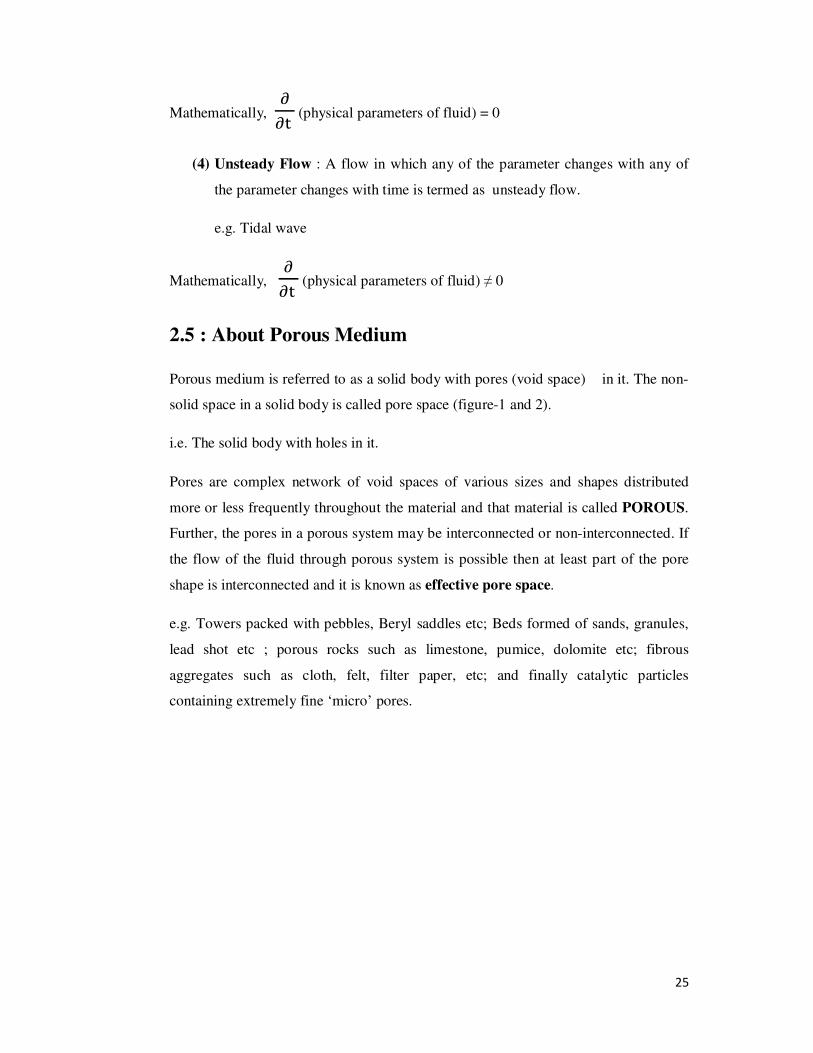
Porous medium is referred to as a solid body with pores (void space) in it. The non-
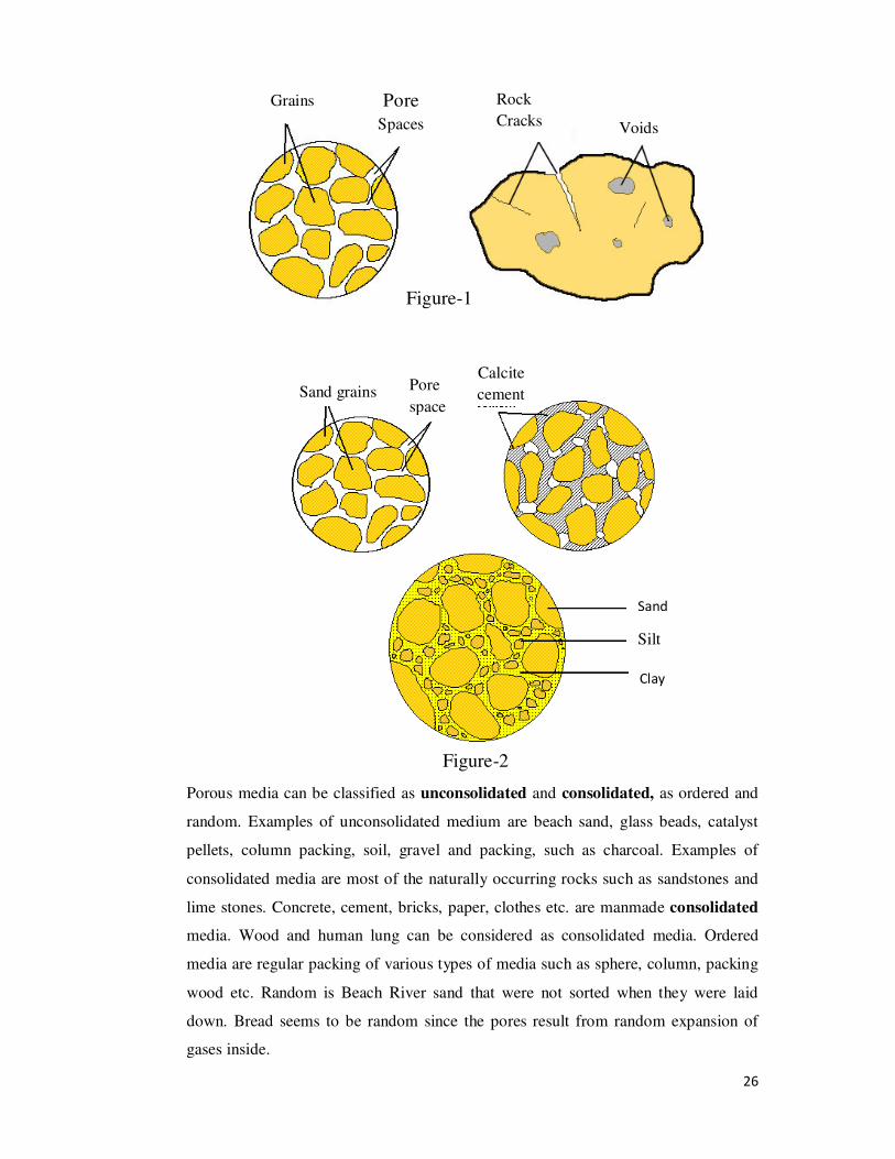
solid space in a solid body is called pore space (figure-1 and 2).
i.e. The solid body with holes in it.
Pores are complex network of void spaces of various sizes and shapes distributed
more or less frequently throughout the material and that material is called POROUS.
Further, the pores in a porous system may be interconnected or non-interconnected. If
the flow of the fluid through porous system is possible then at least part of the pore
shape is interconnected and it is known as effective pore space.
e.g. Towers packed with pebbles, Beryl saddles etc; Beds formed of sands, granules,
lead shot etc ; porous rocks such as limestone, pumice, dolomite etc; fibrous
aggregates such as cloth, felt, filter paper, etc; and finally catalytic particles
containing extremely fine ‘micro’ pores.
26
Porous media can be classified as unconsolidated and consolidated, as ordered and
random. Examples of unconsolidated medium are beach sand, glass beads, catalyst
pellets, column packing, soil, gravel and packing, such as charcoal. Examples of
consolidated media are most of the naturally occurring rocks such as sandstones and
lime stones. Concrete, cement, bricks, paper, clothes etc. are manmade consolidated
media. Wood and human lung can be considered as consolidated media. Ordered
media are regular packing of various types of media such as sphere, column, packing
wood etc. Random is Beach River sand that were not sorted when they were laid
down. Bread seems to be random since the pores result from random expansion of
gases inside.
Figure-1
Figure-2
Grains Pore
Spaces
Rock
Cracks Voids
Figure-1
Sand grains Pore
space
Calcite
cement
Sand
Silt
Clay
27
Moreover, pores occupy the fraction of volume of the bulk volume of the porous
medium by making a complex network of interconnected openings and which is
responsible for the flow of contained fluid. The porous medium may be homogeneous
or heterogeneous depending upon whether its characteristics are uniform throughout
or variable.
2.6 : Geometrical Properties of Porous Medium
For any porous material to form a reservoir:
(a) It must have a certain storage capacity; this property is characterized by the
porosity.
(b) The fluids must be able to flow in the medium; this is characterized by
permeability.
(c) It must contain a sufficient quantity of fluids with a sufficient concentration;
the impregnated volume is a factor here, as well as the saturation.
Porous medium is characterized by various geometrical properties but for the purpose
of mathematical modeling of the flow through them, we consider only porosity,
permeability and tortuosity.
2.6.1 : Porosity
Porous medium must have a certain storage capacity; this property is characterized by
porosity. Porosity is an index how much fluids can be stored within the medium.
The average porosity or simply porosity of a sample of a porous medium is defined as
the ratio of interconnected pore volume VP to the total volume (or bulk volume) VT
of a sample. The volume VT includes solid as well as pore volume. It is defined by φ .
i.e. φ � ������ �� �����T�� � ������ � VP
VT
It Is expressed as the percentage of the total volume of the porous medium.
φ (in percentage) = 100 $1 & VGVT(
Where VG is the grain volume of a sample. Obviously φ is a dimensionless quantity.
28
Porosity at a point is an abstraction that cannot be measured experimentally. Only the
average porosity of a material can be measured.
From the inherent nature of consolidated porous material, it is apparent that, while
their voids pores will in general be interconnected, some may become sealed off
during the course of cementation of the material.
Effective porosity φE corresponds to the pores connected to each other and to the
formations.
Effective Porosity φE = E���-�.�� ���� �� -�
T�� � ������
Total porosity φT is also defined as, corresponding to all the pores whether
interconnected or not, and the residual φ� , which only takes account of isolated
pores.
φT= φE + φ�
The effective porosity of rocks varies between less than 1% and over 40%. For
fractured rock, the fractured porosity related to the rock volume is often much less
than 1%.
Effective porosity is of practical interest with respect to oil-production and, therefore,
it is common practice to use term porosity for that of effective porosity. Numbers of
investigation have been made an attempt to determine the porosity [53-55] and it was
found that it vary from 0.04 to 0.93 depending on the porous materials [56].
Thus porosity is an important physical characteristic of the porous media which
determines the quantity of oil and water present in problems of petroleum recovery or
in general, the volume of flowing phase in the medium. There are several methods
available to determine porosity [57].
2.6.2 : Permeability
Permeability is a measure of an ease with which fluids pass- through a porous
material. The specific or absolute permeability of a porous medium is the ability of
the medium to allow a fluid with which it is saturated to flow through its pores. It is
29
measured by the rate of flow. In such a case the medium is said to be permeable or
pervious. On the other hand, those through which fluid cannot easily soak are called
impermeable or impervious medium. e.g. they may be of two kinds . Porous like clay
and non-porous like massive unfisssured granite.
It is closely related to the size of the voids and the degree to which they are
interconnected. If the voids are small and scarcely interconnected, the medium will
transmit fluids very slowly. If they are large and interconnected, the medium will
transmit the fluids very freely.
The permeability depends on the property of the medium and is independent of the
fluid properties.
The units for determining permeability are gallons/ day/ft, cm1, ft1, Darcy, m/s and
f/s used by many organizations and disciplines.
The common expressions for permeability k is ;
k � & QµAρg :∂h
∂s=>?
Where Q is the volume of fluid discharged per unit time
A is the cross- sectional area
µ is the viscosity
ρ is the fluid density
�@�ρ is the hydraulic gradient in the direction of flow
k has the dimensions of L2 . The unit L is named after French hydraulic engineer
“ Henry Darcy” and is defined as “The permeability of porous medium is 1 Darcy if
through it will flow 1 centimeter per second of a fluid of 1 centipoises viscosity under
the action of 1 ��-� pressure gradient” [59].

30
The absolute permeability, defined above, depends on the direction considered. In
particular, the horizontal permeability kh (parallel flow towards the medium) and
vertical permeability kv (serration problems of fluids of different densities) are
defined. Due to stratification, the kv is generally much lower than kh.
2.6.3 : Porosity / Permeability Relationship
The correlation between porosity and permeability for a given material is given by
log k � aφ D b, where � and b are constants.
2.6.4 : Tortuosity
It is the relative average length of the flow path of a fluid particle from one side of the
porous medium to the other. It is a dimensionless quantity. It is denoted by τ.
2.7 : Phase Composition
When various fluid phases occupy a certain fraction of the bulk volume, there are
several ways commonly used to describe the amount of each fluid contained in the
medium. That fraction for j is known as the phase content θF. The fraction of the void
space occupied by phase j is known as the phase (degree of) saturation, sj . The mass
fraction of a solute a per volume of solution is known as the concentration HI .
In the pore volume VP are found a sum of volume Vw of water , a volume Vo of oil
and a volume VG of gas , i.e. Vw + Vo+ VG= VP
The oil, water and gas saturations are:
So = VJVP , SW =
VWVP and SG =
VGVP expressed in percent, with
So +SW+ SG = 100 %
Displacement of one fluid by another is called desaturation. The term ‘saturated”
means that only a one phase j exists throughout the medium and in such case Sj is 1.0
In petroleum literature the term residual or irreducible saturation (Sr) is used, which is
31
the value of saturation at which Pc (capillary pressure defined later) increases very
rapidly with negligible decrease in saturation. The immobilizes drops are called
“residual fluid”.
Because the pore space containing the wetting phase at Swet Q Sr contributes
relatively very little to connective flow process, it is convenient to define an effective
saturation Se given by
Se � �RSTUVW?> �W The relationship among the three expressions for phase content is
θF = φSj , where X is the porosity of the medium.
2.8 : Capillary Mechanism
2.8.1 : Wettability
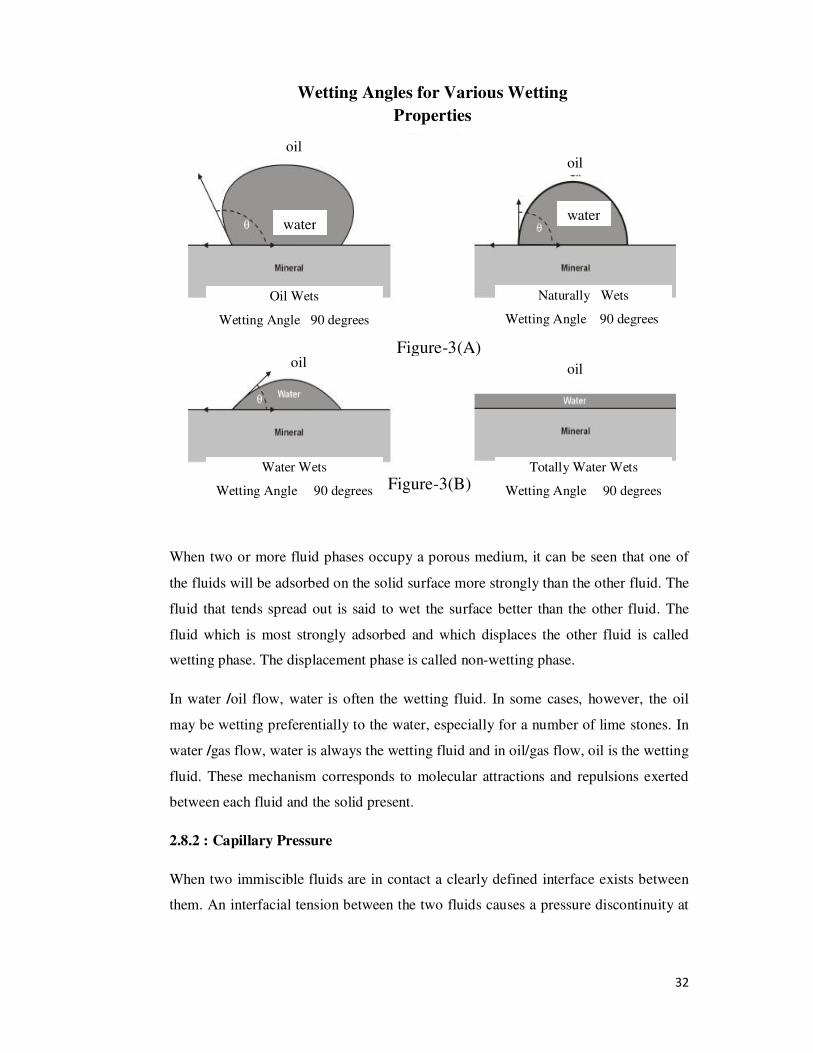
When two immiscible fluids, such as oil and water, are together in contact with a rock
face the situation is as depicted in [Figure-3(A) and Figure-3(B)]. The angle θ,
measured through the water is called the contact angle. If θ < 900 reservoir rock is
described as being water wet, whereas if θ > 900 it is oil wet. The wet ability, as
defined as the angle, is a measure of which fluid preferentially adheres to the rock.
32
When two or more fluid phases occupy a porous medium, it can be seen that one of
the fluids will be adsorbed on the solid surface more strongly than the other fluid. The
fluid that tends spread out is said to wet the surface better than the other fluid. The
fluid which is most strongly adsorbed and which displaces the other fluid is called
wetting phase. The displacement phase is called non-wetting phase.
In water /oil flow, water is often the wetting fluid. In some cases, however, the oil
may be wetting preferentially to the water, especially for a number of lime stones. In
water /gas flow, water is always the wetting fluid and in oil/gas flow, oil is the wetting
fluid. These mechanism corresponds to molecular attractions and repulsions exerted
between each fluid and the solid present.
2.8.2 : Capillary Pressure
When two immiscible fluids are in contact a clearly defined interface exists between
them. An interfacial tension between the two fluids causes a pressure discontinuity at
Figure-3(A)
oil
water
oil
water
Figure-3(B)
Oil Wets
Wetting Angle 90 degrees
Water Wets
Wetting Angle 90 degrees
Naturally Wets
Wetting Angle 90 degrees
Totally Water Wets
Wetting Angle 90 degrees
Wetting Angles for Various Wetting
Properties
oil oil
33
the boundary separating the two fluids and this pressure is known as capillary
pressure. It is denoted by P- and is defined by
PC � PZ & P.
Where PZ and P. are the pressure of native and injected phases respectively.
The difference in pressures between phases occupying the pore space of a porous
medium is related to gravity, saturation , pore size, pore shape , interfacial forces, the
angle at which fluid interface contact solid-solid interface, the density difference
between phases and the radii of curvature of interfaces. These factors are not all
independent variables in respect to their effect on PC .There is, however, an inter
relation among them.
It is an equilibrium property, directly related to interfacial tension, [Morrow, 1970].
The equilibrium condition is expressed by Laplace equation
PC � σ : 1r? D 1
r1=
Where [ is the interfacial tension between two fluids and r? and \1 are two principal
radii of curvature of the interface at any point.
The changes in interfacial curvatures and Pc are accompanied by a change in fluid
saturation.
Pc(s) is the most important functional relationship in respect to the mechanics of
mixed fluids in porous media close together and situated on either side of the
interface:
Pc = Pnw + Pw
Pnw and Pw being the pressure of the non-wetting and wetting phases respectively.
The forgoing discussion shows that, for a medium saturated with a fluid and
surrounded by another fluid:
34
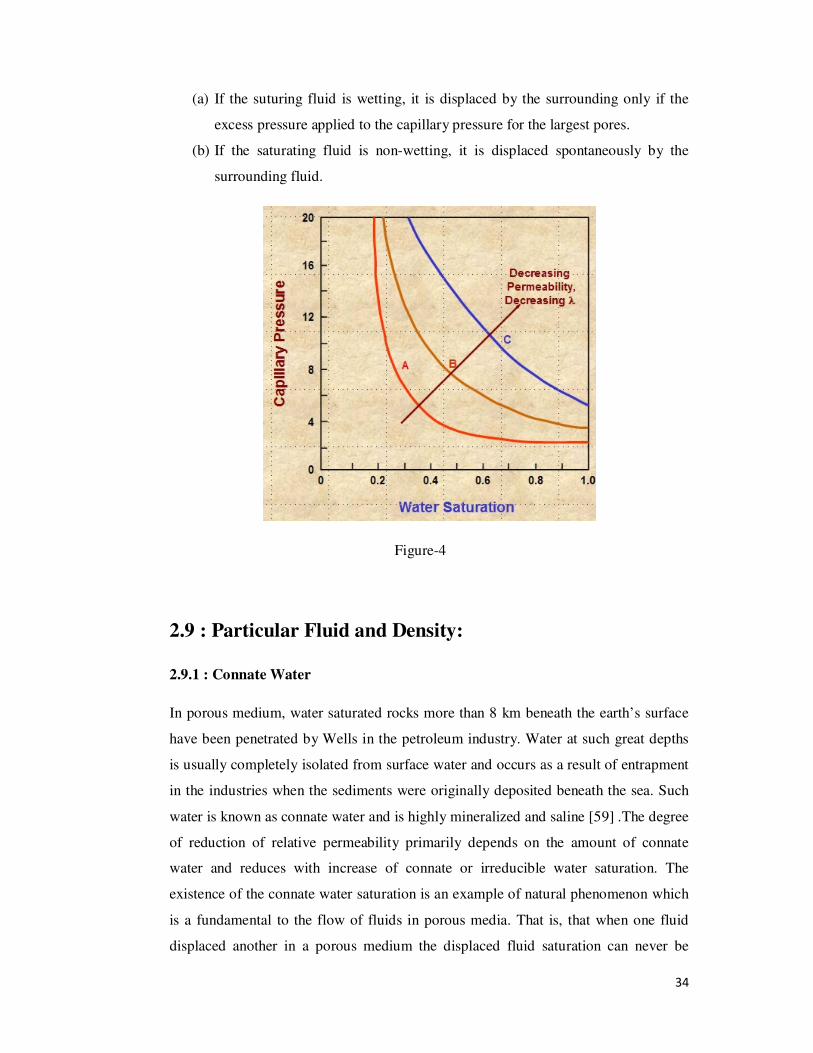
(a) If the suturing fluid is wetting, it is displaced by the surrounding only if the
excess pressure applied to the capillary pressure for the largest pores.
(b) If the saturating fluid is non-wetting, it is displaced spontaneously by the
surrounding fluid.
Figure-4
2.9 : Particular Fluid and Density:
2.9.1 : Connate Water
In porous medium, water saturated rocks more than 8 km beneath the earth’s surface
have been penetrated by Wells in the petroleum industry. Water at such great depths
is usually completely isolated from surface water and occurs as a result of entrapment
in the industries when the sediments were originally deposited beneath the sea. Such
water is known as connate water and is highly mineralized and saline [59] .The degree
of reduction of relative permeability primarily depends on the amount of connate
water and reduces with increase of connate or irreducible water saturation. The
existence of the connate water saturation is an example of natural phenomenon which
is a fundamental to the flow of fluids in porous media. That is, that when one fluid
displaced another in a porous medium the displaced fluid saturation can never be
35
reduced to zero. It was known that connate water saturation varies over a wide range
of 10 to 80 % and depends on the petro physical characteristics of rock.
2.9.2 :Fluid Density
Fluid density is defined as the mass per unit volume is generally varies with pressure
and temperature according to the relation called equation of stated (any equation
which relate p (pressure), ](density) and T(temperature).
In other words,
ρ = ρ(P,T) or f( ρ, P,T) = 0
Dimensional formula for “density” is ML-3 in physical system (MLT) and FT-2L-4 in
technical (FLT) system.
While dealing with the role of groundwater in a production mechanism,
compressibility of the water must be taken into consideration [60].
Muskat [61] has given the following general equation (including all fluids of practical
significance and all thermodynamic types of various flows) for the variation in the
fluid density.
ρ = ρE + _ a ebPcccc
Where P is the fluid pressure, ρE is some definite constant, and ma and kc are constant
parameters.
The classification for particular, fluids of physical significance is as follow:
Liquid : ma = 0
Incompressible liquids: kc = 0
Compressible liquids: kc 0
Gases: kc = 0
Isothermal expansion: ma = 1

36
Adiabatic expansion = ���-.f.- @� � � -�Z�� Z� ������ ���-.f.- @� � � -�Z� Z� ��������
2.10 : Basic Definitions
2.10.1 : Viscosity
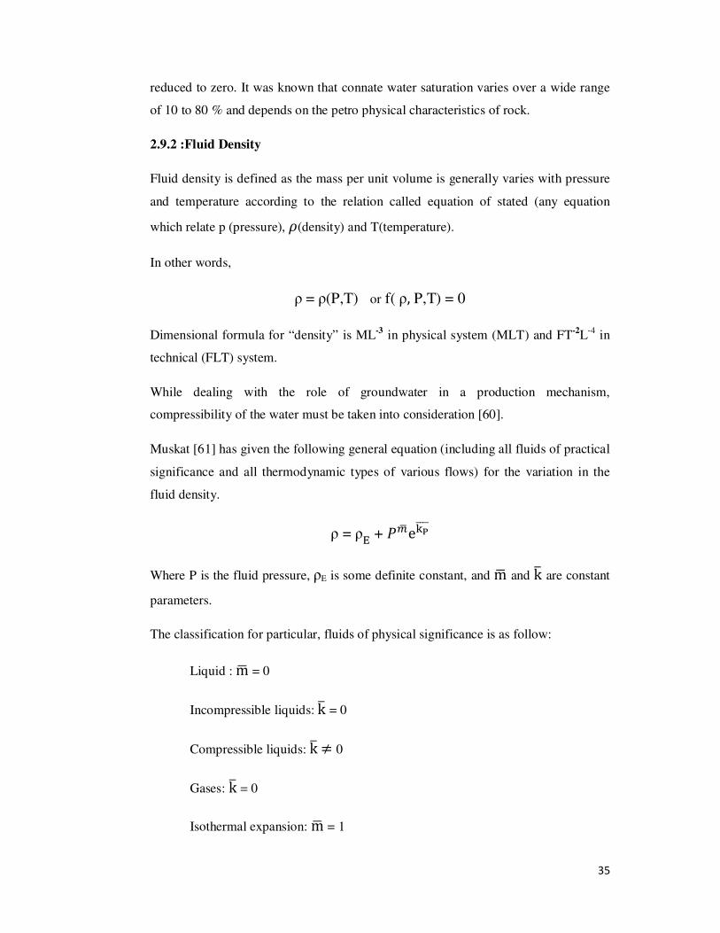
Viscosity is measure of the resistance offered to movements between two adjacent
layers of fluids. Throughout this work it is assumed to be constant. Viscosity of a
fluid varies with pressure and temperature. Temperature being constant, viscosity
rises with rise in pressure, and at constant pressure viscosity increases with decrease
in temperature.
In everyday terms (and for fluids only), viscosity is “thickness’’ or “internal friction”.
Thus water is “thin”, having a lower viscosity, while honey is “thick”, having a higher
viscosity.
Temperature plays the main role in determining viscosity.
Temperature
[°C]
Viscosity
[mPa•s]
10 1.308
20 1.002
30 0.7978
40 0.6531
50 0.5471
60 0.4668
70 0.4044
80 0.355
90 0.315
100 0.282
37
2.10.2 : Piezometric Head and Slope
The steady state Bernoulli’s equation from hydraulics for an incompressible and
inviscid fluid in a pipe (horizontal on inclined) with smooth walls is given by,
Where P is water pressure (N/M2)
is water density (kg/M3)
g is acceleration due to gravity (m/s2)
v is velocity (m/s)
z is elevation or geometric height above a certain datum
plane (m)
r is water specific weight
Liquid water
Critical
point
Super-
critical
water
Experimental Data Points from Dortmund Data
Dynamic Viscosity Water
Temperature [k]
38
Here Pρf is called piezometric height and
�g1f is velocity head at any point within the
region of the flow.
The piezometric head or hydraulic head h at a specific point is the sum of the
pressure head and the elevation.
h � Pρf D z ----------------------------- (2.10.1)
h � P� D z ------------------------------ (2.10.2)
Equation (2.10.1) is the normal ST form while second is the usual form used with the
English units.
Piezometric Slope
The piezometric slope (J) or gradient of the piezometric head is defined as the
deviation h along the path of flow.
i.e. J � & �@�� � & lim∆�kl m@
m� -----------------------(2.10.3)
Where h is the head drop and s is the distance. The negative sign indicates the flow in
the direction of describing head h.
2.10.3 : Seepage or Filtration Velocity
The seepage (Filtration velocity) can be defined as the flux of fluid (volume of fluid)
flowing per unit time across a unit area of the porous medium through which it is
flowing.
An elementary area of porous media in the soil composed of sections of soil grains
and gaps between these sections. On account of the complicated nature of the flow of
fluid between the grains of soil, it has been adopted not to consider the true velocity
of the fluid at different points but average value of these velocities. This microscopic
velocity of fluid through the porous media is called seepage (filtration) velocity.
2.10.4 : Reynolds Number For The Fluid

39
Reynolds number is named after Osborne Reynolds (1842-1912), who proposed it in
1883. Reynolds number is a dimensionless quantity associated with the smoothness of
flow of fluid. It is the most important quantity used in aerodynamics and
hydrodynamics.
At low velocities fluid can be pictured as a series of parallel layers or laminar, moving
in different velocities. Laminar flow occurs at low Reynolds’ number, where viscous
forces are dominant, and is characterized by smooth, constant fluid motion.
As the fluid flows more rapidly the motion changes from laminar to turbulent.
Turbulent flow occurs at high Reynolds number and is dominated by inertial forces,
producing random eddies, vertices and other flow fluctuations.
Reynolds number is used for determining whether a flow will be laminar or
turbulent.Reynolds number is the ratio of inertial forces (Uρ) to viscous forces$µL(,
is denoted as Re
op = IZ���. � F��-��V.�-��� F��-��
= UρLµ
= ULV
Where U is characteristic velocity
L is characteristic length
ρ is mass density
µ is viscosity
v is kinetic viscosity
2.10.5 : Bulk Density
40
Bulk density of solid is defined as the ratio of mass of soil over the bulk volume of
soil crossing of soil and gas phases.
Bulk density of fine textured surface soils are commonly in the range of 1.1 to 1.3
gm.cm-3
, and that of course texture soil are in the range of 1.4 to 1.8 gm.cm-3
Soil Bulk Density =
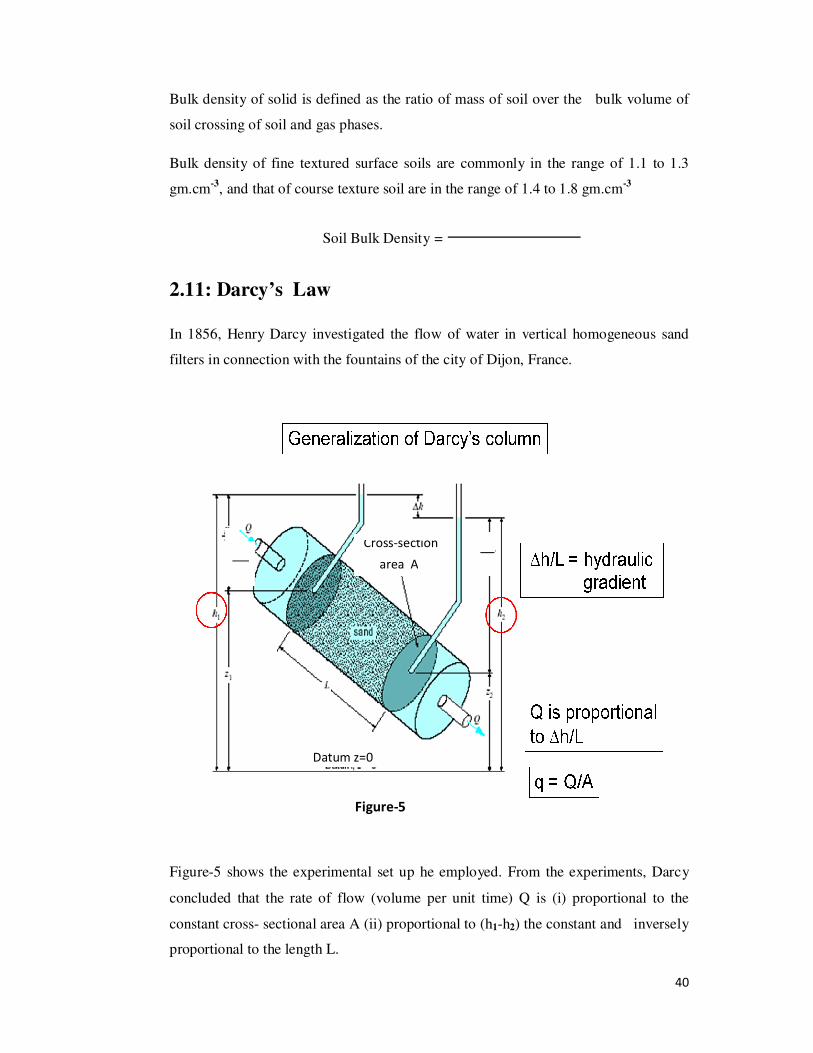
2.11: Darcy’s Law
In 1856, Henry Darcy investigated the flow of water in vertical homogeneous sand
filters in connection with the fountains of the city of Dijon, France.
Figure-5 shows the experimental set up he employed. From the experiments, Darcy
concluded that the rate of flow (volume per unit time) Q is (i) proportional to the
constant cross- sectional area A (ii) proportional to (h1-h2) the constant and inversely
proportional to the length L.
Figure-5
Datum z=0
Q Cross-section
area A
41
Q � KA��@v>@g �L . =
KA��@v>@g �∆� -------------(2.11.1)
Where K is a constant of proportionality. The length h1 and h2 are measured with
respect to some arbitrary (horizontal) datum level.
Denoting �wv>wg �x = y (hydraulic gradient) and defining the specific discharge q
as discharge per unit cross sectional area normal to the direction of flow z � I{
| q � KJ --------------------------- (2.11.2)
(2.11.2) is another form of Darcy’s formula.
Darcy’s law can be extended to flow through an inclined homogenous porous medium
column.
� � KA�φv>φg �L .
| q � K�φv>φg �L � KJ ---------------------- (2.11.3)
Where X� � � D ��� , ∆X � �X? & X1 �
The energy loss is due to friction in the flow through the narrow tortuous paths of the
porous medium. Actually the total mechanical energy of the fluid includes a kinetic
energy.
However, changes in the piezometric head are larger than changes in the kinetic
energy head along the flow path; the kinetic energy is neglected when considering the
head loss along the flow.
From this form of Darcy’s law, it is important to note that the flow takes place from a
higher piezometric head to a lower pressure.
p?r Q p1r
42
(i.e. the flow is in direction of increasing pressure and decreasing piezometric head )
φ � z D pr
Experimentally derived form of Darcy’s law (for a homogeneous incompressible
fluid) was limited to one dimensional flow.
When the flow is three dimensional then Darcy’s law is given by
q � KJ � &K gradφ
Where z is the specific flux vector with components z� , z� , z� in the directions of
the Cartesian co-ordinates � , �, � respectively. And J � &gradφ , is the hydraulic
gradient with components y� � & ���� , y� � & ��
�� , y� � & ���� in the � , �, �
respectively.
This equation remain valid for three dimensional flow through homogeneous
isotropic media, where � � ���, �, ��.
General Form of Darcy’s Law
For a three dimensional flow system, the obvious generalization is that the
resultant velocity at any point is directly proportional to, in magnitude and direction,
to the resultant hydraulic gradient at that point. The generalized form of Darcy’s law
may be written as
� � &� �\���
� &� �\��X , where X � �� ------------------- (2.11.4)
Where X is the velocity potential. Interestingly, this implies that the flow in
homogeneous porous media is irrotational. This statement reflects only the
microscopic flow behavior when it may be explained that the rotations within the
interstices balance out statistically.
The alternative form of the equation (2.11.4) in terms of pressure is
43
� ��� � & �� ��\��� & ]��\���� ---------------------- (2.11.5)
Where � ��� is the volume flux (per unit area)
ρ is mass density
µ is viscosity
P is pressure
� is acceleration due to gravity.
For a three dimensional Cartesian co-ordinate system equation (2.11.5) can be
written as
�� � & ���
����
�� � & ���
����
�� � & ��� $��
�� & ]�(
Where the z-axis is directed downwards and the possibly different
permeability in different directions is so designated.
2.12: Additional Mathematical Concepts Required For The
Multiphase Fluid Flow
Numerous quantitative investigations [2] have proved that the immiscible fluid flow
through porous media may be desired by Darcy’s equation provided if it is applied to
each phase individually and the associated permabilities are considered as a function
of phase saturation only. This extension of Darcy’s law to the flow of double phase
immiscible of fluid has been suggested by MUSKAT[61] and confirmed by a number
of subsequent researchers. The pressure of the individual phases is also to be
expressed separately since they change discontinuity across the curved interface
between the following phases. These concepts give rise to new definitions as below:
44
2.12.1 : Relative Permeability
For the single phase flow through porous media, the permeability refers to the flow
capacity of the rock or porous medium and which is independent of the nature fluid
provided the fluid occupies the whole of the void space and depends only on the
characteristics of the medium and it is termed as total or absolute permeability. Thus
an absolute total permeability when the rock is completely filled or saturated with a
single phase.
The ability of two fluids to flow simultaneously through porous medium depends not
only on the permeability but also on the relative amounts of the fluids filling the pore
spaces. Thus, the above concept is modified by introducing effective and relative
permeability.
It is natural that, when a two or more phases are flowing in a porous media, the part of
the space will be occupied by each phases and so the resistance of flow of single
phase would increase. i.e. permeability to this fluid would be less if it alone filled the
whole pore space of the medium. In complicated structure of the medium and its
fluids, the flow capacities must be expressed in terms of permeabilities to separate
phases present. The absolute magnitudes of these flow capacities are called effective
permeabilities.
In multiphase fluid flow, at least two fluids are always present in the medium. Darcy’s
law serves to determine an effective permeability for each of the fields. Since the
pressures in two fluids differ due to capillary mechanism, the concept of relative
permeability is mainly employed.
The effective permeability of a fluid is defined as the permeability when porous
medium is only partly filled with the fluid. Effective permeability is point function of
saturation. The relative permeability is defined as follow:
Relative permeability = E���-�.�� ����� �.�.� �� �.������ �.�.� �� �@� ���.��
i.e. k�� � b�b
45
These relative permeabilities depend on the medium concerned and the proportions of
the fluids present.
If two fluids flow simultaneously in medium, this can be observed to reduce the
permeability of each fluid. Effective permeability depends on the specific
permeability of the medium and on the saturations. If we consider a sample saturated
with oil and slowly inject water the permeability to oil decreases stead. It is not
substantially affected by the pressure of oil. Also k�� D k�R Q 1, which shows that
both fluids mutually hinder each other during their simultaneous movements, means
the total flow capacity is reduced. The concept of relative permeability is intended to
extend the concept of permeability to two- phase flow in a simple way. Thus Darcy’s
law can be used directly.
The effective porosity, maximum pore size, pore size distribution, effective saturation
are the affecting factors to the relative permeability.
It has been proved by number of investigations that the relative permeabilities to
immiscible fluids are within reasonable limits, functions of saturation only. The
method of relative permeability measurement can be divided in to two classes- those
are used in steady state flow conditions and those that are used in unsteady state
displacement of one fluid by another. The most rapid of the methods of measuring
relative permeability are unsteady state method such as the gas drive water drive
methods.
Summarizing, the relative permeability saturation relations are independent of flow-
rate, fluid viscosities and interfacial tension. By interface they are also independent of
the pressure level and the temperature, while relative permeability are dependent on
saturation and on the rock characteristic such as the pore size and the wet ability. A
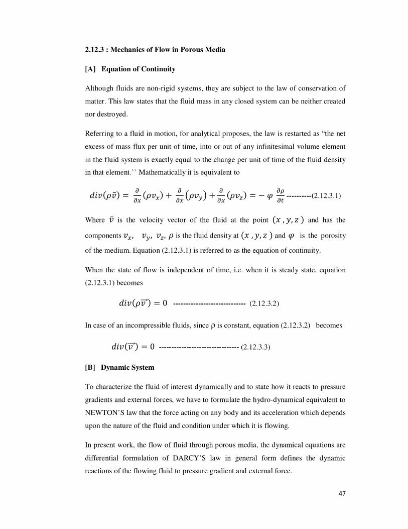
typical physical relative permeability curve and dependence on phase saturation is
shown in the following figure-6.
46
2.12.2 : Phase Saturation
The void space of a porous material may be partially filled with a liquid and the
remaining void space being occupied by air or gas or two immiscible liquids jointly
fill the void space. In either of these cases the fluids jointly filling the void space, the
question is how much of the void space is occupied by each fluid is very important.
The saturation of porous medium with respect to a particular fluid is defined as
follow:
Where is the saturation with respect to fluid w.
Thus for two fluids viz; oil and water say jointly filling the void space, it follows that
+ = 1
We observed that saturation to bulk properly which ignores the relative distributions
of the fluids within the porous structure of the porous material. We also note that
saturation is a dimensionless quantity.
Fig-6:Typical oil & water permeability curves
Water Saturation: Percent Pore Space
47
2.12.3 : Mechanics of Flow in Porous Media
[A] Equation of Continuity
Although fluids are non-rigid systems, they are subject to the law of conservation of
matter. This law states that the fluid mass in any closed system can be neither created
nor destroyed.
Referring to a fluid in motion, for analytical proposes, the law is restarted as “the net
excess of mass flux per unit of time, into or out of any infinitesimal volume element
in the fluid system is exactly equal to the change per unit of time of the fluid density
in that element.’’ Mathematically it is equivalent to
����]��� � ��� �]��� D �
�� �]��� D ��� �]��� � & X ��
� ----------(2.12.3.1)
Where �� is the velocity vector of the fluid at the point �� , �, � � and has the
components ��, ��, ��, ] is the fluid density at �� , �, � � and X is the porosity
of the medium. Equation (2.12.3.1) is referred to as the equation of continuity.
When the state of flow is independent of time, i.e. when it is steady state, equation
(2.12.3.1) becomes
����]� ��� � � 0 ----------------------------- (2.12.3.2)
In case of an incompressible fluids, since ρ is constant, equation (2.12.3.2) becomes
����� ��� � � 0 -------------------------------- (2.12.3.3)
[B] Dynamic System
To characterize the fluid of interest dynamically and to state how it reacts to pressure
gradients and external forces, we have to formulate the hydro-dynamical equivalent to
NEWTON’S law that the force acting on any body and its acceleration which depends
upon the nature of the fluid and condition under which it is flowing.
In present work, the flow of fluid through porous media, the dynamical equations are
differential formulation of DARCY’S law in general form defines the dynamic
reactions of the flowing fluid to pressure gradient and external force.
48
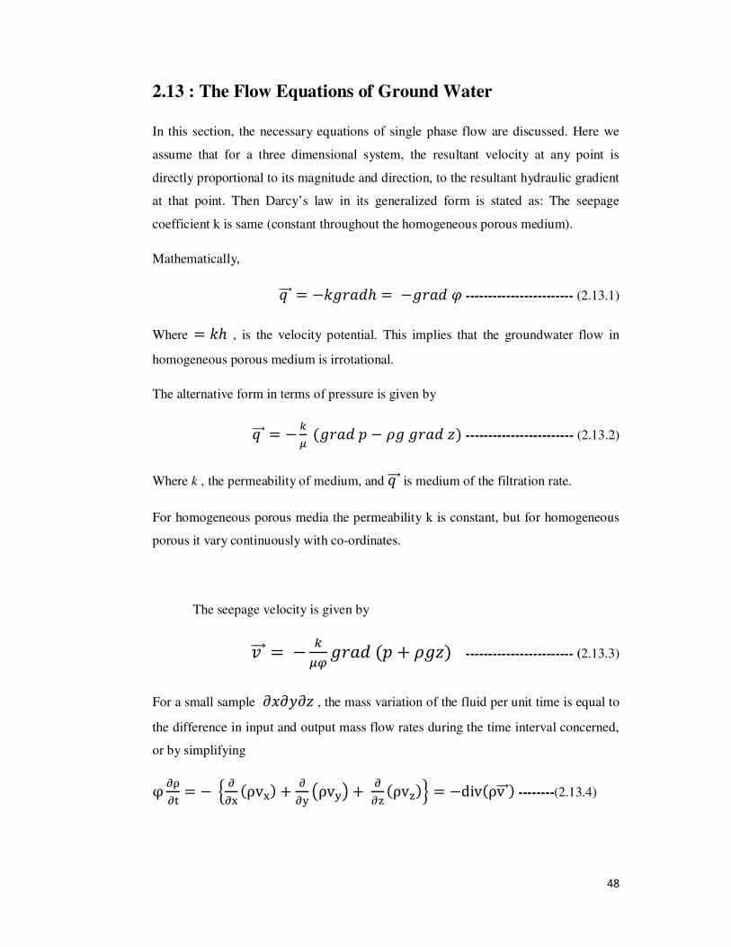
2.13 : The Flow Equations of Ground Water
In this section, the necessary equations of single phase flow are discussed. Here we
assume that for a three dimensional system, the resultant velocity at any point is
directly proportional to its magnitude and direction, to the resultant hydraulic gradient
at that point. Then Darcy’s law in its generalized form is stated as: The seepage
coefficient k is same (constant throughout the homogeneous porous medium).
Mathematically,
z ��� � &��\��� � &�\�� X ------------------------ (2.13.1)
Where � �� , is the velocity potential. This implies that the groundwater flow in
homogeneous porous medium is irrotational.
The alternative form in terms of pressure is given by
z ��� � & �� ��\�� � & ]� �\�� �� ------------------------ (2.13.2)
Where k , the permeability of medium, and z ��� is medium of the filtration rate.
For homogeneous porous media the permeability k is constant, but for homogeneous
porous it vary continuously with co-ordinates.
The seepage velocity is given by
� ��� � & ��� �\�� �� D ]��� ------------------------ (2.13.3)
For a small sample ¢�¢�¢� , the mass variation of the fluid per unit time is equal to
the difference in input and output mass flow rates during the time interval concerned,
or by simplifying
φ �£�� � & ¤ �
�¥ �ρv¥� D �� �ρv� D �
�¦ �ρv¦�§ � &div�ρv �� � --------(2.13.4)
49
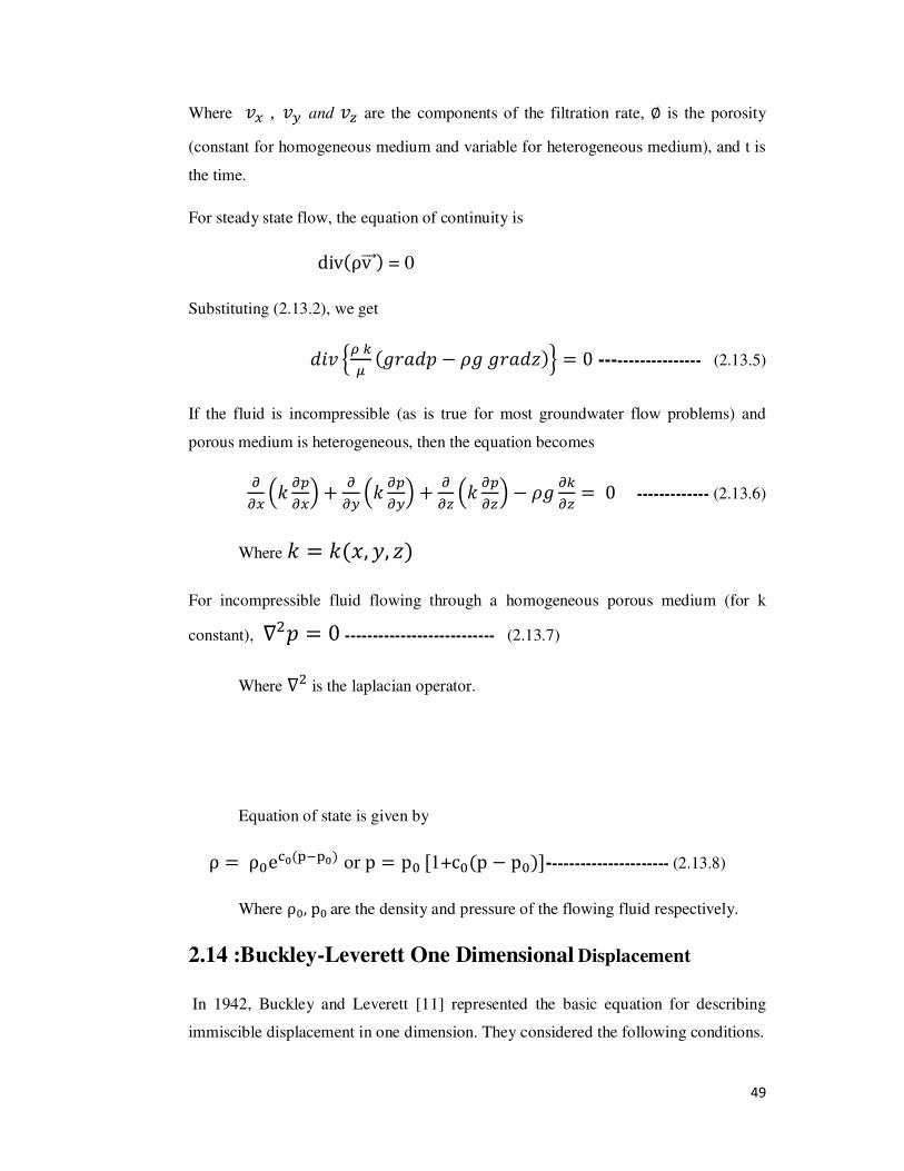
Where �� , �� and �� are the components of the filtration rate, ¨ is the porosity
(constant for homogeneous medium and variable for heterogeneous medium), and t is
the time.
For steady state flow, the equation of continuity is
div�ρv �� � = 0
Substituting (2.13.2), we get
��� ¤� �� ��\��� & ]� �\����§ � 0 ------------------ (2.13.5)
If the fluid is incompressible (as is true for most groundwater flow problems) and
porous medium is heterogeneous, then the equation becomes
��� $� ��
��( D ��� $� ��
��( D ��� $� ��
��( & ]� ���� � 0 ------------- (2.13.6)
Where � � ���, �, ��
For incompressible fluid flowing through a homogeneous porous medium (for k
constant), ©1� � 0 --------------------------- (2.13.7)
Where ©1 is the laplacian operator.
Equation of state is given by
ρ � ρle-���>��� or p � pl ª1+cl�p & pl�«---------------------- (2.13.8)
Where ρl, pl are the density and pressure of the flowing fluid respectively.
2.14 :Buckley-Leverett One Dimensional Displacement
In 1942, Buckley and Leverett [11] represented the basic equation for describing
immiscible displacement in one dimension. They considered the following conditions.
50
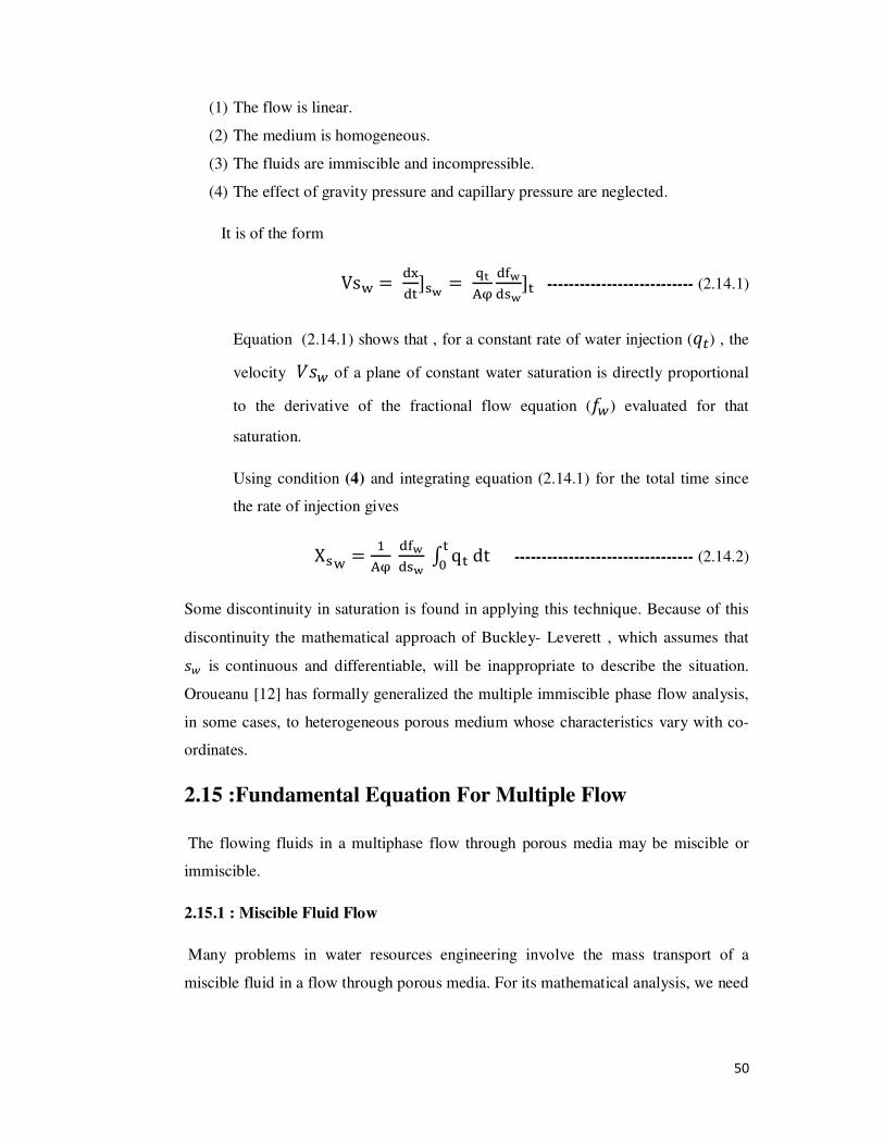
(1) The flow is linear.
(2) The medium is homogeneous.
(3) The fluids are immiscible and incompressible.
(4) The effect of gravity pressure and capillary pressure are neglected.
It is of the form
Vs¬ � �¥��«�R � T
A®��R��R«� --------------------------- (2.14.1)
Equation (2.14.1) shows that , for a constant rate of water injection (z ) , the
velocity �¯° of a plane of constant water saturation is directly proportional
to the derivative of the fractional flow equation (±°) evaluated for that
saturation.
Using condition (4) and integrating equation (2.14.1) for the total time since
the rate of injection gives
X�¬ � ?A® ��R
��R ³ q� dt�l --------------------------------- (2.14.2)
Some discontinuity in saturation is found in applying this technique. Because of this
discontinuity the mathematical approach of Buckley- Leverett , which assumes that
¯° is continuous and differentiable, will be inappropriate to describe the situation.
Oroueanu [12] has formally generalized the multiple immiscible phase flow analysis,
in some cases, to heterogeneous porous medium whose characteristics vary with co-
ordinates.
2.15 :Fundamental Equation For Multiple Flow
The flowing fluids in a multiphase flow through porous media may be miscible or
immiscible.
2.15.1 : Miscible Fluid Flow
Many problems in water resources engineering involve the mass transport of a
miscible fluid in a flow through porous media. For its mathematical analysis, we need
51
some fundamental equations governing the problem and certain condition, and
assumptions.
The equation of the continuity for the mixture is given by
¢]¢´ D µ · �]� ���·� � 0
Where ρ s the density for mixture and ����· is the pore (seepage) velocity (vector).
The equation for diffusion for a fluid flow through homogeneous porous media with
no addition or subtraction of the dispersing material is given by
¢]¢´ D µ · �¸� ���·� � µ · ¹]ºa µ :¸
]=»
Where c is the concentration of one fluid in other host fluid, Da is the tensor co-
efficient of dispersion with nine components D.F.In laminar flow, the equation of
continuity is given by (density is constant).
µ · � ��� = 0
and equation of concentration becomes
¢¸¢´ D � ��� · µ¸ � µ · ªºa µ¸«
2.15.2 : Immiscible Fluid Flow
Oil and water is the typical illustration of two immiscible fluid flows in porous
media. Further we call the fluid contained in porous medium by native fluid and the
fluid which is injected into the medium as an injected fluid. Since the unique feature
requiring a generalized treatment of multiple flow system is in the variability in the
phase distributions as the fluid progress along its macroscopic streamline, therefore
analytical description of such flows may be given by Darcy’s law applied to each
phase separately.
The relative velocity, in the Darcy sense, of phase j (native or injected fluid) is;
52
V�� �F � & k k�FµF ©pF D k k�F
µF ρFg ��
Where k�F the relative permeability of phase j is, © is the gradient symbol, �½ is the
pressure in phase j, and � ��� is the gravitational acceleration vector
The equation of continuity for the two immiscible phases given by
φ ∂∂t ¾ρFsF¿ D © · ¾ρFVÀ��� ¿ � 0
Where φ is the porosity, ρF is the density, and ½ is the saturation for phase j. “·”
symbolizes the scalar operation.
The pressure discontinuity (P-) between two phase is given by
P- � PZ&P.
The equation of state for the phase j may be written as ρF � ρF�PF�
From the definition of saturation, we have
s.D sZ � 1
All the above equations give the analytical basis of the two phase flow in a porous
medium.
2.16 : Physical Phenomenon
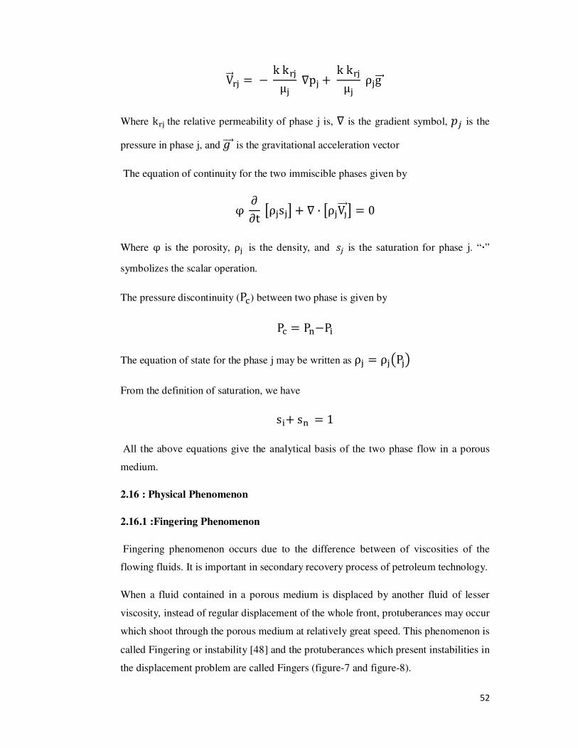
2.16.1 :Fingering Phenomenon
Fingering phenomenon occurs due to the difference between of viscosities of the
flowing fluids. It is important in secondary recovery process of petroleum technology.
When a fluid contained in a porous medium is displaced by another fluid of lesser
viscosity, instead of regular displacement of the whole front, protuberances may occur
which shoot through the porous medium at relatively great speed. This phenomenon is
called Fingering or instability [48] and the protuberances which present instabilities in
the displacement problem are called Fingers (figure-7 and figure-8).
53
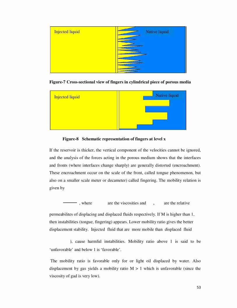
Figure-7 Cross-sectional view of fingers in cylindrical piece of porous media
Figure-8 Schematic representation of fingers at level x
If the reservoir is thicker, the vertical component of the velocities cannot be ignored,
and the analysis of the forces acting in the porous medium shows that the interfaces
and fronts (where interfaces change sharply) are generally distorted (encroachment).
These encroachment occur on the scale of the front, called tongue phenomenon, but
also on a smaller scale meter or decameter) called fingering. The mobility relation is
given by
, where are the viscosities and , are the relative
permeabilites of displacing and displaced fluids respectively. If M is higher than 1,
then instabilities (tongue, fingering) appears. Lower mobility ratio gives the better
displacement stability. Injected fluid that are more mobile than displaced fluid
), cause harmful instabilities. Mobility ratio above 1 is said to be
‘unfavorable’ and below 1 is ‘favorable’.
The mobility ratio is favorable only for or light oil displaced by water. Also
displacement by gas yields a mobility ratio M > 1 which is unfavorable (since the
viscosity of gad is very low).
Injected liquid Native liquid
Injected liquid Native liquid

54
Scheideger and Johnson [44] , first stabilize the fingers by introducing the concept of
statistical treatment of fingers, only the average cross-sectional area occupied by the
fingers has been considered and the size and shape of individual finger are
disregarded
In this case the saturation of the jth
(injected fluid) sF , is defined as the average
relative area occupied by it at level �.
i.e.sF � sF�x, t�, if the displacement processes are in � -direction with time t.
In the present analysis the following relationships suggested by Scheideger and
Johnson [13] has been considered.
kF � sF , kZ � sZ � 1 & sF
Where kF denotes fictitious relative permeability and. sF is the saturation of
phase j.
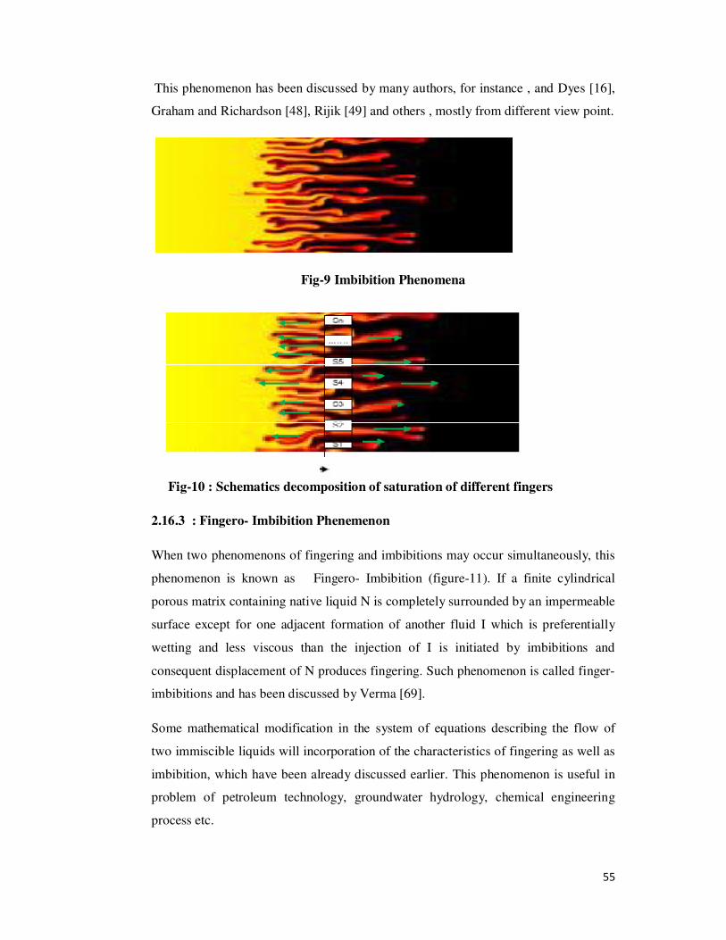
2.16.2 : Imbibition Phenomenon
The influence of capillary mechanism related to the porous media called capillary
imbibitions, is the spontaneous displacement of a non-wetting fluid. The phenomenon
of imbibition is due to the difference in wetting abilities of the flowing fluids. The
typical case of imbibition is the displacement of oil by water, and it represents a
favorable mechanism for oil- recovery.
When a porous medium filled with some fluid is brought into contact with another
fluid which preferentially wets the medium, and then there is a spontaneous flow of
the wetting fluid into the medium and a counter flow of the resident fluid from the
medium. Such phenomenon is known as imbibitions (fig-9 and fig-10). This
phenomenon has special significance in oil recovery where it can be responsible for
increased oil production up to 35% in some cases.
The mathematical conditions for imbibitions phenomenon is given by Scheidegger [2]
as follows:
� � �½ , where �½ is the seepage velocity of phase j.
55
This phenomenon has been discussed by many authors, for instance , and Dyes [16],
Graham and Richardson [48], Rijik [49] and others , mostly from different view point.
Fig-9 Imbibition Phenomena
Fig-10 : Schematics decomposition of saturation of different fingers
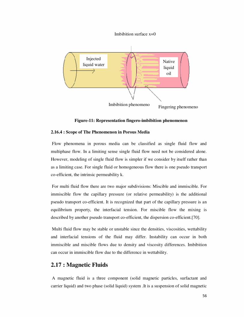
2.16.3 : Fingero- Imbibition Phenemenon
When two phenomenons of fingering and imbibitions may occur simultaneously, this
phenomenon is known as Fingero- Imbibition (figure-11). If a finite cylindrical
porous matrix containing native liquid N is completely surrounded by an impermeable
surface except for one adjacent formation of another fluid I which is preferentially
wetting and less viscous than the injection of I is initiated by imbibitions and
consequent displacement of N produces fingering. Such phenomenon is called finger-
imbibitions and has been discussed by Verma [69].
Some mathematical modification in the system of equations describing the flow of
two immiscible liquids will incorporation of the characteristics of fingering as well as
imbibition, which have been already discussed earlier. This phenomenon is useful in
problem of petroleum technology, groundwater hydrology, chemical engineering
process etc.
56
Figure-11: Representation fingero-imbibition phenomenon
2.16.4 : Scope of The Phenomenon in Porous Media
Flow phenomena in porous media can be classified as single fluid flow and
multiphase flow. In a limiting sense single fluid flow need not be considered alone.
However, modeling of single fluid flow is simpler if we consider by itself rather than
as a limiting case. For single fluid or homogeneous flow there is one pseudo transport
co-efficient, the intrinsic permeability k.
For multi fluid flow there are two major subdivisions: Miscible and immiscible. For
immiscible flow the capillary pressure (or relative permeability) is the additional
pseudo transport co-efficient. It is recognized that part of the capillary pressure is an
equilibrium property, the interfacial tension. For miscible flow the mixing is
described by another pseudo transport co-efficient, the dispersion co-efficient.[70].
Multi fluid flow may be stable or unstable since the densities, viscosities, wettability
and interfacial tensions of the fluid may differ. Instability can occur in both
immiscible and miscible flows due to density and viscosity differences. Imbibition
can occur in immiscible flow due to the difference in wettability.
2.17 : Magnetic Fluids
A magnetic fluid is a three component (solid magnetic particles, surfactant and
carrier liquid) and two phase (solid liquid) system .It is a suspension of solid magnetic
Imbibition surface x=0
Injected
liquid water Native
liquid
oil
Imbibition phenomeno Fingering phenomeno
57
particles of sub domain size in a liquid carrier. The fluid medium thus obtained is a
sort of colloidal dispersion.
Particles within the liquid experience a force due to the field gradient and move
through the liquid imparting drag to it causing it to flow. Thus, the magnetic fluids
can be made to move with the help of a magnetic field gradient, even regions where
there is no gravity.
2.17.1 : Fluid Dynamics Involving Magnetic Fluid
In classical (ordinary) fluid dynamics, there are only three forces viz. (i) the pressure
gradient (ii) gravity force (iii) the viscous force which have been taken account and
accordingly the equation of motion is stated as the sum of the gradients of all those
forces remains equal to rate of change of velocity multiplied by the density. Whereas
in case of Ferro hydrodynamics, the magnetic attraction; Vander Walls attraction;
static repulsion and electrical repulsion. Among which we have considered only two
namely magnetic body force and magnetic attraction. Since magnetic attraction is a
long range potential and varies very slowly with distance.
The magnetic body force originated from the interaction of magnetic field H with the
magnetization of the fluid and is of great importance regarding all further
investigation.[67].
2.17.2 : Basic Equations in Flow of Two Immiscible Fluids Through Porous
Media with Magnetic Fluid
Since the unique feature requiring a generalized treatment of the multiphase flow
systems is the variability in the phase distributions as the fluid progress along its
microscopic streamlines therefore analytical description of such flows may be given
by applying Darcy’s law to each phase separately. Assume that injecting fluid has a
layer of magnetic fluid and is regarded as pseudo single phase [68].
According to Darcy’s law, the basic flow equations of their simultaneous flow may
be given as
�� � & Ã�� Ä�Å Æ � ��\��_� D �\��Ç & ]��\��È�
58
� � & Ã� ÄÂÅ Æ � ��\��_ D �\��Ç & ]Â�\��È�
Where �� and � are the seepage velocities of displacing (injecting) and native liquids
respectively. �� �� � are the relative permeabilites of the injecting and native
fluid respectively. k is the total permeability. _� and _Â are the pressure of the
injected and native fluid respectively. And µ. and µZ are the viscosities of the injected
and native fluid respectively.
The equation of continuity for the two immiscible phases are :
X�¢ ¢´⁄ ��]�Ë�� � &����]����
X�¢ ¢´⁄ ��]ÂËÂ� � &����]Â�Â�
Where X is the porosity, ]� and ]Â are fluid density of injected and native fluid
respectively and S. and SZ are the saturation of the injected and native fluid
respectively.
The pressure discontinuity P- between the two phases is given by
P- � PZ & P.
The equation of state for the two phases may be written by
ρ. � ρ. �P.�
ρZ � ρZ �PZ�
From the definition of phase saturation, we have,
SZ D S. � 1
These equations are very difficult to analyze analytically due to their nonlinear
character and therefore, only approximate solutions have been obtained so far in
special cases and conditions. This system of equation modified by the special
conditions will be subject of subsequent investigations.
59
2.18 : Solution Techniques for Partial Differential
Equations (PDE)
2.18.1 : Partial Differential Equations
Consider the most general second order PDE
ÌÍ�� D 2ÏÍ�� D HÍ�� & Ç��, �, Í, Í�,Í�� � 0 ------------ (1)
1. Eq.(1) is called semi linear if A,B and C are functions of independent variable
�, � only.
2. Eq.(1) is called quasilinear if A,B and C are functions of �, �, Í, Í�,Í� .
3. Eq.(1) is called linear if A,B and C are functions of � �� � ,H is a linear a
function of Í, Í�, �É� Í�.
The most general second order linear PDE in two variables � �� � can be
expressed as
Ì��, ��Í�� D 2Ï��, ��Í�� D H��, ��Í�� D º��, ��Í� D Ð��, ��Í�D Ñ��, ��Í D Ò��, �� � 0
If G= 0, then PDE is called homogeneous otherwise inhomogeneous.
Classification of PDE
1. If B1 & 4AC � 0 , then parabolic.
e.g. Heat equation Í � �Í��
2. If B1 & 4AC Ö 0 then hyperbolic.
e.g. Wave equation Í � �Í��
3. If Ï1 & 4ÌH Q 0 then elliptic.
e.g. Laplace equation �� D �� � 0
2.18.2: Associated Conditions With PDE
60
The parabolic and elliptic type problems are always initial value problem whereas the
elliptic type problem is always boundary value problem. Initial value problem can be
further classified as pure initial value problem or initial boundary value problem.
(A) Pure Initial Value Problem(Cauchy Problem)
1. Í � �Í�� defined on &∞ Q � Q ∞ & ´ Ù 0 along with initial
condition Í��, 0� � ±���, &∞ Q � Q ∞
2. Í � �Í�� defined on &∞ Q � Q ∞ & ´ Ù 0 along with initial
condition
Í��. 0� � ±���, Í ��. 0� � ���)
(B) Initial Boundary Value Problem
Í � �Í�� defined on 0 Q � Q Ú & ´ Ù 0 along with initial condition
Í��, 0� � ±���, 0 Q � Q Ú and the boundary conditions at � � 0 & � � Ú.
The elliptic boundary value problem is classified depending on the boundary
conditions that are prescribed on the boundary.
There are three types of boundary conditions.
(a) Dirichlet/ First boundary condition:
The condition on which the solution of equation is prescribed along with a
boundary.
If elliptic problem is associated with Dirichlet boundary condition then it is called
Dirichlet boundary value problem.
e.g. �� D �� � 0 is defined on region R and boundary by C along with
boundary conditions Í��, �� � ±��, �� on C.
61
(b) Neumann/Second boundary conditions :
The conditions on which the derivative of the solution is specified along a
boundary. If elliptic problem is associated with this boundary condition then it is
called Neumann boundary value problem.
e.g. �� D �� � 0 is defined on region R and boundary by C along with
boundary conditions �Û� ��, �� � ±��, �� on C(normal derivative).
(c) Mixed/Third boundary conditions :
The conditions on which the solution and its derivative are prescribed along
the boundary. If elliptic problem is associated with this boundary condition
then it is called mixed boundary value problem.
e.g. �� D �� � 0 is defined on region R and boundary by C along with
boundary conditions Ü �S�u D β�s� ���Z � h�s� on C.
Well-Posed Problem: If solution exists, is unique and depends continuously on the
given data.
2.18.3 : Numerical Methods
When the equation describing the phenomena cannot be solved analytically then
solution can be obtained by numerical methods. The equation describing the
phenomena is to simulate the problem numerically. In simulation, the differential
equations are expressed with finite differences or polynomial solutions that match the
differential equations and explain phenomena with calculations via a computer. This
technique is called Numerical Modeling or Numerical Simulation.
As numerical method gives an approximate solution of given PDE, these
approximate values may contains the following error.
(1) Round off error: Difference of true representation of solution from machine
representation solution.
(2) Trunction error:Difference of exact solution from machine representation
solution.
62
Finite Difference Method
In FDM partial derivatives are replaced by finite differences at each node point. Most
common finite difference representation of derivative is based on Taylor’s series.
Conversion of partial derivatives in terms of finite difference [63].
Let Í�,½ denotes x-component of dependent variable at point��, Þ�
$�Û��(�.½ ß
�àáv,â>�à,â@ + o(h) (Forward difference)
ß �à,â>�àáv,â
@ + o(h) (Backward difference)
ß �àáv,â>�àUv,â1@ D o�h� (Central difference)
$�gÛ��g(�.½ ß �àáv,â>1�à,âã�àUv,â
�@�g + o(h2)
(Second order central difference)
$�Û��(�.½ ß
�à,âáv>�à,âb + o(k) (Forward difference)
ß �à,âáv>�à,,âUv
b + o(k) (Backward difference)
ß �à,,âáv>�à,,âUv
1b + o(k) (Central difference)
$�gÛ��g(�.½ ß �à,,âUv>1�à,âã�à,,âáv
�b�g + o(k2) (Second order central difference)
$ �gÛ����(�.½ ß �àáv,âáv>�àáv,âUv>�àUv,âávã�àUv,âUv
ä@b + o(k2)
(Second order central difference)
63
ååæ $ç�æ� åè
åæ(é.ê ß ëìíì ¾�çéãë,ê D çé,ê��èéãë,ê & èé,ê� & �çé,ê D çé>ë,ê��èé,ê & èé>ë,ê�¿
[Where ���� î ¸1& Í���î ¸ä]
STEPS TO SOLVE PDE BY FDM
(1) A rectangular grid is super-imposed on the region of interest as follows:
In one-dimensional case
�� � �l D �� , � � 0,1,2, … ………
Where h is the mesh size in the x-direction.
And ½ � Þ�, Þ � 0,1,2, … … … … … …. Where k is the step length in the t-direction.
The point of intersection are called nodes.
(2) Partial derivatives are replaced by difference quotients, converting differential
equation to the difference equation at each nodal point which is known as
Discretization of the given PDE.
(3) Difference equation and given data are used to determine the function values
at the nodes of the grid.
1. Gauss- Jacobi Method :
In this method the iteration formula expresses the �Þ D 1� w iterate in terms of the
Þ w iterates only.
2. Gauss- Seidal Method :
The method uses the latest iterative available and scans the mesh points systematically
from left to right along successive rows.
It can be shown that the Gauss-Seidal scheme converges twice as fast as the Jacobi
method. This method is also referred to as Leibmann’s method.
64
3. Crank- Nikolson Method:
In Crank and Nikolson proposed a method in which or is replaced by an average of its
finite difference approximation s on the �Þ D 1� wand Þ w level.
Consider the heat equation:
c ���� � �g�
�¥g , c being constant ----------------------------- (1)
Let (�,t) plane be divided into smaller rectangle by means of the sets of lines.
�� � �l D �� , � � 0,1,2,…..
tF � jk, j � 0,1,2, … ….
Using Finite difference analogue and Crank-Nikolson method for (1)
c $�àðáv>�àðb ( � ?1 Ã�àáv�ðáv�>1�à�ðáv�ã�àUv�ðáv�
@g D �àávð >1�àðã�àUvð@g Æ------(2)
&λu.>?,Fã? D �2 D 2λ�u.,Fã? & λu.ã?,Fã? � λu.>?,F D �2 & 2λ�u.,F D λu.ã?,F ------ (3)
Where λ � b-@g
Equation (3) is an implicit scheme, is called Crank-Nikolson formula and is
convergent for all finite values ofλ.
If there are N internal mesh points on each row, then formula (3) gives N
simultaneous equations for the N unknowns in terms of the given boundary values.
Similarly, the internal mesh points on all rows can be calculated.
4. Successive Over- Relaxation (or SOR) Method:
From equation (3), we have

65
�1 D λ�u.,Fã? � u.,F D λ2 ¾u.>?,Fã? D u.ã?,Fã? D u.ã?,F D u.>?,F & 2u.,F¿
--------------------------- (4)
Let ¸� � u.,F D ò1 ¾u.ã?,F D u.>?,F & 2u.,F¿------------------------ (5)
From (3), we have
u., � ó��?ãò� D ò1�?ãò� ªu.>? D u.ã?« ---------------------- (6)
u.,�Zã?� � ó��?ãò� D ò
1�?ãò� ªu.>?Z D u.ã?Z « -----------------------(7)
u.,�Zã?� � ó��?ãò� D ò1�?ãò� ôu.>?�Zã?� D u.ã?Z õ ------------------ (8)
Equation (7) is known as Gauss- Jacobi formula and (8) is known as Gauss- Seidal
formula.
It can be shown that the scheme (8) converges for all finite values of λ
And that it converges twice as fast as Jacobi scheme.
Equation (8) can be rewritten as
u.,�Zã?� � u.�Z� D ¤ ó��?ãò� D ò1�?ãò� ôu.>?�Zã?� D u.ã?Z õ & u.�Z�§ ------ (9)
From (9) it is clear that the expressions within the curly brackets is the difference
between the �É D 1� wand É w level.
From (8),
u.,�Zã?� � u.�Z� D ω ¤ ó��?ãò� D ò1�?ãò� ôu.>?�Zã?� D u.ã?Z õ & u.�Z�§
- -------------------(10)
Which is called successive over relaxation method. ÷ is called the relaxation factor or
accelerating factor and it lies , generally, between 1&2.
66
It was shown by B.A.Carre that for ω � 1.875 the rate of convergence of (10) is
twice as fast as whenω � 1, and for ω � 1.9 the rate of convergence is 40 times
greater than that whenω � 1. In general, however it is difficult to estimate the best
value of ω.
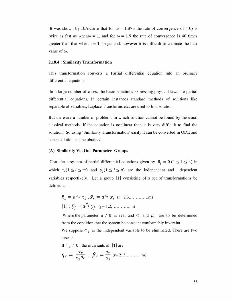
2.18.4 : Similarity Transformation
This transformation converts a Partial differential equation into an ordinary
differential equation.
In a large number of cases, the basic equations expressing physical laws are partial
differential equations. In certain instances standard methods of solutions like
separable of variables, Laplace Transforms etc. are used to find solution.
But there are a number of problems in which solution cannot be found by the usual
classical methods. If the equation is nonlinear then it is very difficult to find the
solution. So using ‘Similarity Transformation’ easily it can be converted in ODE and
hence solution can be obtained.
(A) Similarity Via One Parameter Groups
Consider a system of partial differential equations given by θF � 0 �1 ý i ý n� in
which ���1 ý � ý �� and �½�1 ý Þ ý É� are the independent and dependent
variables respectively. Let a group �1� consisting of a set of transformations be
defined as
��? � �Üv �? , ��� � �Ü� �� (r =2,3,………….m)
�1� : �c½ � ��� �½ (j = 1,2,…………..n)
Where the parameter � 0 is real and � and �� are to be determined
from the condition that the system be constant conformably invaraint.
We suppose Ü? is the independent variable to be eliminated. There are two
cases :
If Ü? 0 the invariants of �1� are
�� � ���v� , �� � �
v (r= 2, 3,………..m)
67
And ±½ ��1,��, … … �`� � �� ��v,……..,����v
��vÅ , �1 ý Þ ý É�
If Ü? � 0 and the simultaneous equations have a nontrivial solution, then we
may choose a group �2� consisting of
�?ccc � �? D ln � , ��� � �Ü� �� , �c½ � ��� �½
And the invariant group are
�� � ��p���Ü� �v� (r= 2, 3,………..m)
±½ ��1,��, … … �`� � �� ��v,……..,���p������v� , �1 ý Þ ý É�
(B) Similarity via Separable of Variables
Birkhoff [26] has introduced this method. When the method is applied one has to
assume the general form of similarity variable to begin with and in addition make all
substitutions into the equation. The resulting differential equations and the boundary
conditions must be examined before one obtains the specific similarity variables.


![1 lab physico-chemical_properties_of_drugs[1]](https://img.pdfslide.us/doc/110x75/55a8edea1a28abb32b8b4824/1-lab-physico-chemicalpropertiesofdrugs1.jpg)