Chapter 2 - National Institutes of Health · Web viewThe number stored for each voxel is an average of some physical parameter over the voxel’s volume. Since voxels are relatively

Appendix A. Setting Up an fMRI Scanning Session[This will be adapted from my handout in the June 1998 workshop.]

Appendix B. Safety Issues in MRI[Consult with Tom Prieto]

Appendix C. GlossarySome of these terms are not used in this book, but are defined here to help in reading the fMRI literature.

Acoustic NoiseWhen electrical current flows through a wire that is embedded in a magnetic field, there is a

force on the wire that is perpendicular to both the magnetic field and to the direction of the current flow. This force tends to move the wire and whatever it is attached to. If the current flow is reversed, the force will point in the opposite direction. The currents in gradient coils are large (about 100 Amperes) and they are embedded in large magnetic fields. In echo-planar imaging (EPI), the gradient currents are switched back and forth in direction about 1000 times per second. This produces a large alternating in-and-out force on the gradient coil structure, right at typical acoustic frequencies. The resulting vibration of the gradient coil is transmitted to the air and is audible, often painfully so.Acronyms

MRI physicists love acronyms. It seems that an imaging method isn’t complete until a funny- or profound-sounding acronym has been attached to it. Some examples:

DUFIS Dante UltraFast Imaging SequenceRAGE Rapid Acquisition with Gradient EchoesFLAIR FLuid Attenuated Inversion Recovery

Adiabatic RF PulseThis type of RF excitation pulse is used when precise slice selection is important. They work

particularly well when the B1 field is not uniform in intensity. The technique requires a longer time (20–30 ms, vs. 2–4 ms for normal RF pulses), which means that more radiofrequency energy is deposited into the subject with each transmission. This effect means that the repetition time (TR) with adiabatic pulses must be longer to keep the total SAR at safe levels. For this reason, adiabatic pulses are only used when necessary. One application is to slice selective 180 (inversion) pulses, which are hard to design accurately using simpler methods.ADC [Apparent Diffusion Coefficient]

Water molecules diffuse amongst themselves due to thermal motion. The self-diffusion coefficient (symbol: D) measures the rapidity of this mixing. D can be measured using MRI, since H2O molecules that move will carry their protons into regions with different magnetic field strengths, and so cause greater signal dephasing. However, what is really measured is the amount of H2O molecular mixing averaged over a voxel volume. Such mixing also occurs due to microscopic flows (as in capillaries), which increases the measured value of D over its true value. For this reason, the D that is measured with MRI in tissue is usually called the apparent diffusion coefficient (ADC).

In a layered medium, water molecules can diffuse more easily in some directions than in others. In the brain, water diffuses more easily down myelinated axonal fiber tracts than across them. This preferential diffusion can be detected using MRI, and promises to provide a method to trace white matter tracts noninvasively in vivo. Diffusion imaging has also proved useful in assessing cerebral damage due to stroke.

Robert W Cox Page 1 5/7/2023

ADC [Analog to Digital Converter]This device converts the voltage detected in the RF receive coil to numbers for storage in a

computer. One number is measured in each sampling interval (usually 1–10 s) for the duration of the readout window; the number of bits used to measure the voltage is called the sampling depth of the converter (usually 12–16 bits). This collection of numbers through time is then broken into frequency and phase components to reconstruct the actual image.AliasingTime series data is acquired in discrete steps, almost always uniformly spaced in time. The underlying processes are occurring in continuous time, being made up of components at all frequencies. Discretely sampled data cannot distinguish between all these frequency components. Denote the sampling time step by t. Then continuous time frequencies f and f(t)1 cannot be distinguished in the sampled data; for example, cos(0t) and cos(2tt) are identical at all times t=nt for integer n (both are equal to 1 for all n). This confusion of frequencies is called aliasing. Aliasing is the source of wraparound when the image FOV is smaller than the object being scanned. Aliasing also makes it difficult to separate high frequency heartbeat-related NMR signal changes from low frequency activation-related NMR signal changes, since the t for fMRI tends to be several seconds (e.g., t=4 s means that frequency aliasing occurs for frequencies above 0.25 Hz; heartbeat-related signals at 1.0–1.1 Hz will be aliased with signals in the range 0.0–0.1 Hz, which is the typical low frequency range of fMRI measurable activations).Amplifiers

An MR scanner contains many things called amplifiers. The gradient amplifiers produce the electrical current to run through the gradient coils (about 100 Amperes). The RF amplifier produces the radiofrequency waves transmitted to the RF coil, used to excite the magnetization. The RF receiver contains several amplifiers to boost the received NMR signal up to a level where it can be detected by the analog to digital converter.

It is important to understand that the actual numbers in the MRI voxels do not represent an absolute measurement. The entire RF receiver amplification system is designed to boost the NMR signal to a standard voltage range for digitization. This goal is accomplished by changing the receive amplifier gain to get the signal to the right level. The amplifier gain may be set by the scanner operator, or may be set automatically by the scanner software at the start of the scanning session. In either case, it is unlikely to be the same on two different days. Even if the amplifier gain were set consistently, the strength of the NMR RF signal is somewhat dependent on the exact position of the subject’s head and body relative to the RF receive coil, even for whole body coils. As a result of these complications, the BOLD effect is usually quoted in “percent signal change”, indicating that the voxel values rise 3% (say) above the resting baseline during an active task. Analyzing the results relative to the baseline removes the issue of the inter-session variability in NMR signal amplification.Angiography [MRA]This term refers to a set of MRI techniques that are designed to allow detection of blood vessels. All such techniques rely on changes that occur in the NMR signal when the H2O protons are flowing rather than standing still (or just diffusing). Vessels smaller than about 1 mm in diameter cannot be detected reliably with MRA techniques. The term “venography” is sometimes used when MRA methods are applied to detection of veins.Arterial Spin Labeling [ASL]

About 70% of the H2O molecules that enter a cerebral capillary diffuse through tiny pores and end up in the brain parenchyma (water in the brain diffuses back to replace the water in the capillaries).


If the water in the base of the brain were labeled, then the blood in the major arteries would flow up to the capillaries and most of it would exchange to the parenchyma. Detection of this label would provide a measure of the amount of tissue perfusion, since there is relatively little water “leakage” from larger vessels in the brain. Positron emission tomography (PET) works by using 15O labeled water as a radioactive tracer. ASL is an MRI technique where magnetization inversion is used to provide the labels; a slice-selective RF 180 pulse at the base of the brain flips the magnetization over. When these protons reach the parenchyma, their magnetization will be different from those protons that were not inverted. The resulting difference in the NMR signal can be used to estimate the amount of water that was transported from the base of the brain to the cerebral tissue.

There is a number of different imaging methods used for ASL, including: EPISTAR [???], FAIR [???], and QUIPPS [???]. The main drawback to all ASL techniques is the relatively small signal change that survives after all the magnetization processing that takes place.Artifact

This is a catch-all term used by MRI physicists to denote anything that corrupts or distorts an image. Anything that affects the static magnetic field, the RF magnetic field, or the subject in the scanner is likely to affect the image. In some cases, artifacts can be used to measure interesting physiological or physical properties. For example, the self-diffusion coefficient D of water increases with temperature; this artifact is one way to map temperature in vivo using MRI (it’s accurate to about 1 C).Asymmetric Spin Echo (ASE)—see Gradient EchoAxial

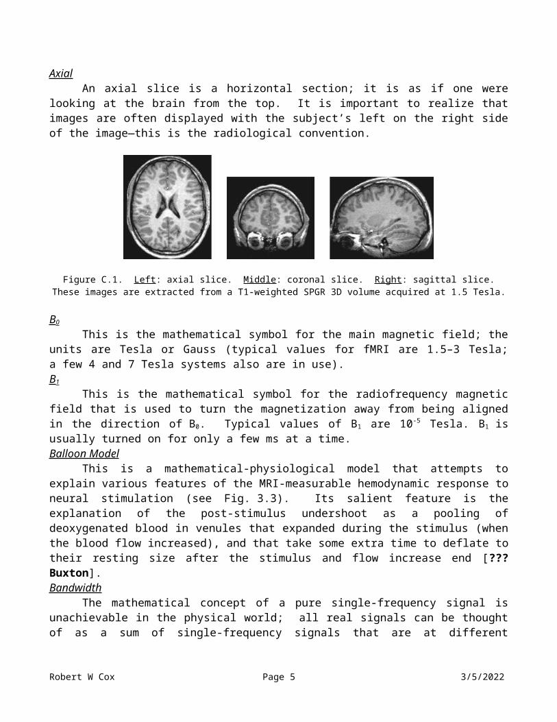
An axial slice is a horizontal section; it is as if one were looking at the brain from the top. It is important to realize that images are often displayed with the subject’s left on the right side of the image—this is the radiological convention.

Figure C.1. Left: axial slice. Middle: coronal slice. Right: sagittal slice.These images are extracted from a T1-weighted SPGR 3D volume acquired at 1.5 Tesla.

B0

This is the mathematical symbol for the main magnetic field; the units are Tesla or Gauss (typical values for fMRI are 1.5–3 Tesla; a few 4 and 7 Tesla systems also are in use).B1

This is the mathematical symbol for the radiofrequency magnetic field that is used to turn the magnetization away from being aligned in the direction of B0. Typical values of B1 are 10-5 Tesla. B1 is usually turned on for only a few ms at a time.


Balloon ModelThis is a mathematical-physiological model that attempts to explain various features of the MRI-

measurable hemodynamic response to neural stimulation (see Fig. 3.3). Its salient feature is the explanation of the post-stimulus undershoot as a pooling of deoxygenated blood in venules that expanded during the stimulus (when the blood flow increased), and that take some extra time to deflate to their resting size after the stimulus and flow increase end [??? Buxton].Bandwidth

The mathematical concept of a pure single-frequency signal is unachievable in the physical world; all real signals can be thought of as a sum of single-frequency signals that are at different frequencies. The bandwidth of a real signal expresses the range of frequencies that are included in the signal. For example, a standard television signal in the USA has a bandwidth of 4.3 MHz; that is, the smallest frequency present in the signal is 4.3106 Hz smaller than the largest frequency. The bandwidth of the NMR signal received in human brain imaging usually ranges from 60 KHz to 250 KHz—this bandwidth is determined by the gradient strength and the size of the subject.BOLD [Blood Oxygenation Level Dependent]

This acronym refers to the discovery that the NMR signal strength received from a voxel containing blood depends on the amount of oxygen in the blood [??? Thulborn, Ogawa]. This effect is the foundation of fMRI, since blood oxygen level increases locally during neural activity. The cause of the BOLD effect is the change in microscopic magnetic field randomness as the iron atoms in blood hemoglobin molecules bind to oxygen (decreasing magnetic field randomness, since the susceptibility of oxyhemoglobin is the same as other soft tissue) or become unbound from oxygen (increasing magnetic field randomness, since the susceptibility of deoxyhemoglobin is different from other soft tissue)—see Fig. 3.1.Bore

This term refers to the diameter of the main field magnet. For whole-body human imaging, the bore size is usually 90–100 cm. The actual usable space inside the magnet is usually smaller due to the extra equipment inside the main magnet cylinder (i.e., shim, gradient, and RF coils built into the walls).Carrier Frequency

This is the central frequency present in any real signal. In MRI, the carrier frequency for the NMR signal transmitted to and received from the protons is equal to 42.54 MHz times B0; at the widely used field strength of 1.5 Tesla, this is about the same frequency as television channel 4.Chemical Shift

The frequency at which a particular proton precesses is determined by the magnetic field strength at that proton. The electrons surrounding the protons may cause the externally imposed magnetic field (B0) to be slightly altered at the atomic nucleus. The amount of this alteration depends on the configuration of the electrons, and is different for different hydrogen-containing chemical compounds. For example, the methyl CH3 groups in fat molecules “see” a different magnetic field than the H2O molecules of water, and so resonate at a slightly different frequency. In NMR spectroscopy and spectroscopic imaging, it is possible to use the chemical shift to detect the concentrations of several different molecular species. (The chemical shift in frequency is larger when B0 is bigger, which is one reason for the drive to ever increasing magnetic fields.)CNR [Contrast to Noise Ratio]—see SNRCoherence

When dealing with several time-varying phenomena at the same time (e.g., multiple measurements), the different time series are said to be coherent if knowledge of one phenomenon at a


given time helps to predict the others at that time. This is a similar concept to correlation, but coherence can also be calculated as a function of frequency. For example, Biswal has shown that resting-state fMRI time series data from the left and right primary motor cortex areas are coherent at low frequencies (< 0.1 Hz) and incoherent at high frequencies [??? Biswal].Coil

Magnetic fields are created by electric currents in coils of wire, and are detected by the currents they generate in coils of wire. Gradient coils are arrangements of wire designed so that when current is applied, the resulting magnetic field strength varies spatially—in the x-, y-, and/or z-directions. RF coils are used to transmit and receive radiofrequency magnetic fields (exciting magnetization and detecting it, respectively). For practical reasons, the RF coil must be inside the gradient coil, since transmitting radio waves through a metal structure to get to the subject can cause serious electrical problems. The RF coil can also be thought of as an antenna that is tuned to operate at the resonant frequency of the magnetization. In some situations, separate RF coils are used for the transmitter and receiver.

Coils can be built into the bore of the scanner, so that they are not readily visible. This type of coil is called a body coil, since the subject’s entire body goes inside them. Coils can also be smaller and removable, and designed to fit over just a portion of the body. This type of coil is called a local coil. If a local gradient coil is used, then a local RF coil is needed for reasons explained above; however, a local RF coil can be operated with the body gradient coil, if desired.Complex Number

A complex number is defined as any number of the form , where a and b are standard real numbers. In the mathematical analysis of MRI physics, the separately measured I and Q components of the raw NMR signal are usually combined into one complex number, with a=I and b=Q. The reconstructed MR images contain a complex number in each voxel, but the final output is usually just the magnitude in each voxel: . Some imaging methods also use the phase of the image values: ; the phase is used in some forms of angiographic imaging and in measuring the magnetic field.Contrast

This term expresses the concept of a difference in NMR signal strength between two different types of tissue, or between the same tissue in two different conditions. The flexibility of MRI allows different physical and physiological properties to be enhanced with different imaging methods. Some examples of important contrast are:

T1 contrast Distinguishes gray and white matter in the brain (e.g., as in Fig. C.1)T2* contrast Via the BOLD effect, distinguishes more and less neurally active tissueFlow contrast Used in MR angiography to emphasize moving tissue, especially blood

Contrast AgentThis is a chemical compound given to the patient in order to enhance the NMR signal differences

between tissue types. These agents work by incorporating atoms that have a large intrinsic magnetic field (e.g., iron, gadolinium, dysprosium). Water molecules near these agents will experience a shift in the magnetic field, which will affect the T1, T2, and/or T2* relaxation time of the protons’ magnetization. (One can think of deoxyhemoglobin as an intrinsic contrast agent; hence the BOLD effect.) Although the first fMRI experiment was done with a external contrast agent [??? Belliveau], this type of experiment has not been repeated often in humans. Contrast agents are mostly used for detection of tumor and other pathologies; for these purposes, they are used millions of times per year.Convolution

A relationship between functions of one of the forms below is called a convolution:


r(t) is said to be the convolution of h(t) with s(t). This type of relationship is often used to model the response r(t) of a system to input stimuli s(t); the function h(t) is called the system’s impulse response function, and represents the output of the system to a brief stimulus occurring at time t=0. If r(t) is measured and s(t) is known, then the process of solving for h(t) is called “deconvolution”. For many systems, this is quite a sensitive operation; one whose results can be strongly contaminated by noise or slight changes in assumptions.Coronal

A coronal slice is a vertical section; it is as if one were looking at the brain from the subject’s front (see Fig. C.1).Correlation Method

This is the name of a widely-used method for detecting functional activation from fMRI time series data. The technique is to find the correlation coefficient between a user-specified time series that is presumed to model the time course of neural response to the known stimulus time course, and the NMR data time series from each voxel. Voxels with a large correlation coefficient are presumed to be “active”. (See chapter 7 for more details.)Crushers, Killers, and Spoilers

When an RF pulse is transmitted into the subject, the usual intention is create transverse magnetization in a certain slice and that has certain properties. If there is any pre-existing transverse magnetization, it will interfere with these goals. Crushers (etc.) are large bursts of current applied to the gradient coils whose goal is to dephase any existing transverse magnetization so that it won’t interfere with the transverse magnetization that is about to be created by a new RF pulse.Degree of Freedom (DOF)

A statistical term that (roughly speaking) measures the number of independent random samples in the analysis of a set of measurements. If the noise in each measurement is uncorrelated with all others (“white noise”), then the number of degrees of freedom is the number of measurements minus the number of parameters being fit in the analysis. Given a fixed level of a statistical parameter (e.g., a t-statistic or a correlation coefficient), the statistical significance of the parameter becomes higher—the p-value decreases—as the number of degrees of freedom increases. When the measurement noise is not white, the number of degrees of freedom is sometimes adjusted (reduced) to make the calculations of statistical significance be more correct.Dephasing [Destructive Interference]

The signal detected in the RF coil is the sum of all the signals emitted from magnetized protons all over the brain. If these component signals are positively coherent, then they will add up to a large value. If these component signals are random, then they will tend to cancel out, since about as many will be positive as are negative. At the moment transverse magnetization is created, all its components are positively coherent (in-phase). Since different regions of the brain will have slightly different magnetic fields, their transverse magnetizations will precess at slightly different frequencies. When enough time has passed, all the component signals will be incoherent (out-of-phase) and no NMR signal will be detectable (see Fig. 2.7). This process can be accelerated by the application of crusher gradient fields, which will enlarge the inter-regional magnetic field differences.Diamagnetic—see Susceptibility


DiffusionThis term describes the concept of molecular motion due to random thermal agitation (vs. motion

caused by flow or other non-random collective movements). In MRI, the most important diffusing substance is water, which diffuses easily due to its low molecular weight.Echo—see Gradient Echo and Spin Echo Eddy Current

The magnetic fields from the gradient coil not only penetrate inwards to include the subject, but also propagate outward. As they change in time, these external gradient fields induce extra currents in the superconducting coils of the main magnet (or in other nearby conductive surfaces)—these are referred to as eddy currents. Eddy currents in turn generate changes in the magnetic field back in the subject. These changes are unwanted and interfere with the imaging process, particularly with high speed imaging methods such as echo-planar imaging (EPI), where the gradient fields are changing rapidly and continually. The effects of eddy currents are smaller in large bore magnets, since the distance between the gradient coil and the main coil is farther. Another technique to reduce the effect of eddy currents is to build an “anti-coil” (or “active shield”) outside the gradient coil. This anti-coil operates in parallel with the gradient coil and is intended to produce an approximately opposite magnetic field at the main coil. The main drawback to this active shielding approach is that the opposite field also penetrates the subject, tending to cancel some of the gradients needed for imaging.EPI [Echo-Planar Imaging]

This term describes a very fast method for acquiring NMR image data: 40–100 ms per 2D image. EPI requires a gradient power supply and gradient coil combination that can be switched from positive to negative currents repeatedly and very rapidly (unlike most other imaging methods). Until relatively recently, this type of hardware was uncommon, but since the advent of fMRI, EPI capabilities have become more usual (but can still be expensive, particularly with whole body gradient coils). EPI is the most widely used acquisition technique in fMRI due to its high speed, which makes it possible to gather a whole brain volume every 2–4 seconds.Ernst Angle

After an RF pulse is applied, the pre-existing longitudinal magnetization is partly converted into transverse magnetization (the detectable component). If the flip angle is , then the fraction that remains as longitudinal magnetization is cos() and the fraction that is converted to transverse magnetization is sin(). If = 90, then all the longitudinal magnetization is converted into transverse magnetization. One might think that this would give rise to the largest possible NMR signal; however, this conclusion ignores the fact that many RF excitations will be used and the important thing is to have a large average signal over each separate readout. Suppose that the RF excitations hit a particular slice very rapidly (i.e., TR is short). Then the longitudinal magnetization that is the source of the transverse magnetization will have little time to recover (T1 relaxation). If = 90, the result is that there will be little NMR signal to measure at the second and subsequent readouts. Paradoxically, a smaller can actually result in a larger signal in the later readouts, since each time we are saving some longitudinal magnetization for later use. The Ernst angle is the optimum flip angle for a given TR, in that it produces the largest NMR signal over many RF pulse/readout combinations: Ernst = cos-1(eTRT1).Excitation

If left alone long enough (about 10 seconds), all the magnetization created by the main field will be aligned with the direction of the main field. In this condition (pure longitudinal magnetization), there is no precession of the magnetization, and there is no NMR signal that can be detected. The process of turning longitudinal magnetization to point at an angle to the main magnetic field is called excitation. It


is accomplished by applying a tiny magnetic field (B1) perpendicular to the main field and oscillating it at the same frequency that the magnetization precesses at.Fat Suppression

The signal from protons in CH3 groups in fat is at a slightly different frequency than the signal from protons in H2O. In MRI, position is determined by frequency, so that the image of fat will be somewhat displaced from the image of water. For most imaging methods, this is unimportant, since the bandwidth of the methods is much larger than this chemical shift. However, for EPI, the bandwidth in the phase-encoding direction is so low that the fat appears displaced several centimeters from its true location relative to the water. To get good echo-planar images, it is necessary to suppress the NMR signal from CH3 before the water signal is excited. This is done by using an RF pulse with carrier frequency centered at the CH3 frequency and with a bandwidth narrow enough to miss the H2O frequency. The result is that the CH3 protons are excited to transverse magnetization, which is then removed (completely dephased) with a crusher pulse.FID [Free Induction Decay]

After RF excitation, if the transverse magnetization is left undisturbed (i.e., no gradients applied and no more RF), then the measurable signal starts off large and will decay steadily to zero over an interval of about 3T2*. “Induction” is the electromagnetic term for the current induced in the RF receiving coil when the magnetization inside is changing. “Free” refers to the unmanipulated nature of the magnetization. In this situation, the recorded NMR signal is sometimes referred to as an FID, although the term really refers to the process rather than the result.Field

This term just refers to a physical quantity or parameter that is defined at every point in a spatial region. For example, the magnetic field created by the main magnet permeates space; its strength and direction vary from point to point. This is why it is called a “field”. In contrast, the speed of a car is not called a field, since it is a quantity that is attached to a single object.Field Map

In MRI, this term refers to an image whose voxel values are proportional to the magnetic field intensity difference from B0 at each location. The most common method for acquiring a field map is to acquire two images with identical methods except for different TEs; the phase difference between the complex numbers in the images yields the desired field map (after a little post-processing).FFT [Fast Fourier Transform]

The FFT is a collection of clever algorithms for computing a digital approximation to the Fourier transform quite rapidly. (If Cooley and Tukey—inventors of the first FFT algorithm [??? Cooley]—got 1¢ royalty for each FFT performed, they would now own the world. Being honorable mathematicians, they donated the algorithm to the world.)FLASH [Fast Low Angle ???]

This is a relatively rapid imaging method: about 600–1000 ms per 2D slice (approximately 10 times slower than EPI). It has been used for fMRI, but mostly at sites where EPI is not available. It is not practicable to do whole brain fMRI with FLASH, since about 20 slices are needed to cover the cerebrum, and about 50 images per slice are needed to compute decent functional activation maps.Flip Angle

If left alone long enough (about 10 seconds), all the magnetization created by the main field will be aligned with the direction of the main field. When disturbed by an RF pulse, the magnetization will point in a different direction. The angle between the magnetization before the RF pulse and after the RF pulse is called the flip angle.


Fourier TransformThe application of gradient fields after the excitation means that the frequency of the signal

emitted by the magnetization depends on its location. The signal detected at the RF coil is the sum of all the signals emitted from the excited tissue, so the recorded data will contain a mix of frequencies. These data must be broken down into their frequency components, each of which is then assigned to the appropriate location in the final image. The mathematical operation that transforms data recorded in time to their frequency components is called the Fourier transform. For this reason, MRI is sometimes called a Fourier imaging method, since the raw data do not comprise an image, but are the Fourier transform of an image.FOV [Field of View]

This term denotes the physical size of the imaged region, which is determined by the sampling rate in k-space, and thus is set by a combination of the analog to digital conversion rate and the gradient field strength. FOV can be specified at the scanner console directly (the scanner computer determines the necessary physical parameters for you). It is important to set the FOV to be large enough to encompass all the tissue in the slices being imaged. If there is tissue outside the FOV, it will not be unseen in the image. Instead, it will wrap back around the other side of the image, and overlap with the desired tissue. This happens when the sampling rate in k-space is too coarse, meaning that the Fourier transform can’t tell some frequencies apart. (This frequency confusion effect is also called “aliasing”.)Frequency

When a signal is oscillating periodically in time, the number of periods it cycles through in a unit time is called the oscillation frequency. The units of frequency are Hertz (cycles per second); KHz is the abbreviation for 1,000 cycles per second; MHz is the abbreviation for 1,000,000 cycles per second. Some examples:

Respiration about 0.25 HzHeartbeat about 1.1 HzEPI gradients about 1000 HzRF signals 42.54 MHz per Tesla of B0 (for protons)

Frequency EncodingThe measured NMR signal is the sum of all the signals emitted from all the magnetically excited

tissue. To be able to distinguish source locations in the measured signal, the components are made to differ in frequency by making the magnetic field strength vary with location. This is called frequency encoding. The Fourier transform provides a way to break the signal, measured as a function of time, into its different frequencies. As a result, the magnitude of each frequency component can be assigned to the location from which it originated (since the relationship between frequency and position is known). This type of spatial encoding only provides one dimension of the needed localization. The other two dimensions are provided by phase encoding and by slice selective excitation.Fully RelaxedThe condition that magnetization reaches when it is undisturbed by RF pulses for an interval at least 5T1 in length. The longitudinal magnetization reaches its maximum value, and the transverse magnetization goes to zero.FWHM (Full Width at Half Maximum)This term is used to describe the shape of a point spread or impulse response function. It is the distance (or time) between the points on the function where the function value is half of its maximum. This number describes the distance (or time) over which an impulse input affects the output. This number is


often taken to be the resolution of the system, since two input impulses closer than the FWHM will be blurred together in the output and will be indistinguishable.

Figure C.2. Definition of FWHM for a sample response function.

GaussAn older unit for the strength of a magnetic field; 1 Gauss equals 10-4 Tesla. The Earth’s

magnetic field is about 0.5 Gauss (except near the North and South magnetic poles). Abbreviation: G.Gaussian Noise

Noise whose sample values follow a Gaussian distribution. Separate values of Gaussian noise do not need to be independent (uncorrelated)—Gaussian noise should not be confused with white noise.Ghosts

In MRI, position is deduced from the frequencies and phases of the detected NMR signal. Unmeasured imperfections in the scanning process can cause the frequencies and phases of some components of the signal to be corrupted. These components will then be reconstructed to the wrong locations. These artifacts are usually faint, and so are called “ghost images”. Echo-planar imaging is particularly prone to ghosting, especially if the magnetic field is poorly shimmed.Gradient Echo

The application of a gradient field to the subject will cause the transverse magnetization to dephase, and the total NMR signal will decay away. Reversing the direction of the gradient field (e.g., changing the sign of Gx) will cause the dephasing to be undone, and the NMR signal will grow back. This effect is called a gradient echo. Imaging of the NMR signal relies on reading out the signal strength during the decay and/or echo intervals while gradient fields are applied. Gradient echoes can be made to coincide with spin echoes—this is the normal technique used in spin echo imaging. When a spin echo is created, but the gradient echo used in image acquisition does not coincide in time with the spin echo, this is called an asymmetric spin echo (ASE).Gradient Field

The precession frequency of the magnetization at location x is proportional to the magnetic field strength B(x) at that location. By making B(x) = B0 + Gx for some nonzero constant G, the frequency depends on location x; this is the mechanism that allows the total NMR signal to be separated into components that came from different locations. The magnetic field Gx is called the x-gradient field. For 3D imaging, gradient fields in the y- and z-directions are also needed, so that the total static magnetic field imposed by the scanner takes the form B(x,y,z,t) = B0 + Gx(t)x + Gy(t)y + Gz(t)z. The


strengths of the gradient fields are determined by the amount of current sent into the gradient coils. Typical values for the gradient strengths are 10 mT/m (= 1 G/cm).Hard and Soft RF Pulses

A “hard” RF pulse is one applied without magnetic field gradients turned on. In this case, the resonant frequency of all the protons inside the RF coil is the same, and they are all “flipped”. This is also called “whole volume excitation”. A “soft” RF pulse is one that is designed to keep to a narrow frequency band, and is applied at the same time a magnetic field gradient is turned on. The result is that only some of the region inside the RF coil is resonant with the RF pulse, and only the magnetization inside the resonant region is affected by the RF pulse (see Fig. 2.9).Hematocrit [Hct]

Volume fraction of the blood that is occupied by whole red blood cells. It is often used as a indicator of blood oxygen carrying capacity.Hemodynamic

An adjective used to describe changes in blood flow, volume, oxygenation, etc., in response to other physiologic events. Changes in neural activity do not measurably influence the NMR signal, but these type of changes in blood are visible in MR images, and can be caused by neural activity—hence, fMRI.Hemodynamic Response Function [HRF]

Many fMRI data analysis methods explicitly or implicitly assume that the NMR signal response to neural stimulation can be described by the superposition of a basic response h(t) that starts at the instant of stimulus. If two stimuli are separated by 3 s, then the model response is h(t)+h(t3). (Causality implies that h(t) = 0 for t < 0.) A popular model function is h(t) = t8.6et/0.547 [??? Cohen]. This function reproduces the stimulus onset delay, the time to maximum response, and the decay back to baseline reasonably well, and has the advantage that it is easy to program (unlike the balloon model, say). The hemodynamic response function is the temporal point spread function for the mapping from neural stimulation to fMRI time series.Hertz—see FrequencyI and Q—see QuadratureImpulse Response FunctionThe measured response of a system to an infinitesimally brief stimulus (an “impulse”). When the stimulus is longer, the system’s response is modeled to be the sum (or integral) of time-shifted copies of the impulse response function, each copy originating at the time of its corresponding stimulus. This concept is the time-domain analog of the point spread function.Inversion

If the flip angle of an RF excitation pulse is set to 180, it is sometimes called an inversion pulse. The effect is to turn longitudinal magnetization upside-down; that is, to anti-align it with the main magnetic field. Transverse magnetization is rotated 180 in the transverse plane. These effects have a large number of uses in MRI, including the generation of spin echoes.Inversion Recovery [IR]

Spin echoes are formed by first flipping the magnetization by 90, waiting, and then applying a 180 flip. Inversion recovery imaging works in the opposite way: longitudinal magnetization is flipped by 180, the pulse sequence waits, and then a 90 flip creates transverse magnetization, which is then used to form an image. During the 180–90 waiting period, the upside-down longitudinal magnetization will begin to relax back to the aligned state. By choosing the wait time (TI) properly, the resulting image can be very sensitive to the T1 values in tissue (i.e., very T1-weighted). Also, since M z migrates


from negative to positive, at some point in time it goes through zero. By choosing TI appropriately, tissue with any given value of T1 can be completely removed from the image. In brain imaging, this nulling is usually applied to cerebrospinal fluid. A double inversion recovery method can be used to remove two different values of T1; with this technique, it is possible to make a gray matter only or a white matter only image of the brain. [??? Redpath]Isocenter

This is the spot inside the magnet bore where the main magnetic field is most uniform. If you are using a local gradient coil, it should be centered around this location.k-space

“k” is the mathematical symbol used for coordinates in the Fourier transform. For this reason, MRI physicists often refer to the raw data as being acquired in k-space, which then must be transformed back to “real-space” for image display.Larmor Frequency

This denotes the frequency at which transverse magnetization precesses about the direction of the magnetic field. For magnetized protons, the Larmor frequency is B 42.54 MHz. The phrase “resonant frequency” is used interchangeably with this term.Localizer

During a scanning session, it is necessary to prescribe the desired slices in some way. A localizer is a quick 2D image taken perpendicular to the plane of the desired images (e.g., if you are going to gather axial slices, the localizer would be sagittal or coronal). From the localizer, it is easy to pick out the anatomical coverage desired by the subsequent image acquisitions.Magnetic Field

A magnetic field is defined by its effects on small magnets (or magnetizable materials, such as iron): it tends to align magnets placed in the field in a particular direction (see Fig. 2.1). The strength of the field determines the torque that the test magnets experience; the direction that the test magnets become aligned with defines the direction of the magnetic field. In MRI, the total magnetic field is the sum of many independently generated components: the main field, the gradient fields, the RF field, and the complex inhomogeneous field generated in the subject by susceptibility effects.Magnetization

Protons by themselves, as in a hydrogen nucleus, are slightly magnetic. When immersed in a large magnetic field, protons tend to line up with this field (see Fig. 2.2). As a result, water (H2O) in a magnetic field becomes slightly magnetized. The term magnetization refers to the amount of magnetism that is created at any given location; for example, tissue with a higher density of water will have a larger magnetization.

Magnetization is a vector field: it has a strength and points in a direction, and the strength and direction both can vary with spatial location (see Fig. 2.3). The symbol for vector magnetization is M. The component of magnetization that points along the main magnetic field direction is called longitudinal magnetization (symbol: Mz). Mz is not directly detectable. The component of magnetization perpendicular to the main magnetic field direction is called transverse magnetization (symbol: Mxy). Mxy is detectable, since it precesses rapidly about the direction of B0; this produces a tiny rapidly changing magnetic field, which induces a tiny rapidly changing voltage in the nearby RF receive coil.Magnetization Transfer [MT]

To contribute to the directly measurable NMR signal, hydrogen nuclei must be in molecules that vibrate and move rapidly (this effect is called “motional narrowing”). For the most part, this mean H2O


molecules and CH3 groups in fats; hydrogens in proteins and other large molecules are too rigidly bound to contribute to the measured signal—the result is that the T2 of protein protons is only about 10 s, and their NMR signal decays away before it can be measured at all. However, it is possible for such macromolecules to indirectly influence the NMR signal. Their 1H nuclei still become magnetized. When an H2O molecule come close to a protein, the magnetization state of the water protons can exchange with the protein protons. The magnetization of the protein protons is completely dephased, so when it transfers to the water protons, it does not contribute to the NMR signal. The magnetization of the water protons becomes completely dephased within microseconds of exchanging to the protein protons. The net effect is a diminishing of the NMR signal—the magnetization transfer (MT) effect. The MT effect is normally not large, but can be enhanced by using special RF pulses designed to flip the protein protons’ magnetization along with the water protons’ magnetization. MT imaging has not been used much in fMRI, but has some applications in clinical scanning (e.g., detection of multiple sclerosis lesions).Main Field

This is the huge magnetic field produced by the superconducting current—typical strengths for fMRI are 1.5–3 Tesla. Fields up to about 0.3 Tesla can be produced by permanent magnets or currents in normal resistive wire, but larger fields require such large currents that superconductors are the only available technology. The symbol for the main field is B0.

The main field magnetizes the protons in the tissue and creates the magnetization. The main field also causes the magnetization to precess (i.e., rotate, or spin) about the direction in which B0 points, at a speed that is proportional to the main field magnitude (see Fig. 2.3). The region inside the magnet where the main field is spatially uniform is called the “sweet spot” of the system. The middle of the sweet spot is the magnet’s isocenter.

Spatial uniformity in the main field is important for (at least) three reasons. The first is that frequency is used to encode spatial position, by the application of magnetic field gradients. The relationship between frequency and position must be known for this technique to work. The second reason is that a nonuniform magnetic field would increase the transverse relaxation rate (i.e., decrease T2*), and so the NMR signal would decay away faster. The third reason is that a larger range of magnetic field strengths would mean that a larger range of frequencies would be present. The NMR signal would have a larger bandwidth, which would require enlarging the RF receiver bandwidth. That would in turn increase the thermal noise level in the received NMR signal, which would degrade the image quality.Matrix

In MRI jargon, the image acquisition matrix is the size of the k-space grid on which the raw data are measured. The most common matrix used in EPI has been 6464. Normally, an image is reconstructed onto a grid that is the same size as the acquisition matrix, but this is not necessary.

In mathematics, a matrix is a set of numbers that represents a linear transformation of a vector; for example, rotation of coordinates can be expressed using a mathematical matrix. This leads to the concept of using matrix algebra to rotate image matrices—the same word having two different meanings.MRI [Magnetic Resonance Imaging]—see Chapter 2NEX [Number of EXcitations]

If it takes n RF shots and readouts to get the data needed for one image, one might want to acquire more data than are strictly necessary. These redundant data can be used for signal averaging, which will reduce the effects of noise on the final product. If 2n excitations are used where n could


have sufficed, then the resulting method is said to have used NEX=2. (The mathematics of Fourier transforms sometimes allows ½n excitations to be used to reconstruct an image; in this case, the jargon is NEX=½, even though there really is no such thing as half of an RF excitation.)NMR [Nuclear Magnetic Resonance]—see Chapter 2NMR Signal

The RF signals emitted by all the transverse magnetization in the subject are detected simultaneously by the RF coil; this is the total NMR signal.Noise

This term denotes the components of a signal that interfere with the detection of that part of the signal in which we are interested. In NMR, the fundamental noise is the electronic thermal noise in the RF detection system, and the electromagnetic thermal noise emitted by the subject. These noise sources cannot be removed, and are what physicists usually mean by the term “noise”. In fMRI, the NMR signal changes induced by the hemodynamic consequences of neural stimulation are the signal component we wish to detect. Other NMR signal changes due to respiration or the cardiac cycle can be considered “noise” in the context of brain mapping.Paramagnetic—see SusceptibilityPartial Volume Effect

A digital medical image is a collection of voxels, each of which has a numerical value attached. The number stored for each voxel is an average of some physical parameter over the voxel’s volume. Since voxels are relatively large (1 mm3 or larger) and brain tissue is so intricate, most voxels will contain a mix of different tissue types; for example, most “gray matter voxels” will contain some cerebrospinal fluid (CSF). If the physical parameter of interest is only associated with gray matter (e.g., blood), then the actual voxel value will not only depend on the value of the parameter in the gray matter inside the voxel but also on how much CSF is in the voxel. The tissue of interest in this example only occupies part of the volume of the voxel—hence the name of this effect. The partial volume effect makes it difficult to compare voxel values in different locations, since it is usually impracticable to know how much of a voxel volume is occupied by tissues of different classes or in different physiological states.Partition Coefficient

A chemical in the blood will diffuse or be transported into the parenchymal tissue, and vice-versa. When equilibrium is reached, the concentrations in the blood and in the tissue may not be equal—the chemical may have a greater affinity for blood or tissue. The ratio of concentrations at equilibrium is called the partition coefficient. In models of the hemodynamic response to neural stimulation, the partition coefficient of oxygen is an important parameter. In models of contrast agent imaging, the partition coefficient of the contrast agent is of crucial importance.Perfusion

The amount of flow in capillaries, measured in milliliters per gram of tissue per second. Since capillary flow is where most oxygen and nutrients are delivered to brain tissue, measuring perfusion with arterial spin labeling methods is thought to have the best spatial localization potential for brain mapping, of all techniques based on hemodynamic changes.Phase

The remembrance of frequency past. In a pure cosine function cos(2ft), the phase is 2ft. In other words, frequency is the rate of change of phase. Phase represents where (or when) some signal is relative to some reference point.


Phase EncodingFrequency encoding can directly only encode one spatial dimension, since frequency only has

one dimension itself. Phase encoding uses the fact the magnetization accumulates the frequencies to which it has been exposed, and stores them as the magnetization’s phase (the angle of M xy in the xy-plane). This phase can be measured in the NMR signal. By arranging the Mxy phase so that it varies linearly in some direction, it is possible to separate NMR signal components in that direction, using the Fourier transform. Combining frequency encoding in one direction and phase encoding in a perpendicular direction is what makes 2D image formation practical.Physiological Noise

This is the term used for physiologically caused fluctuations in the NMR signal that are not relevant to neural activation. Respiration and the cardiac cycle are the two major components of this “noise”. There is also a very low frequency ( 0.1 Hz) component that may be related to resting state fluctuations in neural activity.Pixel

A contraction of “picture element”; this term refers to the individual component of a digital image. The numerical value associated with a pixel defines the intensity of the image at the pixel’s location.Point Spread Function [PSF]

The numerical value stored in a voxel is an average of the NMR signal over a region. The average is not equally weighted at all locations or in all directions. The PSF expresses the importance of each location in the vicinity of the voxel to the single number in the image. In MRI, the in-slice point spread function is usually proportional to sin(x/)sin(y/)(xy), where x and y are the coordinate distances measured from the voxel center and is the length of a voxel edge. ( is determined by the amount of k-space that is covered by the imaging pulse sequence.) The resolution of an image is determined by the distance over which the PSF is significantly different from zero.Precession

Precession is the rotation of one axis about another axis; it is illustrated in Figs. 2.3 and 2.4. In NMR, it refers to the motion of the magnetization vector about the direction of the magnetic field vector.Pulse

MRI works by transmitting bursts of RF radiation into the subject to create transverse magnetization from longitudinal magnetization, then by sending bursts of current into the gradient coil to control the frequency and phase of the transverse magnetization. Both types of bursts are called “pulses”, and the software that controls them is called a “pulse program” or “pulse sequence”.Quadrature

A time-varying signal that is at a pure frequency f can be represented as a mixture of two components: cos(2ft) and sin(2ft). The first is called the I (in-phase) component, and the second is called the Q (quadrature) component. Both components of the NMR signal are measured. By convention, I corresponds to the x-component of Mxy and Q to the y-component.Raw Data

This term refers to the actual NMR signal recorded by the RF receiver subsystem, as a function of time. The raw data must be reconstructed (usually using the Fourier transform) to produce a useful image.Readout

This term refers to the time interval when the RF receiver is turned on and the NMR signal emitted by the subject is actually digitized and stored in the computer for reconstruction. The RF


receiver cannot be turned on during the RF transmit interval, since the transmit power is vastly greater than the receiver is capable of handling. (See Fig. 2.10 for a sample of the sequence of events in a typical MRI pulse program.)Reconstruction

The process of turning raw data into a human-usable image. Reconstruction usually includes computing the Fourier transform of the raw data, and often involves several other calibration steps to adjust for imperfections in the scanning process (e.g., unshimmable distortions in the magnetic field, and slight timing errors in the gradient pulses).Reference Waveform

The correlation method of fMRI data analysis requires that the analyst specify a function that specifies the shape of the expected time series in activated voxels. This function is called the reference or ideal waveform.Refocusing

When the magnetic field is not spatially uniform, the total NMR signal decays away rapidly due to dephasing of the component signals from different locations. The Hahn spin echo can restore some of this dephasing, and so the measured NMR signal can be made to increase after it decreases (see Fig. 2.8.). This effect is sometimes called a refocusing of the NMR signal. If the dephasing was caused by deliberately applied magnetic field gradients, then applying opposite gradients will also refocus the NMR signal.Registration

This term refers to the process of adjusting an image to be aligned with a “master” image. Image registration is commonly used in fMRI data post-processing to (partially) correct for the effects of subject head motion.Relaxation

This term describes the processes by which the magnetization returns to its equilibrium state after being disturbed (usually by an RF pulse). The restoration of longitudinal magnetization is sometimes called “spin-lattice” relaxation, and the decay of transverse magnetization is sometimes called “spin-spin” relaxation. Longitudinal magnetization is restored by internal electromagnetic fluctuations of matter that occur at the Larmor frequency. These fluctuations are caused by the thermal agitation of water molecules near other magnetized molecules. Transverse magnetization is destroyed by nonuniformities in the magnetic field, which cause the phase of different protons to drift apart. Nonuniformities occur on a microscopic scale due to variations in tissue susceptibility. Contrast agents can increase these nonuniformities and so increase the relaxation rates.Resolution

The spatial resolution of an imaging method is the smallest distance apart two separate objects in the real world can be for them still to be distinguished in the image. The resolution of a digital image cannot be finer than the size of a pixel, but it can be coarser (consider digitizing an out-of-focus photograph—no matter how finely you scan it, you cannot get around the fact that the information needed for fine resolution just isn’t there). In MRI, spatial resolution is largely determined by the gradient strength and by the readout time, and is approximately equal to FOV/matrix size in the in-slice directions and is equal to the slice thickness in the through-slice direction. It is possible to reconstruct an MR image to a finer grid than the acquisition matrix, but this does not increase the resolution of the result (but it may improve the perceived visual quality).


RF [RadioFrequency]In NMR, RF refers to magnetic fields that oscillate at the Larmor frequency of the protons. The

most common use of the term RF is when talking about the transmitted radiofrequency waves that are used to excite the magnetization; however, RF can also refer to the received NMR signal. RF is transmitted and received by special coils; the transmit and receive coils may be identical or may be separate.Sagittal

A sagittal slice is a vertical section; it is as if one were looking at the brain from the subject’s left or right (see Fig. C.1). Sometimes the term “parasagittal” is used instead.SAR [Specific Absorption Rate]

This term refers to the average rate at which the subject’s tissue is absorbing energy from the transmitted RF. To prevent heating of the subject, MRI systems contain a safety interlock that will shut off the RF if the scanner detects that too much power is being transmitted. Methods to minimize power deposition include increasing TR and reducing the flip angle. Unfortunately, power deposition goes up with RF frequency, which means that scanning at higher B0 field strengths gets closer to the edge of safety.SaturationIn virtually all imaging methods, numerous RF pulses are applied to the subject in close succession. Before the first RF excitation is used, the longitudinal magnetization Mz is at its largest possible value. The RF pulse converts this Mz to transverse magnetization, which emits the NMR signal that is manipulated to form the raw image data. When the second RF excitation is applied to the same region and less time than 5T1 has elapsed, Mz will not have fully recovered to its peak value. Thus, there will be less longitudinal magnetization to convert to transverse magnetization, so the NMR signal will be weaker after the second RF pulse than after the first. With repeated RF pulses, this situation reaches an equilibrium condition, and the NMR signals will level off at values somewhat less than the first readout gives. When this equilibrium is reached, the longitudinal magnetization is said to be saturated. In fMRI, the practical import is that the first few images in a time series will be brighter and have a different quality than the later images; these first images must be discarded in the data analysis.

Saturation is also used to mean the complete dephasing of transverse magnetization by crusher pulses. This type of saturation is needed in inversion recovery imaging, for example, since the 180 pulses will not be perfect and will leave some residual transverse magnetization behind which would interfere with the later readout if it were not saturated (reduced to zero). These two meanings of the word are somewhat different.Shielding

This term encompasses several schemes for restricting the reach of the various electromagnetic fields used in MRI. The main magnet may be shielded to keep its fringe field from interfering with equipment near the scanner. The whole scanner room must be shielded to prevent outside RF radiation from leaking in and corrupting the received NMR signal. The gradient coil may be shielded to reduce the effects of eddy currents. Electronic equipment placed in the scanner room may need to be shielded to prevent interference with the scan. (If possible, electronics should be placed outside the shielded scanner room and only have leads brought in through the room’s penetration panel.)Shimming

MRI uses frequency to encode spatial position. For this reason, it is important to ensure that B0

is the same at all locations in the field of view. The scanner main magnet is designed to make a very uniform magnetic field. Putting a nonuniform object (such as a human being) into the bore will cause


the field to become nonuniform, due to the different susceptibility of bone, air, and soft tissue. Shimming refers to the process of adjusting the main magnetic field to make it as uniform as possible. These adjustments are made by varying the electrical current in a separate set of coils (“shim coils”) which are just inside the superconducting main magnet coils. Shimming is usually the first operation done after the subject is made comfortable in the scanner. (In mechanics, a “shim” is a thin slip of metal used to fill up a space or force something into the right position. In the early days of NMR—long before MRI—magnetic fields were adjusted by physically distorting the main magnet coil with shims. Now it is all done electronically, but the name has survived.)Shot

MRI physics slang for an RF excitation pulse. For example, EPI is referred to as a “single-shot” imaging method, since it gets all the data needed to reconstruct an image from the transverse magnetization created by one RF excitation. FLASH is a “multi-shot” imaging method, since it uses more RF excitations to get the data necessary for one image.Slice Selection

Most MR imaging methods acquire images from 2D slices, rather than from the whole 3D volume at once. Since the measured NMR signal comes from all the excited protons inside the RF receive coil, a 2D image can only be gathered if only a thin slice of the tissue is affected by the RF excitation shot. This is done by combining an applied gradient field with the transmitted RF radiation (see Fig. 2.9).SNR [Signal to Noise Ratio]

The signal strength is measured as the mean of the image voxel values, averaged over voxels that are actually in tissue. The noise strength is the mean of the image voxel values, averaged over voxels that are in air (where there is no true NMR signal). SNR is the ratio of these values. Images with SNR below 20 look very grainy.

A related concept is Contrast to Noise Ratio (CNR). The numerator for CNR is the difference in mean voxel values between two different types of voxels; for example, in fMRI, the contrast would be measured as the mean change in voxel value with neural stimulation, averaged over those voxels selected as “active”. In this application, the noise value in the denominator would usually be the average standard deviation of the time series of voxels with no apparent activation. This would include the effects of physiological noise.Spectroscopy

Most of the measurable NMR signal from tissue comes from H2O or CH3 protons, but there are a few other molecules that are present in large enough concentrations and have long enough T2 relaxation times to be “visible”. In the brain, these species include glutamate, N-acetyl-aspartate, lactate, and choline. The resonant frequency for the 1H nuclei depends on which compound it is in. If gradients are not applied during readout, and the NMR signal is separated into frequency components accurately, then each peak in the resulting spectrum can be identified with a particular metabolite. The principal difficulty with in vivo spectroscopy is that the NMR signals from non-water, non-fat molecules are very weak, due to their low concentrations. Many acquisitions are needed to get decent data—typically 20 minutes or more for a single image. Voxels must be large (10–20 mm on a side). Spectroscopic techniques have been applied to fMRI stimulation paradigms in attempts to measure lactate production [Frahm].

Spectroscopy is frequently done to detect 31P containing compounds, instead of 1H containing compounds. Some information about phosphorous metabolism can be obtained this way. To our knowledge, this type of spectroscopy has not been applied to fMRI (yet).


SPGR [SPoiled GRASS]This is a true 3D image acquisition method, using phase encoding in two dimensions and

frequency encoding in the third. These type of images are strongly T1-weighted, and are useful for anatomical localization since they have strong gray-white matter contrast. Figure C.1 shows 3 slices extracted from a SPGR data set, which took about 12 minutes to acquire. MP-RAGE is another name for a similar imaging method.Spin

Spin is the quantum mechanical analog of angular momentum, and it is what makes a nucleus be magnetic. For this reason, MRI physicists often describe their specialty as “spin physics”, and refer to the protons as “spins”. (By this logic, radiologists could be called “spin doctors”.)Spin Echo

The transverse magnetization in each small region precesses at the rate determined by the local magnetic field. These small components of the NMR signal decay at a rate given by T2, but the overall NMR signal decays faster since the component signals get out of phase with each other. When an inversion RF pulse is applied, the phase relationships of the regional magnetizations are reversed—what was behind get ahead, and what was ahead gets behind. The result is that the component signals will come back into phase (briefly), and the signal decay is partly reversed. This effect was first described by Erwin Hahn [Hahn], and is called a spin echo (see Fig. 2.8). Spin echoes are used in combination with gradient echoes in many forms of MR imaging.Static Field

In NMR, magnetic fields are divided into two time scales: radiofrequency (RF) fields which oscillate in time at a rate very near the Larmor frequency, and static fields, which either do not change at all, or oscillate in time at rates much slower than the Larmor frequency. In EPI, the gradient fields oscillate about 1000 times per second (1 KHz), but this is still slow relative to the precession rate, so the gradient fields are considered to be static.Stimulus Correlated Motion

It is often observed that subjects in fMRI experiments move slightly when an external stimulus is presented. The image changes caused by these movements are highly correlated with the time course of the stimulus, and thus will often have characteristics similar to the expected hemodynamic response. The result of functional activation data analysis will include a large number of false positives. These are most pronounced at the edges of the brain, where the signal changes due to voxel motion are largest. If an fMRI activation map shows activation along a large portion of the edge of the brain, this is a certain sign that the results are corrupted by stimulus correlated motion. Image registration (realignment) can reduce the magnitude of this problem significantly.Susceptibility

Most materials, when immersed in an externally created magnetic field, will create a small extra magnetic field. The ratio between the strengths of the substance-generated field and the external field is called the susceptibility constant (denoted by ). A diamagnetic substance creates an extra field that subtracts (a little) from the external field. Most soft tissue, including oxyhemoglobin, is diamagnetic with 10-7. At a resonant frequency of 63 MHz—B0 = 1.5 Tesla—this corresponds to a frequency shift of –6.3 Hz. However, deoxygenated hemoglobin is paramagnetic; that is, it creates an extra field that adds to the external field, with +10-7 [???]. This difference in susceptibility is the origin of the BOLD effect.


T1Left to itself (undisturbed by RF), the magnetization will return to its equilibrium value, which is

pointed along the direction of B0 and has a magnitude denoted by M0. The time scale over which this relaxation to equilibrium occurs for the longitudinal magnetization is denoted by T1. Immediately after being disturbed by an RF pulse, suppose that the longitudinal magnetization Mz has value m. Then at time t after the RF shot, Mz(t) = (m-M0)e-t/T1+M0. T1 is about 500–1000 ms in the brain, and varies about 20% between gray and white matter. The fact that T1 is so long means that it is normally better to space RF shots to the same slice about a second apart, so that the longitudinal magnetization has time to recover before being converted again into transverse magnetization. This is one reason that 2D multi-slice imaging methods are popular: while Mz recovers in one slice, the other slices can be excited and have their signal acquired. The reciprocal of T1 is called R1 (the longitudinal relaxation rate).T2

This symbol denotes the time scale over which the transverse magnetization decays to zero (its equilibrium value) after an RF excitation. Immediately after being disturbed by an RF pulse, suppose that the transverse magnetization Mxy has value n. Then at time t after the RF shot, Mxy(t) = ne-t/T2. T2 is about 120/B0 ms in the brain (B0 measured in Tesla). The reciprocal of T2 is called R2 (the transverse relaxation rate).T2*

As explained in Chapter 2, T2 actually denotes the time scale for decay of the transverse magnetization signal not including the effects of signal dephasing caused by magnetic field inhomogeneities above the scale of 10 m or so. If these effects are included, then the shorter decay time is denoted by T2*. In the brain, T2* is usually about half of T2. Changes in T2* are the most pronounced consequence of the BOLD effect; changes in T2 are also present, but are smaller (T2* and T2 both increase with blood oxygen level). The reciprocal of T2* is called R2*.T2

T2 measures the relaxation time scale difference between T2 and T2*. The formula is 1/T2 = 1/T2*1/T2; or R2 = R2*R2. This represents the rate that the overall NMR signal is decaying due to dephasing caused by microscopic magnetic field inhomogeneities.TE [Time of Echo]

TE measures the time from the RF excitation to the point where the total NMR signal is largest (i.e., its components are most in-phase). In a gradient echo image, the signal intensity in a voxel at location x will be proportional to eTER2*(x). If TE is much smaller than the average T2*, then all the voxels will be about the same intensity no matter what R2* is. If TE is much larger than the average T2*, then all the voxels will be nearly zero. For maximum sensitivity to changes in R2* (e.g., as caused by the BOLD effect), TE should be about equal to the average T2*. TE is controlled by the pulse program and the scanner console computer (see Fig. 2.10).Tesla

The SI unit of magnetic field strength; one Tesla equals 10+4 Gauss. Abbreviation: T.TI [Time of Inversion]

When an inversion RF pulse is used—as in a spin echo—TI denotes the time between the RF pulse that excites the transverse magnetization and the inversion RF pulse. In a spin echo pulse sequence, TE = 2TI (see Fig. 2.11).TR [Time of Repetition]

All MRI pulse sequences involve repeated RF excitations and readouts. The time interval between excitation of the same tissue slice is denoted by TR. If N slices are being acquired, then the


time for acquisition of each slice is TR/N. (This slice acquisition rate has no particular name in the MRI lexicon.)Transverse Magnetization—see MagnetizationUndershoot

The MRI measurable response to neural activation follows a complex time course (see Fig. 3.3). Prior to the main signal rise, some laboratories have observed a slight dip in the NMR signal—this phenomenon is called the pre-undershoot (consumption of oxygen before perfusion increases is the explanation usually proffered). After the main signal peak decays, a post-undershoot is often seen (the balloon model is one explanation for this effect).Vector

A vector quantity is something that has a magnitude and a direction; a scalar quantity has only magnitude. For example, velocity is a vector, and speed is a scalar. (If you are caught driving the wrong way on the freeway, you should be given a velocity ticket, not a speeding ticket.) Magnetic fields and magnetization are vectors.Voxel

Supposed to be an abbreviation for “volume element”. We prefer to use this as the name for an element of an MR image—rather than “pixel”—since it serves as a reminder that the numerical values in the image are averages over small 3D volumes. Typical voxel dimensions in high-resolution images are 111 mm3; For high-speed fMRI, voxel sizes of 333 mm3 are more common.Weighting

Approximately another term for “contrast”. Usually prefixed with another term indicating what physical or physiological parameter most influences the voxel values in the image. For example, SPGR images are T1-weighted, meaning that T1 differences between the tissue in different voxels has the largest influence on the image. Functional images are T2*- or T2-weighted (for gradient and spin echoes, respectively), since these are the parameters that are most strongly affected by the hemodynamic changes consequent to neural stimulation.White Noise

Noise values that are completely independent—unpredictable—from time to time (or place to place) are called “white”. Mathematically, this is equivalent to each frequency component of the noise having equal variance. (The term comes from the properties of white light.) It is also equivalent to saying that the separate noise values are uncorrelated. A common error is to assume that white noise must be Gaussian, which is a separate concept.Wraparound—see FOV


Appendix D. The AFNI Software Package for fMRI Data Analysis

AFNI is a collection of program written by one of the authors (RWC) for fMRI data analysis. It is distributed freely over the Internet in C source code format. Compiled versions for Linux systems are also available. About 200 pages of documentation come with the system. At this time, the Web address for accessing the AFNI package is http://varda.biophysics.mcw.edu/~cox/ .

AFNI refers both to the interactive program of that name, and to the entire software package. The basic unit of data storage is the "3D dataset", which consists of one or more 3D arrays of voxel values (bytes, shorts, floats, or complex numbers), plus some control information stored in a header file.AFNI Built-in Interactive FunctionsJust the most obvious ones (much of the "fun" of AFNI comes from finding the unobvious functions):

Switch viewing/analysis between many different datasets. Image display in axial, sagittal, and/or coronal views (including multi-image montages). Display of graphs (line and surface) of data extracted from image viewers. Time series graphing of square regions from image viewers. Linked image/graph viewing of multiple 3D datasets (e.g., linked scrolling through multiple

brains). Transformation to Talairach coordinates (12 sub-volume piecewise linear method). Computation of activation maps using the "correlation method". Color overlay of activation maps onto higher-resolution anatomical images (resampling of

lower-resolution functionals is handled on the fly). Interactive thresholding of functional overlays.

Command Line ProgramsThese programs are often used in batch processing scripts. Generally, they take as input 3D AFNI datasets, and compute new 3D datasets as output. The results can then be displayed or further processed with the interactive AFNI program.

to3d — Program to create a 3D AFNI dataset from image data. 3dmerge — Program to average or otherwise merge multiple 3D datasets. 3dttest — Program to do voxel-by-voxel t-tests on 3D datasets. 3dANOVA, 3dANOVA2, and 3dANOVA3 — This series of program performs 1-way, 2-way, and

3-way ANOVA tests across a collection of 3D datasets, on a voxel-by-voxel basis. 3dRegAna — Multiple linear regression across a collection of 3D datasets. 3dFriedman, 3dKruskalWallis, 3dMannWhitney, and 3dWilcoxon — This series of programs

carries out various nonparametric statistical analyses across a collection of 3D datasets, on a voxel-by-voxel basis.

3dDeconvolve — Multiple linear regression of a 3D time series, including linear deconvolution to find an ideal response vector for each voxel.

3dNLfim — Nonlinear regression of a 3D time series. The nonlinear time series model functions can be anything programmable in C. Twelve sample model functions are supplied with the AFNI source code, including convolution with a gamma variate impulse response function.

3dcalc — General purpose 3D dataset calculator program. 3dTsmooth — Program to smooth voxel time series. 3dfim — Implements the "correlation method" on a 3D time series. 3dclust — Program to find clusters of above-threshold voxels. 3dfractionize — Program to resample an ROI mask from one grid spacing to another.


3dmaskave — Program to compute statistics of voxels selected by an ROI mask. 3dpc — Program to compute principal components from multiple 3D datasets. 3drotate — Program to rotate the volumes in a 3D dataset. 2dImReg — Program to do 2D (slice-wise) registration of a 3D time series. 3dvolreg — Program to do 3D volume registration of a 3D time series. 3dIntracranial — Remove the "scalp" from a T1-weighted high-resolution anatomical dataset. 3daxialize — Reorient the slices in a dataset to be in a standard axial order.

The following utility programs make certain tasks easier: 3dTcat — Utility program to catenate multiple 3D time series files into one. 3dbucket — Utility program to catenate 3D volumes into one big "bucket". 3dbuc2fim — Utility program to extract 3D volumes from a "bucket" dataset. 3dhistog — Utility program to extract a histogram of a 3D dataset. 3dinfo — Utility program to print out information about a 3D dataset. 3drefit — Utility program to edit the header information about a 3D dataset. 3dTSgen — Utility program to generate random 3D time series datasets from nonlinear model

equations; used for testing 3dNLfim and other analysis codes. AlphaSim — Simulates noise-only 3D time series and activation detection therefrom, in order to

estimate the probability of false positives. Used when analytical estimates for this p-value are unavailable.

adwarp — Resample a functional dataset to the Talairach coordinate grid defined by an anatomical "parent".

waver — Utility program to generate an "ideal" response function for use with the correlation method (or other regression analyses).

float_scan — Utility program to scan a floating point file for illegal values (Infinity and NaN). 2swap, 4swap, and 24swap — Utility programs to swap byte pairs and quads; used when

transferring data between computers with different CPU architectures. RSFgen — Generates random stimulus timeseries functions. cdf — Calculates thresholds and p-values for various statistical distributions.

Interactive AFNI PluginsPlugins are a way to add interactive functionality to AFNI without modifying the core software. There is a 40 page programming manual to aid in the creation of new plugins.

plug_clust — Interactive version of 3dclust. plug_copy — Make a copy of a dataset (useful for subsequent editing/drawing). plug_deconvolve — Interactive version of 3dDeconvolve. plug_delay_V2 — Hilbert transform estimation of time delay in active voxels. plug_drawdset — Draw values into a dataset (used to create ROI masks). plug_edit — Interactive version of 3dmerge (voxel value editing functions). plug_imreg — 2D (slice-wise) image registration. plug_lsqfit — Interactive linear least squares regression on time series data. plug_maskave — Interactive version of 3dmaskave (statistics from an ROI). plug_nlfit — Interactive nonlinear least squares regression on time series data. plug_power — Power spectrum estimation from a 3D time series. plug_realtime — Real-time image acquisition, registration, and activation maps. (Program

rtfeedme is used to simulate real-time imaging, and will transmit images into this plugin in lieu of a scanner.)


plug_render — Volume rendering of 3D datasets, with color functional overlay. (Particularly useful in conjunction with 3dIntracranial.)

plug_stats — Compute some voxel-by-voxel statistics of a 3D time series. plug_tag — Put "tags" into a dataset, as markers for points of interest. plug_volreg — Interactive version of 3dvolreg (volume registration). plug_reorder — Reorder a 3D+time dataset; useful for analysis of "event-related" FMRI data.


Documents

Chapter 2 - National Institutes of Health · Web viewThe number stored for each voxel is an average of some physical parameter over the voxel’s volume. Since voxels are relatively