Embed Size (px)
Citation preview

22
Chapter 2
MATRICES
2.1 Matrix arithmetic
A matrix over a field F is a rectangular array of elements from F . The sym-bol Mm×n(F ) denotes the collection of all m× n matrices over F . Matriceswill usually be denoted by capital letters and the equation A = [aij ] meansthat the element in the i–th row and j–th column of the matrix A equalsaij . It is also occasionally convenient to write aij = (A)ij . For the present,all matrices will have rational entries, unless otherwise stated.
EXAMPLE 2.1.1 The formula aij = 1/(i + j) for 1 ≤ i ≤ 3, 1 ≤ j ≤ 4defines a 3 × 4 matrix A = [aij ], namely
A =
12
13
14
15
13
14
15
16
14
15
16
17
.
DEFINITION 2.1.1 (Equality of matrices) Matrices A, B are said tobe equal if A and B have the same size and corresponding elements areequal; i.e., A and B ∈ Mm×n(F ) and A = [aij ], B = [bij ], with aij = bij for1 ≤ i ≤ m, 1 ≤ j ≤ n.
DEFINITION 2.1.2 (Addition of matrices) Let A = [aij ] and B =[bij ] be of the same size. Then A + B is the matrix obtained by addingcorresponding elements of A and B; that is
A + B = [aij ] + [bij ] = [aij + bij ].
23

24 CHAPTER 2. MATRICES
DEFINITION 2.1.3 (Scalar multiple of a matrix) Let A = [aij ] andt ∈ F (that is t is a scalar). Then tA is the matrix obtained by multiplyingall elements of A by t; that is
tA = t[aij ] = [taij ].
DEFINITION 2.1.4 (Additive inverse of a matrix) Let A = [aij ] .Then −A is the matrix obtained by replacing the elements of A by theiradditive inverses; that is
−A = −[aij ] = [−aij ].
DEFINITION 2.1.5 (Subtraction of matrices) Matrix subtraction isdefined for two matrices A = [aij ] and B = [bij ] of the same size, in theusual way; that is
A − B = [aij ] − [bij ] = [aij − bij ].
DEFINITION 2.1.6 (The zero matrix) For each m, n the matrix inMm×n(F ), all of whose elements are zero, is called the zero matrix (of sizem × n) and is denoted by the symbol 0.
The matrix operations of addition, scalar multiplication, additive inverseand subtraction satisfy the usual laws of arithmetic. (In what follows, s andt will be arbitrary scalars and A, B, C are matrices of the same size.)
1. (A + B) + C = A + (B + C);
2. A + B = B + A;
3. 0 + A = A;
4. A + (−A) = 0;
5. (s + t)A = sA + tA, (s − t)A = sA − tA;
6. t(A + B) = tA + tB, t(A − B) = tA − tB;
7. s(tA) = (st)A;
8. 1A = A, 0A = 0, (−1)A = −A;
9. tA = 0 ⇒ t = 0 or A = 0.
Other similar properties will be used when needed.

2.1. MATRIX ARITHMETIC 25
DEFINITION 2.1.7 (Matrix product) Let A = [aij ] be a matrix ofsize m × n and B = [bjk] be a matrix of size n × p; (that is the numberof columns of A equals the number of rows of B). Then AB is the m × pmatrix C = [cik] whose (i, k)–th element is defined by the formula
cik =n
∑
j=1
aijbjk = ai1b1k + · · · + ainbnk.
EXAMPLE 2.1.2
1.
[
1 23 4
] [
5 67 8
]
=
[
1 × 5 + 2 × 7 1 × 6 + 2 × 83 × 5 + 4 × 7 3 × 6 + 4 × 8
]
=
[
19 2243 50
]
;
2.
[
5 67 8
] [
1 23 4
]
=
[
23 3431 46
]
6=[
1 23 4
] [
5 67 8
]
;
3.
[
12
]
[
3 4]
=
[
3 46 8
]
;
4.[
3 4]
[
12
]
=[
11]
;
5.
[
1 −11 −1
] [
1 −11 −1
]
=
[
0 00 0
]
.
Matrix multiplication obeys many of the familiar laws of arithmetic apartfrom the commutative law.
1. (AB)C = A(BC) if A, B, C are m × n, n × p, p × q, respectively;
2. t(AB) = (tA)B = A(tB), A(−B) = (−A)B = −(AB);
3. (A + B)C = AC + BC if A and B are m × n and C is n × p;
4. D(A + B) = DA + DB if A and B are m × n and D is p × m.
We prove the associative law only:First observe that (AB)C and A(BC) are both of size m × q.Let A = [aij ], B = [bjk], C = [ckl]. Then
((AB)C)il =
p∑
k=1
(AB)ikckl =
p∑
k=1
n∑
j=1
aijbjk
ckl
=
p∑
k=1
n∑
j=1
aijbjkckl.

26 CHAPTER 2. MATRICES
Similarly
(A(BC))il =n
∑
j=1
p∑
k=1
aijbjkckl.
However the double summations are equal. For sums of the form
n∑
j=1
p∑
k=1
djk and
p∑
k=1
n∑
j=1
djk
represent the sum of the np elements of the rectangular array [djk], by rowsand by columns, respectively. Consequently
((AB)C)il = (A(BC))il
for 1 ≤ i ≤ m, 1 ≤ l ≤ q. Hence (AB)C = A(BC).
The system of m linear equations in n unknowns
a11x1 + a12x2 + · · · + a1nxn = b1
a21x1 + a22x2 + · · · + a2nxn = b2
...
am1x1 + am2x2 + · · · + amnxn = bm
is equivalent to a single matrix equation
a11 a12 · · · a1n
a21 a22 · · · a2n...
...am1 am2 · · · amn
x1
x2...
xn
=
b1
b2...
bm
,
that is AX = B, where A = [aij ] is the coefficient matrix of the system,
X =
x1
x2...
xn
is the vector of unknowns and B =
b1
b2...
bm
is the vector of
constants.Another useful matrix equation equivalent to the above system of linear
equations is
x1
a11
a21...
am1
+ x2
a12
a22...
am2
+ · · · + xn
a1n
a2n...
amn
=
b1
b2...
bm
.

2.2. LINEAR TRANSFORMATIONS 27
EXAMPLE 2.1.3 The system
x + y + z = 1
x − y + z = 0.
is equivalent to the matrix equation
[
1 1 11 −1 1
]
xyz
=
[
10
]
and to the equation
x
[
11
]
+ y
[
1−1
]
+ z
[
11
]
=
[
10
]
.
2.2 Linear transformations
An n–dimensional column vector is an n × 1 matrix over F . The collectionof all n–dimensional column vectors is denoted by Fn.
Every matrix is associated with an important type of function called alinear transformation.
DEFINITION 2.2.1 (Linear transformation) We can associate withA ∈ Mm×n(F ), the function TA : Fn → Fm, defined by TA(X) = AX for allX ∈ Fn. More explicitly, using components, the above function takes theform
y1 = a11x1 + a12x2 + · · · + a1nxn
y2 = a21x1 + a22x2 + · · · + a2nxn
...
ym = am1x1 + am2x2 + · · · + amnxn,
where y1, y2, · · · , ym are the components of the column vector TA(X).
The function just defined has the property that
TA(sX + tY ) = sTA(X) + tTA(Y ) (2.1)
for all s, t ∈ F and all n–dimensional column vectors X, Y . For
TA(sX + tY ) = A(sX + tY ) = s(AX) + t(AY ) = sTA(X) + tTA(Y ).

28 CHAPTER 2. MATRICES
REMARK 2.2.1 It is easy to prove that if T : Fn → Fm is a functionsatisfying equation 2.1, then T = TA, where A is the m × n matrix whosecolumns are T (E1), . . . , T (En), respectively, where E1, . . . , En are the n–dimensional unit vectors defined by
E1 =
10...0
, . . . , En =
00...1
.
One well–known example of a linear transformation arises from rotatingthe (x, y)–plane in 2-dimensional Euclidean space, anticlockwise through θradians. Here a point (x, y) will be transformed into the point (x1, y1),where
x1 = x cos θ − y sin θ
y1 = x sin θ + y cos θ.
In 3–dimensional Euclidean space, the equations
x1 = x cos θ − y sin θ, y1 = x sin θ + y cos θ, z1 = z;
x1 = x, y1 = y cos φ − z sinφ, z1 = y sinφ + z cos φ;
x1 = x cos ψ + z sinψ, y1 = y, z1 = −x sinψ + z cos ψ;
correspond to rotations about the positive z, x and y axes, anticlockwisethrough θ, φ, ψ radians, respectively.
The product of two matrices is related to the product of the correspond-ing linear transformations:
If A is m×n and B is n×p, then the function TATB : F p → Fm, obtainedby first performing TB, then TA is in fact equal to the linear transformationTAB. For if X ∈ F p, we have
TATB(X) = A(BX) = (AB)X = TAB(X).
The following example is useful for producing rotations in 3–dimensionalanimated design. (See [27, pages 97–112].)
EXAMPLE 2.2.1 The linear transformation resulting from successivelyrotating 3–dimensional space about the positive z, x, y–axes, anticlockwisethrough θ, φ, ψ radians respectively, is equal to TABC , where

2.2. LINEAR TRANSFORMATIONS 29
θ
l
(x, y)
(x1, y1)
¡¡
¡¡
¡¡
¡¡
¡¡
¡¡
¡
@@
@@
@@
@
Figure 2.1: Reflection in a line.
C =
cos θ − sin θ 0sin θ cos θ 0
0 0 1
, B =
1 0 00 cos φ − sinφ0 sinφ cos φ
.
A =
cos ψ 0 sinψ0 1 0
− sinψ 0 cos ψ
.
The matrix ABC is quite complicated:
A(BC) =
cos ψ 0 sin ψ0 1 0
− sinψ 0 cos ψ
cos θ − sin θ 0cos φ sin θ cos φ cos θ − sinφsin φ sin θ sin φ cos θ cos φ
=
cos ψ cos θ+sin ψ sin φ sin θ − cos ψ sin θ+sin ψ sin φ cos θ sin ψ cos φ
cos φ sin θ cos φ cos θ − sin φ
− sin ψ cos θ+cos ψ sin φ sin θ sin ψ sin θ+cos ψ sin φ cos θ cos ψ cos φ
.
EXAMPLE 2.2.2 Another example from geometry is reflection of theplane in a line l inclined at an angle θ to the positive x–axis.
We reduce the problem to the simpler case θ = 0, where the equationsof transformation are x1 = x, y1 = −y. First rotate the plane clockwisethrough θ radians, thereby taking l into the x–axis; next reflect the plane inthe x–axis; then rotate the plane anticlockwise through θ radians, therebyrestoring l to its original position.

30 CHAPTER 2. MATRICES
θ
l
(x, y)
(x1, y1)
¡¡
¡¡
¡¡
¡¡
¡¡
¡¡
¡
@@
@
Figure 2.2: Projection on a line.
In terms of matrices, we get transformation equations
[
x1
y1
]
=
[
cos θ − sin θsin θ cos θ
] [
1 00 −1
] [
cos (−θ) − sin (−θ)sin (−θ) cos (−θ)
] [
xy
]
=
[
cos θ sin θsin θ − cos θ
] [
cos θ sin θ− sin θ cos θ
] [
xy
]
=
[
cos 2θ sin 2θsin 2θ − cos 2θ
] [
xy
]
.
The more general transformation
[
x1
y1
]
= a
[
cos θ − sin θsin θ cos θ
] [
xy
]
+
[
uv
]
, a > 0,
represents a rotation, followed by a scaling and then by a translation. Suchtransformations are important in computer graphics. See [23, 24].
EXAMPLE 2.2.3 Our last example of a geometrical linear transformationarises from projecting the plane onto a line l through the origin, inclinedat angle θ to the positive x–axis. Again we reduce that problem to thesimpler case where l is the x–axis and the equations of transformation arex1 = x, y1 = 0.
In terms of matrices, we get transformation equations
[
x1
y1
]
=
[
cos θ − sin θsin θ cos θ
] [
1 00 0
] [
cos (−θ) − sin (−θ)sin (−θ) cos (−θ)
] [
xy
]

2.3. RECURRENCE RELATIONS 31
=
[
cos θ 0sin θ 0
] [
cos θ sin θ− sin θ cos θ
] [
xy
]
=
[
cos2 θ cos θ sin θsin θ cos θ sin2 θ
] [
xy
]
.
2.3 Recurrence relations
DEFINITION 2.3.1 (The identity matrix) The n × n matrix In =[δij ], defined by δij = 1 if i = j, δij = 0 if i 6= j, is called the n × n identity
matrix of order n. In other words, the columns of the identity matrix oforder n are the unit vectors E1, · · · , En, respectively.
For example, I2 =
[
1 00 1
]
.
THEOREM 2.3.1 If A is m × n, then ImA = A = AIn.
DEFINITION 2.3.2 (k–th power of a matrix) If A is an n×n matrix,we define Ak recursively as follows: A0 = In and Ak+1 = AkA for k ≥ 0.
For example A1 = A0A = InA = A and hence A2 = A1A = AA.
The usual index laws hold provided AB = BA:
1. AmAn = Am+n, (Am)n = Amn;
2. (AB)n = AnBn;
3. AmBn = BnAm;
4. (A + B)2 = A2 + 2AB + B2;
5. (A + B)n =n
∑
i=0
(
ni
)
AiBn−i;
6. (A + B)(A − B) = A2 − B2.
We now state a basic property of the natural numbers.
AXIOM 2.3.1 (MATHEMATICAL INDUCTION) If Pn denotes a
mathematical statement for each n ≥ 1, satisfying
(i) P1 is true,

32 CHAPTER 2. MATRICES
(ii) the truth of Pn implies that of Pn+1 for each n ≥ 1,
then Pn is true for all n ≥ 1.
EXAMPLE 2.3.1 Let A =
[
7 4−9 −5
]
. Prove that
An =
[
1 + 6n 4n−9n 1 − 6n
]
if n ≥ 1.
Solution. We use the principle of mathematical induction.
Take Pn to be the statement
An =
[
1 + 6n 4n−9n 1 − 6n
]
.
Then P1 asserts that
A1 =
[
1 + 6 × 1 4 × 1−9 × 1 1 − 6 × 1
]
=
[
7 4−9 −5
]
,
which is true. Now let n ≥ 1 and assume that Pn is true. We have to deducethat
An+1 =
[
1 + 6(n + 1) 4(n + 1)−9(n + 1) 1 − 6(n + 1)
]
=
[
7 + 6n 4n + 4−9n − 9 −5 − 6n
]
.
Now
An+1 = AnA
=
[
1 + 6n 4n−9n 1 − 6n
] [
7 4−9 −5
]
=
[
(1 + 6n)7 + (4n)(−9) (1 + 6n)4 + (4n)(−5)(−9n)7 + (1 − 6n)(−9) (−9n)4 + (1 − 6n)(−5)
]
=
[
7 + 6n 4n + 4−9n − 9 −5 − 6n
]
,
and “the induction goes through”.
The last example has an application to the solution of a system of re-
currence relations:

2.4. PROBLEMS 33
EXAMPLE 2.3.2 The following system of recurrence relations holds forall n ≥ 0:
xn+1 = 7xn + 4yn
yn+1 = −9xn − 5yn.
Solve the system for xn and yn in terms of x0 and y0.
Solution. Combine the above equations into a single matrix equation[
xn+1
yn+1
]
=
[
7 4−9 −5
] [
xn
yn
]
,
or Xn+1 = AXn, where A =
[
7 4−9 −5
]
and Xn =
[
xn
yn
]
.
We see that
X1 = AX0
X2 = AX1 = A(AX0) = A2X0
...
Xn = AnX0.
(The truth of the equation Xn = AnX0 for n ≥ 1, strictly speakingfollows by mathematical induction; however for simple cases such as theabove, it is customary to omit the strict proof and supply instead a fewlines of motivation for the inductive statement.)
Hence the previous example gives[
xn
yn
]
= Xn =
[
1 + 6n 4n−9n 1 − 6n
] [
x0
y0
]
=
[
(1 + 6n)x0 + (4n)y0
(−9n)x0 + (1 − 6n)y0
]
,
and hence xn = (1+6n)x0 +4ny0 and yn = (−9n)x0 +(1−6n)y0, for n ≥ 1.
2.4 PROBLEMS
1. Let A, B, C, D be matrices defined by
A =
3 0−1 2
1 1
, B =
1 5 2−1 1 0−4 1 3
,
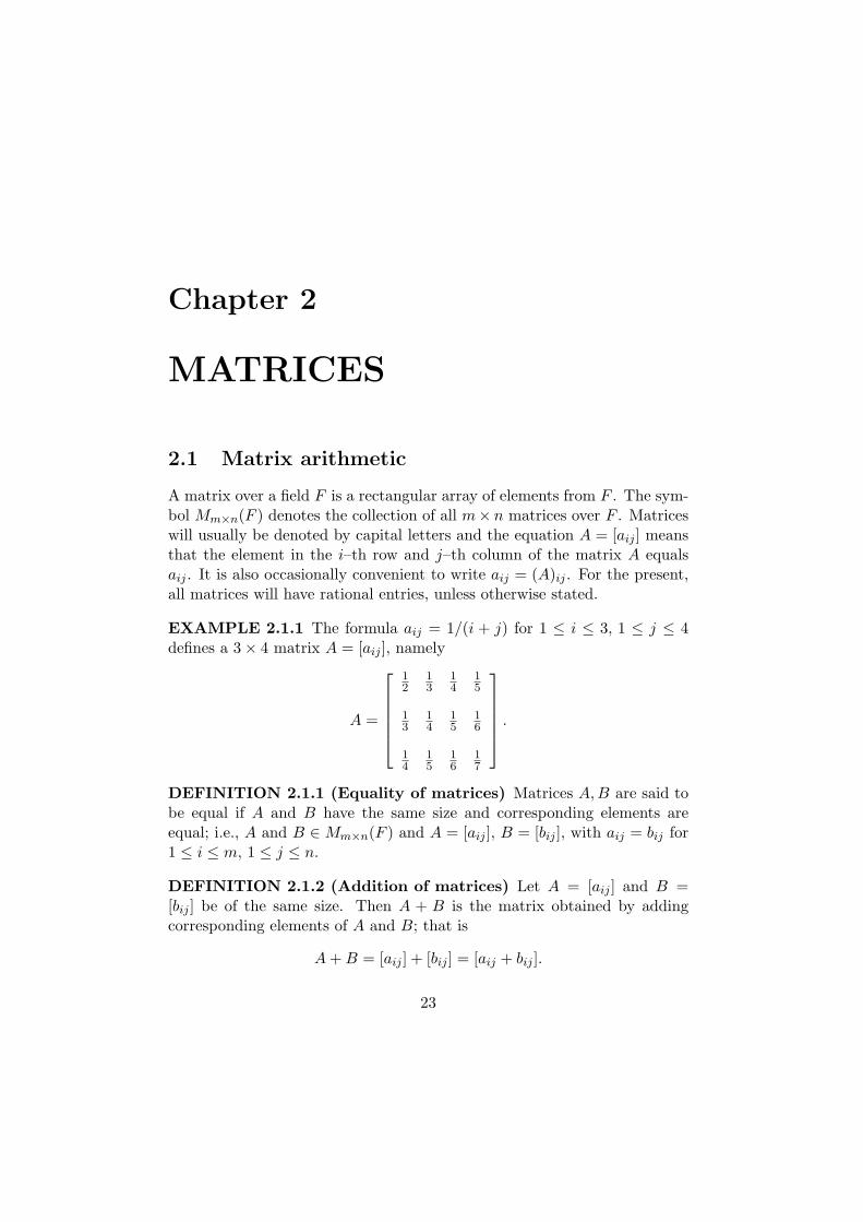
34 CHAPTER 2. MATRICES
C =
−3 −12 14 3
, D =
[
4 −12 0
]
.
Which of the following matrices are defined? Compute those matriceswhich are defined.
A + B, A + C, AB, BA, CD, DC, D2.
[Answers: A + C, BA, CD, D2;
0 −11 35 4
,
0 12−4 2−10 5
,
−14 310 −222 −4
,
[
14 −48 −2
]
.]
2. Let A =
[
−1 0 10 1 1
]
. Show that if B is a 3 × 2 such that AB = I2,
then
B =
a b−a − 1 1 − ba + 1 b
for suitable numbers a and b. Use the associative law to show that(BA)2B = B.
3. If A =
[
a bc d
]
, prove that A2 − (a + d)A + (ad − bc)I2 = 0.
4. If A =
[
4 −31 0
]
, use the fact A2 = 4A − 3I2 and mathematical
induction, to prove that
An =(3n − 1)
2A +
3 − 3n
2I2 if n ≥ 1.
5. A sequence of numbers x1, x2, . . . , xn, . . . satisfies the recurrence rela-tion xn+1 = axn +bxn−1 for n ≥ 1, where a and b are constants. Provethat
[
xn+1
xn
]
= A
[
xn
xn−1
]
,

2.4. PROBLEMS 35
where A =
[
a b1 0
]
and hence express
[
xn+1
xn
]
in terms of
[
x1
x0
]
.
If a = 4 and b = −3, use the previous question to find a formula forxn in terms of x1 and x0.
[Answer:
xn =3n − 1
2x1 +
3 − 3n
2x0.]
6. Let A =
[
2a −a2
1 0
]
.
(a) Prove that
An =
[
(n + 1)an −nan+1
nan−1 (1 − n)an
]
if n ≥ 1.
(b) A sequence x0, x1, . . . , xn, . . . satisfies xn+1 = 2axn − a2xn−1 forn ≥ 1. Use part (a) and the previous question to prove thatxn = nan−1x1 + (1 − n)anx0 for n ≥ 1.
7. Let A =
[
a bc d
]
and suppose that λ1 and λ2 are the roots of the
quadratic polynomial x2−(a+d)x+ad−bc. (λ1 and λ2 may be equal.)
Let kn be defined by k0 = 0, k1 = 1 and for n ≥ 2
kn =
n∑
i=1
λn−i1 λi−1
2 .
Prove thatkn+1 = (λ1 + λ2)kn − λ1λ2kn−1,
if n ≥ 1. Also prove that
kn =
{
(λn1 − λn
2 )/(λ1 − λ2) if λ1 6= λ2,
nλn−11 if λ1 = λ2.
Use mathematical induction to prove that if n ≥ 1,
An = knA − λ1λ2kn−1I2,
[Hint: Use the equation A2 = (a + d)A − (ad − bc)I2.]

36 CHAPTER 2. MATRICES
8. Use Question 7 to prove that if A =
[
1 22 1
]
, then
An =3n
2
[
1 11 1
]
+(−1)n−1
2
[
−1 11 −1
]
if n ≥ 1.
9. The Fibonacci numbers are defined by the equations F0 = 0, F1 = 1and Fn+1 = Fn + Fn−1 if n ≥ 1. Prove that
Fn =1√5
((
1 +√
5
2
)n
−(
1 −√
5
2
)n)
if n ≥ 0.
10. Let r > 1 be an integer. Let a and b be arbitrary positive integers.Sequences xn and yn of positive integers are defined in terms of a andb by the recurrence relations
xn+1 = xn + ryn
yn+1 = xn + yn,
for n ≥ 0, where x0 = a and y0 = b.
Use Question 7 to prove that
xn
yn→
√r as n → ∞.
2.5 Non–singular matrices
DEFINITION 2.5.1 (Non–singular matrix) A matrix A ∈ Mn×n(F )is called non–singular or invertible if there exists a matrix B ∈ Mn×n(F )such that
AB = In = BA.
Any matrix B with the above property is called an inverse of A. If A doesnot have an inverse, A is called singular.
THEOREM 2.5.1 (Inverses are unique) If A has inverses B and C,then B = C.

2.5. NON–SINGULAR MATRICES 37
Proof. Let B and C be inverses of A. Then AB = In = BA and AC =In = CA. Then B(AC) = BIn = B and (BA)C = InC = C. Hence becauseB(AC) = (BA)C, we deduce that B = C.
REMARK 2.5.1 If A has an inverse, it is denoted by A−1. So
AA−1 = In = A−1A.
Also if A is non–singular, it follows that A−1 is also non–singular and
(A−1)−1 = A.
THEOREM 2.5.2 If A and B are non–singular matrices of the same size,then so is AB. Moreover
(AB)−1 = B−1A−1.
Proof.
(AB)(B−1A−1) = A(BB−1)A−1 = AInA−1 = AA−1 = In.
Similarly(B−1A−1)(AB) = In.
REMARK 2.5.2 The above result generalizes to a product of m non–singular matrices: If A1, . . . , Am are non–singular n × n matrices, then theproduct A1 . . . Am is also non–singular. Moreover
(A1 . . . Am)−1 = A−1m . . . A−1
1 .
(Thus the inverse of the product equals the product of the inverses in the
reverse order.)
EXAMPLE 2.5.1 If A and B are n × n matrices satisfying A2 = B2 =(AB)2 = In, prove that AB = BA.
Solution. Assume A2 = B2 = (AB)2 = In. Then A, B, AB are non–singular and A−1 = A, B−1 = B, (AB)−1 = AB.
But (AB)−1 = B−1A−1 and hence AB = BA.
EXAMPLE 2.5.2 A =
[
1 24 8
]
is singular. For suppose B =
[
a bc d
]
is an inverse of A. Then the equation AB = I2 gives[
1 24 8
] [
a bc d
]
=
[
1 00 1
]

38 CHAPTER 2. MATRICES
and equating the corresponding elements of column 1 of both sides gives thesystem
a + 2c = 1
4a + 8c = 0
which is clearly inconsistent.
THEOREM 2.5.3 Let A =
[
a bc d
]
and ∆ = ad − bc 6= 0. Then A is
non–singular. Also
A−1 = ∆−1
[
d −b−c a
]
.
REMARK 2.5.3 The expression ad − bc is called the determinant of A
and is denoted by the symbols detA or
∣
∣
∣
∣
a bc d
∣
∣
∣
∣
.
Proof. Verify that the matrix B = ∆−1
[
d −b−c a
]
satisfies the equation
AB = I2 = BA.
EXAMPLE 2.5.3 Let
A =
0 1 00 0 15 0 0
.
Verify that A3 = 5I3, deduce that A is non–singular and find A−1.
Solution. After verifying that A3 = 5I3, we notice that
A
(
1
5A2
)
= I3 =
(
1
5A2
)
A.
Hence A is non–singular and A−1 = 15A2.
THEOREM 2.5.4 If the coefficient matrix A of a system of n equationsin n unknowns is non–singular, then the system AX = B has the uniquesolution X = A−1B.
Proof. Assume that A−1 exists.

2.5. NON–SINGULAR MATRICES 39
1. (Uniqueness.) Assume that AX = B. Then
(A−1A)X = A−1B,
InX = A−1B,
X = A−1B.
2. (Existence.) Let X = A−1B. Then
AX = A(A−1B) = (AA−1)B = InB = B.
THEOREM 2.5.5 (Cramer’s rule for 2 equations in 2 unknowns)The system
ax + by = e
cx + dy = f
has a unique solution if ∆ =
∣
∣
∣
∣
a bc d
∣
∣
∣
∣
6= 0, namely
x =∆1
∆, y =
∆2
∆,
where
∆1 =
∣
∣
∣
∣
e bf d
∣
∣
∣
∣
and ∆2 =
∣
∣
∣
∣
a ec f
∣
∣
∣
∣
.
Proof. Suppose ∆ 6= 0. Then A =
[
a bc d
]
has inverse
A−1 = ∆−1
[
d −b−c a
]
and we know that the system
A
[
xy
]
=
[
ef
]
has the unique solution[
xy
]
= A−1
[
ef
]
=1
∆
[
d −b−c a
] [
ef
]
=1
∆
[
de − bf−ce + af
]
=1
∆
[
∆1
∆2
]
=
[
∆1/∆∆2/∆
]
.
Hence x = ∆1/∆, y = ∆2/∆.

40 CHAPTER 2. MATRICES
COROLLARY 2.5.1 The homogeneous system
ax + by = 0
cx + dy = 0
has only the trivial solution if ∆ =
∣
∣
∣
∣
a bc d
∣
∣
∣
∣
6= 0.
EXAMPLE 2.5.4 The system
7x + 8y = 100
2x − 9y = 10
has the unique solution x = ∆1/∆, y = ∆2/∆, where
∆=
˛
˛
˛
˛
˛
˛
7 82 −9
˛
˛
˛
˛
˛
˛
=−79, ∆1=
˛
˛
˛
˛
˛
˛
100 810 −9
˛
˛
˛
˛
˛
˛
=−980, ∆2=
˛
˛
˛
˛
˛
˛
7 1002 10
˛
˛
˛
˛
˛
˛
=−130.
So x = 98079 and y = 130
79 .
THEOREM 2.5.6 Let A be a square matrix. If A is non–singular, thehomogeneous system AX = 0 has only the trivial solution. Equivalently,if the homogenous system AX = 0 has a non–trivial solution, then A issingular.
Proof. If A is non–singular and AX = 0, then X = A−10 = 0.
REMARK 2.5.4 If A∗1, . . . , A∗n denote the columns of A, then the equa-tion
AX = x1A∗1 + . . . + xnA∗n
holds. Consequently theorem 2.5.6 tells us that if there exist x1, . . . , xn, not
all zero, such that
x1A∗1 + . . . + xnA∗n = 0,
that is, if the columns of A are linearly dependent, then A is singular. Anequivalent way of saying that the columns of A are linearly dependent is thatone of the columns of A is expressible as a sum of certain scalar multiplesof the remaining columns of A; that is one column is a linear combination
of the remaining columns.

2.5. NON–SINGULAR MATRICES 41
EXAMPLE 2.5.5
A =
1 2 31 0 13 4 7
is singular. For it can be verified that A has reduced row–echelon form
1 0 10 1 10 0 0
and consequently AX = 0 has a non–trivial solution x = −1, y = −1, z = 1.
REMARK 2.5.5 More generally, if A is row–equivalent to a matrix con-taining a zero row, then A is singular. For then the homogeneous systemAX = 0 has a non–trivial solution.
An important class of non–singular matrices is that of the elementary
row matrices.
DEFINITION 2.5.2 (Elementary row matrices) To each of the threetypes of elementary row operation, there corresponds an elementary row
matrix, denoted by Eij , Ei(t), Eij(t):
1. Eij , (i 6= j) is obtained from the identity matrix In by interchangingrows i and j.
2. Ei(t), (t 6= 0) is obtained by multiplying the i–th row of In by t.
3. Eij(t), (i 6= j) is obtained from In by adding t times the j–th row ofIn to the i–th row.
EXAMPLE 2.5.6 (n = 3.)
E23 =
1 0 00 0 10 1 0
, E2(−1) =
1 0 00 −1 00 0 1
, E23(−1) =
1 0 00 1 −10 0 1
.
The elementary row matrices have the following distinguishing property:
THEOREM 2.5.7 If a matrix A is pre–multiplied by an elementary rowmatrix, the resulting matrix is the one obtained by performing the corre-sponding elementary row–operation on A.

42 CHAPTER 2. MATRICES
EXAMPLE 2.5.7
E23
a bc de f
=
1 0 00 0 10 1 0
a bc de f
=
a be fc d
.
COROLLARY 2.5.2 Elementary row–matrices are non–singular. Indeed
1. E−1ij = Eij ;
2. E−1i (t) = Ei(t
−1);
3. (Eij(t))−1 = Eij(−t).
Proof. Taking A = In in the above theorem, we deduce the followingequations:
EijEij = In
Ei(t)Ei(t−1) = In = Ei(t
−1)Ei(t) if t 6= 0
Eij(t)Eij(−t) = In = Eij(−t)Eij(t).
EXAMPLE 2.5.8 Find the 3 × 3 matrix A = E3(5)E23(2)E12 explicitly.Also find A−1.
Solution.
A = E3(5)E23(2)
0 1 01 0 00 0 1
= E3(5)
0 1 01 0 20 0 1
=
0 1 01 0 20 0 5
.
To find A−1, we have
A−1 = (E3(5)E23(2)E12)−1
= E−112 (E23(2))−1 (E3(5))−1
= E12E23(−2)E3(5−1)
= E12E23(−2)
1 0 00 1 00 0 1
5
= E12
1 0 00 1 −2
50 0 1
5
=
0 1 −25
1 0 00 0 1
5
.
2.5. NON–SINGULAR MATRICES 43
REMARK 2.5.6 Recall that A and B are row–equivalent if B is obtainedfrom A by a sequence of elementary row operations. If E1, . . . , Er are therespective corresponding elementary row matrices, then
B = Er (. . . (E2(E1A)) . . .) = (Er . . . E1)A = PA,
where P = Er . . . E1 is non–singular. Conversely if B = PA, where P isnon–singular, then A is row–equivalent to B. For as we shall now see, P isin fact a product of elementary row matrices.
THEOREM 2.5.8 Let A be non–singular n × n matrix. Then
(i) A is row–equivalent to In,
(ii) A is a product of elementary row matrices.
Proof. Assume that A is non–singular and let B be the reduced row–echelonform of A. Then B has no zero rows, for otherwise the equation AX = 0would have a non–trivial solution. Consequently B = In.
It follows that there exist elementary row matrices E1, . . . , Er such thatEr (. . . (E1A) . . .) = B = In and hence A = E−1
1 . . . E−1r , a product of
elementary row matrices.
THEOREM 2.5.9 Let A be n × n and suppose that A is row–equivalentto In. Then A is non–singular and A−1 can be found by performing thesame sequence of elementary row operations on In as were used to convertA to In.
Proof. Suppose that Er . . . E1A = In. In other words BA = In, whereB = Er . . . E1 is non–singular. Then B−1(BA) = B−1In and so A = B−1,which is non–singular.
Also A−1 =(
B−1)−1
= B = Er ((. . . (E1In) . . .), which shows that A−1
is obtained from In by performing the same sequence of elementary rowoperations as were used to convert A to In.
REMARK 2.5.7 It follows from theorem 2.5.9 that if A is singular, thenA is row–equivalent to a matrix whose last row is zero.
EXAMPLE 2.5.9 Show that A =
[
1 21 1
]
is non–singular, find A−1 and
express A as a product of elementary row matrices.

44 CHAPTER 2. MATRICES
Solution. We form the partitioned matrix [A|I2] which consists of A followedby I2. Then any sequence of elementary row operations which reduces A toI2 will reduce I2 to A−1. Here
[A|I2] =
[
1 2 1 01 1 0 1
]
R2 → R2 − R1
[
1 2 1 00 −1 −1 1
]
R2 → (−1)R2
[
1 2 1 00 1 1 −1
]
R1 → R1 − 2R2
[
1 0 −1 20 1 1 −1
]
.
Hence A is row–equivalent to I2 and A is non–singular. Also
A−1 =
[
−1 21 −1
]
.
We also observe that
E12(−2)E2(−1)E21(−1)A = I2.
Hence
A−1 = E12(−2)E2(−1)E21(−1)
A = E21(1)E2(−1)E12(2).
The next result is the converse of Theorem 2.5.6 and is useful for provingthe non–singularity of certain types of matrices.
THEOREM 2.5.10 Let A be an n × n matrix with the property thatthe homogeneous system AX = 0 has only the trivial solution. Then A isnon–singular. Equivalently, if A is singular, then the homogeneous systemAX = 0 has a non–trivial solution.
Proof. If A is n × n and the homogeneous system AX = 0 has only thetrivial solution, then it follows that the reduced row–echelon form B of Acannot have zero rows and must therefore be In. Hence A is non–singular.
COROLLARY 2.5.3 Suppose that A and B are n × n and AB = In.Then BA = In.

2.5. NON–SINGULAR MATRICES 45
Proof. Let AB = In, where A and B are n × n. We first show that Bis non–singular. Assume BX = 0. Then A(BX) = A0 = 0, so (AB)X =0, InX = 0 and hence X = 0.
Then from AB = In we deduce (AB)B−1 = InB−1 and hence A = B−1.The equation BB−1 = In then gives BA = In.
Before we give the next example of the above criterion for non-singularity,we introduce an important matrix operation.
DEFINITION 2.5.3 (The transpose of a matrix) Let A be an m×nmatrix. Then At, the transpose of A, is the matrix obtained by interchangingthe rows and columns of A. In other words if A = [aij ], then
(
At)
ji= aij .
Consequently At is n × m.
The transpose operation has the following properties:
1.(
At)t
= A;
2. (A ± B)t = At ± Bt if A and B are m × n;
3. (sA)t = sAt if s is a scalar;
4. (AB)t = BtAt if A is m × n and B is n × p;
5. If A is non–singular, then At is also non–singular and
(
At)−1
=(
A−1)t
;
6. XtX = x21 + . . . + x2
n if X = [x1, . . . , xn]t is a column vector.
We prove only the fourth property. First check that both (AB)t and BtAt
have the same size (p × m). Moreover, corresponding elements of bothmatrices are equal. For if A = [aij ] and B = [bjk], we have
(
(AB)t)
ki= (AB)ik
=n
∑
j=1
aijbjk
=n
∑
j=1
(
Bt)
kj
(
At)
ji
=(
BtAt)
ki.
There are two important classes of matrices that can be defined conciselyin terms of the transpose operation.

46 CHAPTER 2. MATRICES
DEFINITION 2.5.4 (Symmetric matrix) A matrix A is symmetric ifAt = A. In other words A is square (n × n say) and aji = aij for all1 ≤ i ≤ n, 1 ≤ j ≤ n. Hence
A =
[
a bb c
]
is a general 2 × 2 symmetric matrix.
DEFINITION 2.5.5 (Skew–symmetric matrix) A matrix A is calledskew–symmetric if At = −A. In other words A is square (n × n say) andaji = −aij for all 1 ≤ i ≤ n, 1 ≤ j ≤ n.
REMARK 2.5.8 Taking i = j in the definition of skew–symmetric matrixgives aii = −aii and so aii = 0. Hence
A =
[
0 b−b 0
]
is a general 2 × 2 skew–symmetric matrix.
We can now state a second application of the above criterion for non–singularity.
COROLLARY 2.5.4 Let B be an n × n skew–symmetric matrix. ThenA = In − B is non–singular.
Proof. Let A = In − B, where Bt = −B. By Theorem 2.5.10 it suffices toshow that AX = 0 implies X = 0.
We have (In − B)X = 0, so X = BX. Hence XtX = XtBX.
Taking transposes of both sides gives
(XtBX)t = (XtX)t
XtBt(Xt)t = Xt(Xt)t
Xt(−B)X = XtX
−XtBX = XtX = XtBX.
Hence XtX = −XtX and XtX = 0. But if X = [x1, . . . , xn]t, then XtX =x2
1 + . . . + x2n = 0 and hence x1 = 0, . . . , xn = 0.

2.6. LEAST SQUARES SOLUTION OF EQUATIONS 47
2.6 Least squares solution of equations
Suppose AX = B represents a system of linear equations with real coeffi-cients which may be inconsistent, because of the possibility of experimentalerrors in determining A or B. For example, the system
x = 1
y = 2
x + y = 3.001
is inconsistent.It can be proved that the associated system AtAX = AtB is always
consistent and that any solution of this system minimizes the sum r21 + . . .+
r2m, where r1, . . . , rm (the residuals) are defined by
ri = ai1x1 + . . . + ainxn − bi,
for i = 1, . . . , m. The equations represented by AtAX = AtB are called thenormal equations corresponding to the system AX = B and any solutionof the system of normal equations is called a least squares solution of theoriginal system.
EXAMPLE 2.6.1 Find a least squares solution of the above inconsistentsystem.
Solution. Here A =
1 00 11 1
, X =
[
xy
]
, B =
12
3.001
.
Then AtA =
[
1 0 10 1 1
]
1 00 11 1
=
[
2 11 2
]
.
Also AtB =
[
1 0 10 1 1
]
12
3.001
=
[
4.0015.001
]
.
So the normal equations are
2x + y = 4.001
x + 2y = 5.001
which have the unique solution
x =3.001
3, y =
6.001
3.

48 CHAPTER 2. MATRICES
EXAMPLE 2.6.2 Points (x1, y1), . . . , (xn, yn) are experimentally deter-mined and should lie on a line y = mx + c. Find a least squares solution tothe problem.
Solution. The points have to satisfy
mx1 + c = y1
...
mxn + c = yn,
or Ax = B, where
A =
x1 1...
...xn 1
, X =
[
mc
]
, B =
y1...
yn
.
The normal equations are given by (AtA)X = AtB. Here
AtA =
[
x1 . . . xn
1 . . . 1
]
x1 1...
...xn 1
=
[
x21 + . . . + x2
n x1 + . . . + xn
x1 + . . . + xn n
]
Also
AtB =
[
x1 . . . xn
1 . . . 1
]
y1...
yn
=
[
x1y1 + . . . + xnyn
y1 + . . . + yn
]
.
It is not difficult to prove that
∆ = det (AtA) =∑
1≤i<j≤n
(xi − xj)2,
which is positive unless x1 = . . . = xn. Hence if not all of x1, . . . , xn areequal, AtA is non–singular and the normal equations have a unique solution.This can be shown to be
m =1
∆
∑
1≤i<j≤n
(xi − xj)(yi − yj), c =1
∆
∑
1≤i<j≤n
(xiyj − xjyi)(xi − xj).
REMARK 2.6.1 The matrix AtA is symmetric.

2.7. PROBLEMS 49
2.7 PROBLEMS
1. Let A =
[
1 4−3 1
]
. Prove that A is non–singular, find A−1 and
express A as a product of elementary row matrices.
[Answer: A−1 =
[
113 − 4
13313
113
]
,
A = E21(−3)E2(13)E12(4) is one such decomposition.]
2. A square matrix D = [dij ] is called diagonal if dij = 0 for i 6= j. (Thatis the off–diagonal elements are zero.) Prove that pre–multiplicationof a matrix A by a diagonal matrix D results in matrix DA whoserows are the rows of A multiplied by the respective diagonal elementsof D. State and prove a similar result for post–multiplication by adiagonal matrix.
Let diag (a1, . . . , an) denote the diagonal matrix whose diagonal ele-ments dii are a1, . . . , an, respectively. Show that
diag (a1, . . . , an)diag (b1, . . . , bn) = diag (a1b1, . . . , anbn)
and deduce that if a1 . . . an 6= 0, then diag (a1, . . . , an) is non–singularand
(diag (a1, . . . , an))−1 = diag (a−11 , . . . , a−1
n ).
Also prove that diag (a1, . . . , an) is singular if ai = 0 for some i.
3. Let A =
0 0 21 2 63 7 9
. Prove that A is non–singular, find A−1 and
express A as a product of elementary row matrices.
[Answers: A−1 =
−12 7 −292 −3 112 0 0
,
A = E12E31(3)E23E3(2)E12(2)E13(24)E23(−9) is one such decompo-sition.]

50 CHAPTER 2. MATRICES
4. Find the rational number k for which the matrix A =
1 2 k3 −1 15 3 −5
is singular. [Answer: k = −3.]
5. Prove that A =
[
1 2−2 −4
]
is singular and find a non–singular matrix
P such that PA has last row zero.
6. If A =
[
1 4−3 1
]
, verify that A2 − 2A + 13I2 = 0 and deduce that
A−1 = − 113(A − 2I2).
7. Let A =
1 1 −10 0 12 1 2
.
(i) Verify that A3 = 3A2 − 3A + I3.
(ii) Express A4 in terms of A2, A and I3 and hence calculate A4
explicitly.
(iii) Use (i) to prove that A is non–singular and find A−1 explicitly.
[Answers: (ii) A4 = 6A2 − 8A + 3I3 =
−11 −8 −412 9 420 16 5
;
(iii) A−1 = A2 − 3A + 3I3 =
−1 −3 12 4 −10 1 0
.]
8. (i) Let B be an n×n matrix such that B3 = 0. If A = In−B, provethat A is non–singular and A−1 = In + B + B2.
Show that the system of linear equations AX = b has the solution
X = b + Bb + B2b.
(ii) If B =
0 r s0 0 t0 0 0
, verify that B3 = 0 and use (i) to determine
(I3 − B)−1 explicitly.

2.7. PROBLEMS 51
[Answer:
1 r s + rt0 1 t0 0 1
.]
9. Let A be n × n.
(i) If A2 = 0, prove that A is singular.
(ii) If A2 = A and A 6= In, prove that A is singular.
10. Use Question 7 to solve the system of equations
x + y − z = a
z = b
2x + y + 2z = c
where a, b, c are given rationals. Check your answer using the Gauss–Jordan algorithm.
[Answer: x = −a − 3b + c, y = 2a + 4b − c, z = b.]
11. Determine explicitly the following products of 3 × 3 elementary rowmatrices.
(i) E12E23 (ii) E1(5)E12 (iii) E12(3)E21(−3) (iv) (E1(100))−1
(v) E−112 (vi) (E12(7))−1 (vii) (E12(7)E31(1))−1.
[Answers: (i)
2
4
0 0 11 0 00 1 0
3
5 (ii)
2
4
0 5 01 0 00 0 1
3
5 (iii)
2
4
−8 3 0−3 1 0
0 0 1
3
5
(iv)
2
4
1/100 0 00 1 00 0 1
3
5 (v)
2
4
0 1 01 0 00 0 1
3
5 (vi)
2
4
1 −7 00 1 00 0 1
3
5 (vii)
2
4
1 −7 00 1 0
−1 7 1
3
5.]
12. Let A be the following product of 4 × 4 elementary row matrices:
A = E3(2)E14E42(3).
Find A and A−1 explicitly.
[Answers: A =
2
6
6
4
0 3 0 10 1 0 00 0 2 01 0 0 0
3
7
7
5
, A−1 =
2
6
6
4
0 0 0 10 1 0 00 0 1/2 01 −3 0 0
3
7
7
5
.]

52 CHAPTER 2. MATRICES
13. Determine which of the following matrices over Z2 are non–singularand find the inverse, where possible.
(a)
2
6
6
4
1 1 0 10 0 1 11 1 1 11 0 0 1
3
7
7
5
(b)
2
6
6
4
1 1 0 10 1 1 11 0 1 01 1 0 1
3
7
7
5
. [Answer: (a)
2
6
6
4
1 1 1 11 0 0 11 0 1 01 1 1 0
3
7
7
5
.]
14. Determine which of the following matrices are non–singular and findthe inverse, where possible.
(a)
2
4
1 1 1−1 1 0
2 0 0
3
5 (b)
2
4
2 2 41 0 10 1 0
3
5 (c)
2
4
4 6 −30 0 70 0 5
3
5
(d)
2
4
2 0 00 −5 00 0 7
3
5 (e)
2
6
6
4
1 2 4 60 1 2 00 0 1 20 0 0 2
3
7
7
5
(f)
2
4
1 2 34 5 65 7 9
3
5.
[Answers: (a)
2
4
0 0 1/20 1 1/21 −1 −1
3
5 (b)
2
4
−1/2 2 10 0 1
1/2 −1 −1
3
5 (d)
2
4
1/2 0 00 −1/5 00 0 1/7
3
5
(e)
2
6
6
4
1 −2 0 −30 1 −2 20 0 1 −10 0 0 1/2
3
7
7
5
.]
15. Let A be a non–singular n × n matrix. Prove that At is non–singularand that (At)−1 = (A−1)t.
16. Prove that A =
[
a bc d
]
has no inverse if ad − bc = 0.
[Hint: Use the equation A2 − (a + d)A + (ad − bc)I2 = 0.]
17. Prove that the real matrix A =
2
4
1 a b−a 1 c−b −c 1
3
5 is non–singular by prov-
ing that A is row–equivalent to I3.
18. If P−1AP = B, prove that P−1AnP = Bn for n ≥ 1.

2.7. PROBLEMS 53
19. Let A =
[
2/3 1/41/3 3/4
]
, P =
[
1 3−1 4
]
. Verify that P−1AP =[
5/12 00 1
]
and deduce that
An =1
7
[
3 34 4
]
+1
7
(
5
12
)n [
4 −3−4 3
]
.
20. Let A =
[
a bc d
]
be a Markov matrix; that is a matrix whose elements
are non–negative and satisfy a+c = 1 = b+d. Also let P =
[
b 1c −1
]
.
Prove that if A 6= I2 then
(i) P is non–singular and P−1AP =
[
1 00 a + d − 1
]
,
(ii) An → 1
b + c
[
b bc c
]
as n → ∞, if A 6=[
0 11 0
]
.
21. If X =
1 23 45 6
and Y =
−134
, find XXt, XtX, Y Y t, Y tY .
[Answers:
5 11 1711 25 3917 39 61
,
[
35 4444 56
]
,
1 −3 −4−3 9 12−4 12 16
, 26.]
22. Prove that the system of linear equations
x + 2y = 4x + y = 5
3x + 5y = 12
is inconsistent and find a least squares solution of the system.
[Answer: x = 6, y = −7/6.]
23. The points (0, 0), (1, 0), (2, −1), (3, 4), (4, 8) are required to lie on aparabola y = a + bx + cx2. Find a least squares solution for a, b, c.Also prove that no parabola passes through these points.
[Answer: a = 15 , b = −2, c = 1.]

54 CHAPTER 2. MATRICES
24. If A is a symmetric n×n real matrix and B is n×m, prove that BtABis a symmetric m × m matrix.
25. If A is m × n and B is n × m, prove that AB is singular if m > n.
26. Let A and B be n × n. If A or B is singular, prove that AB is alsosingular.


![Untitled-1 [] · 2019. 4. 17. · inequalities, permutations and combinations, binomial theorem, number theory. Vector spaces and subspaces, linear dependence, matrices: their rank](https://img.pdfslide.us/doc/110x75/600b555f1bfe3420db70b400/untitled-1-2019-4-17-inequalities-permutations-and-combinations-binomial.jpg)