Embed Size (px)
Citation preview
Theory of Large Dimensional Random Matrices for Engineers
(Part I)
Antonia M. TulinoUniversità degli Studi di Napoli, "Federico II"
The 9th International Symposium on Spread Spectrum Techniques and Applications, Manaus, Amazon, Brazil,
August 28-31, 2006

Outline
• A brief historical tour of the main results in random matrix theory.
Overview some of the main transforms.
Fundamental limits of wireless communications: basic channels.
For these basic channels, we analyze some performance measures ofengineering interest.
Stieltjes transform, and its role in understanding eigenvalues of randommatrices
Limit theorems of three classes of random matrices
Proof of one of the theorems
1

Outline
• A brief historical tour of the main results in random matrix theory.
• Overview some of the main transforms.
Fundamental limits of wireless communications: basic channels.
For these basic channels, we analyze some performance measures ofengineering interest.
Stieltjes transform, and its role in understanding eigenvalues of randommatrices
Limit theorems of three classes of random matrices
Proof of one of the theorems
2
Outline
• A brief historical tour of the main results in random matrix theory.
• Overview some of the main transforms.
• Fundamental limits of wireless communications: basic channels.
For these basic channels, we analyze some performance measures ofengineering interest.
Stieltjes transform, and its role in understanding eigenvalues of randommatrices
Limit theorems of three classes of random matrices
Proof of one of the theorems
3

Outline
• A brief historical tour of the main results in random matrix theory.
• Overview some of the main transforms.
• Fundamental limits of wireless communications: basic channels.
• Performance measures of engineering interest (Signal Processing /Information Theory).
Stieltjes transform, and its role in understanding eigenvalues of randommatrices
Limit theorems of three classes of random matrices
Proof of one of the theorems
4

Outline
• A brief historical tour of the main results in random matrix theory.
• Overview some of the main transforms.
• Fundamental limits of wireless communications: basic channels.
• Performance measures of engineering interest (Signal Processing /Information Theory).
• Stieltjes transform, and its role in understanding eigenvalues of randommatrices (Part II)
Limit theorems of three classes of random matrices
Proof of one of the theorems
5

Outline
• A brief historical tour of the main results in random matrix theory.
• Overview some of the main transforms.
• Fundamental limits of wireless communications: basic channels.
• Performance measures of engineering interest (Signal Processing /Information Theory).
• Stieltjes transform, and its role in understanding eigenvalues of randommatrices (Part II)
• Limit theorems of three classes of random matrices (Part II)
Proof of one of the theorems
6
Outline
• A brief historical tour of the main results in random matrix theory.
• Overview some of the main transforms.
• Fundamental limits of wireless communications: basic channels.
• Performance measures of engineering interest (Signal Processing /Information Theory).
• Stieltjes transform, and its role in understanding eigenvalues of randommatrices (Part II)
• Limit theorems of three classes of random matrices (Part II)
• Proof of one of the theorems (Part II)
7
Introduction
• Today random matrices find applications in fields as diverse as theRiemann hypothesis, stochastic differential equations, statistical physics,chaotic systems, numerical linear algebra, neural networks, etc.
• Random matrices are also finding an increasing number of applicationsin the context of information theory and signal processing.
8

Random Matrices & Information Theory
• The applications in information theory include, among others:
X Wireless communications channelsX Learning and neural networksX Capacity of ad hoc networksX Speed of convergence of iterative algorithms for multiuser detectionX Direction of arrival estimation in sensor arrays
• Earliest applications to wireless communication : works of Foschini andTelatar, in the mid-90s, on characterizing the capacity of multi-antennachannels.
A. M. Tulino and S. Verdu“Random Matrices and Wireless Communications,”
Foundations and Trends in Communications and Information Theory,vol. 1, no. 1, June 2004.
9
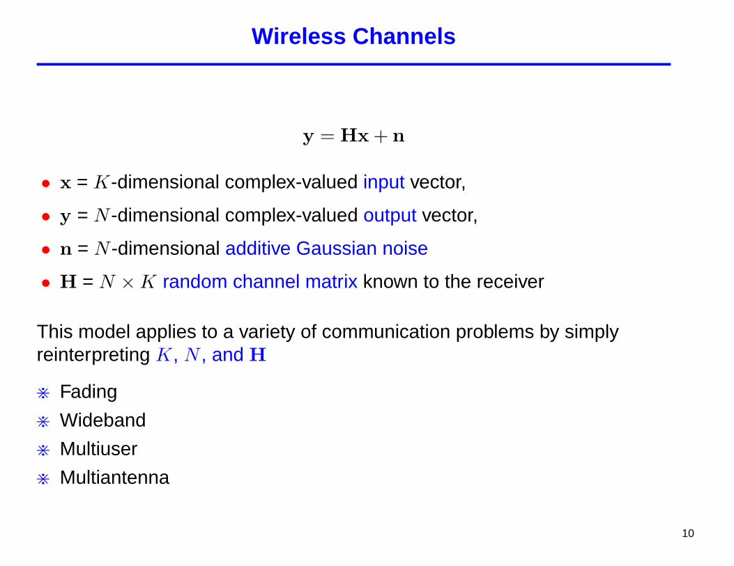
Wireless Channels
y = Hx + n
• x = K-dimensional complex-valued input vector,
• y = N -dimensional complex-valued output vector,
• n = N -dimensional additive Gaussian noise
• H = N ×K random channel matrix known to the receiver
This model applies to a variety of communication problems by simplyreinterpreting K, N , and H
> Fading
> Wideband
> Multiuser
> Multiantenna
10

Multi-Antenna channels
K
N
y = Hx + n
• K and N number of transmit and receive antennas
• H = propagation matrix: N ×K complex matrix whose entries representthe gains between each transmit and each receive antenna.
11

Multi-Antenna channels
K
N
N Prototype picture courtesy ofBell Labs (Lucent Technologies)
y = Hx + n
• K and N number of transmit and receive antennas
• H = propagation matrix: N ×K complex matrix whose entries representthe gains between each transmit and each receive antenna.
12
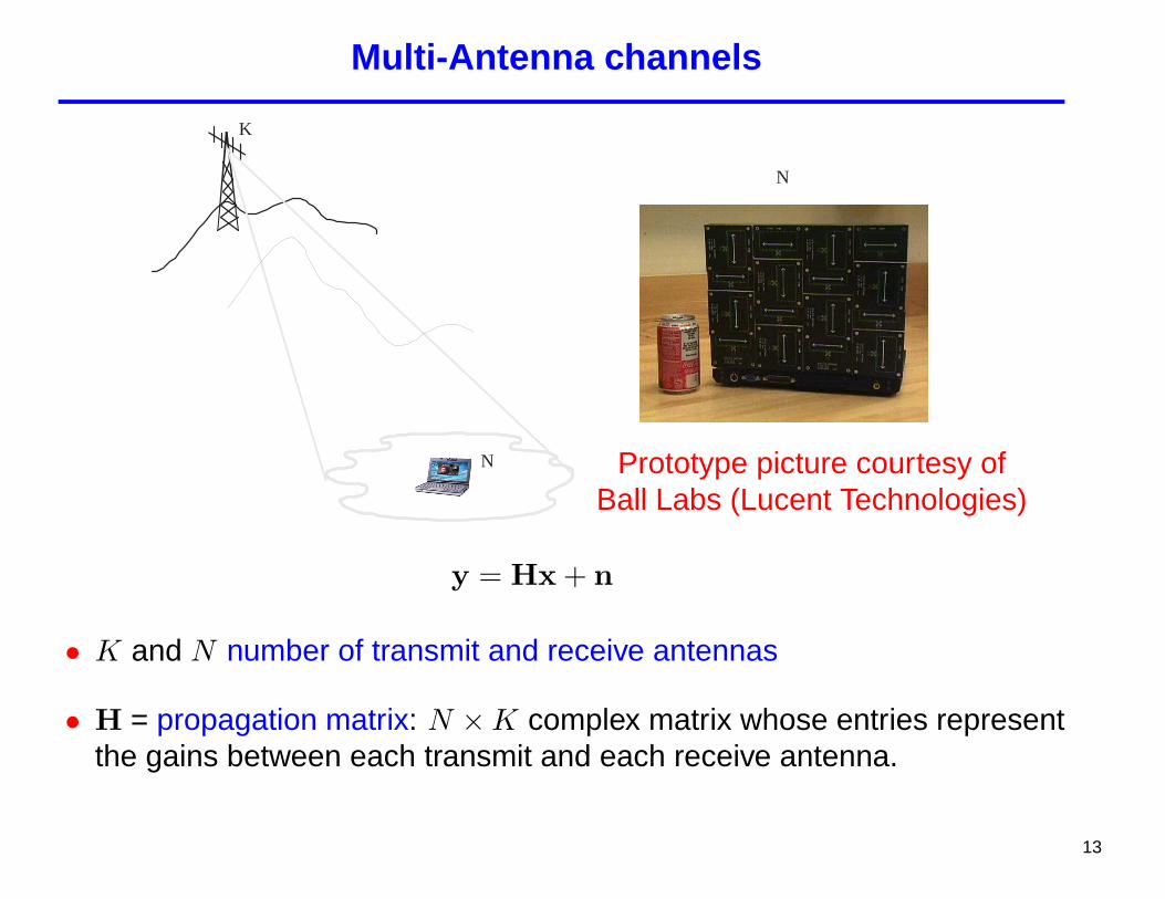
Multi-Antenna channels
K
N
N Prototype picture courtesy ofBall Labs (Lucent Technologies)
y = Hx + n
• K and N number of transmit and receive antennas
• H = propagation matrix: N ×K complex matrix whose entries representthe gains between each transmit and each receive antenna.
13

CDMA (Code-Division Multiple Access) Channel
Signal space with N dimensions.N= “spreading gain” = proportional to Bandwidth
Each user assigned a “signature vector” known at the receiver
User 2
User 1 c h a n n e l
c h a n n e l c h a n n e l
. . .
. . .
. . .
Interface
Interface
x 2
x 1
> DS-CDMA (Direct sequence CDMA) used in many current cellularsystems (IS-95, cdma2000, UMTS).
> MC-CDMA (Multi-Carrier CDMA) being considered for 4G (FourthGeneration) wireless.
14

DS-CDMA Flat-faded Channel
User 2
User 1 A 1 1 s 1
A 2 2 s 2
A k k s k
. . .
. . . . . .
Interface
Interface
Front End
y=Hx + n
x 2
x 1
y = H︸︷︷︸SA
x + n= SAx + n
• K= number of users; N= processing gain.
• S = [s1 | . . . | sK] with sk the signature vector of the kth user.
• A is a K×K diagonal matrix containing the independent complex fadingcoefficients for each user.
15

Multi-Carrier CDMA (MC-CDMA)User 2
C 1 s 1
C 2 s 2
. . .
Front End
Interface
User 1
Interface
. . .
y=Hx + n
y = H︸︷︷︸G◦S
x + n= G ◦ Sx + n
• K and N represent the number of users and of subcarriers.
• H incorporates both the spreading and the frequency-selective fading i.e.
hnk = gnksnk n = 1, . . . , N k = 1, . . . ,K
• S=[s1 | . . . | sK] with sk the signature vector of the kth user.
• G=[g1 | . . . | gK] is an N × K matrix whose columns areindependent N -dimensional random vectors.
16

Role of Singular Valuesin
Wireless Communication
17

Empirical (Asymptotic) Spectral Distribution
Definition: The ESD (Empirical Spectral Distribution) of an N ×N
Hermitian random matrix A, FNA (·),
FNA (x) =
1N
N∑i=1
1{λi(A) ≤ x}
where λ1(A), . . . , λN(A) are the eigenvalues of A.
If, as N→∞, FNA (·) converges almost surely (a.s), the corresponding limit
(asymptotic ESD) is simply denoted by FA(·).
FNA (·) denotes the expected ESD.
18

Role of Singular Values: Mutual Information
I(SNR ) =1N
log det(I + SNR HH†) =
1N
N∑i=1
log(1 + SNR λi(HH†)
)=
∫ ∞
0
log (1 + SNR x) dFNHH†(x)
with FNHH†(x) the ESD of HH† and with
SNR =NE[‖x‖2]KE[‖n‖2]
the signal-to-noise ratio, a key performance measure.
19

Role of Singular Values: Ergodic Mutual Information
In an ergodic time-varying channel,
E[I(SNR )] =1N
E[log det
(I + SNR HH†)]
=∫ ∞
0
log (1 + SNR x) dFNHH†(x)
where FNHH†(·) denotes the expected ESD.
20
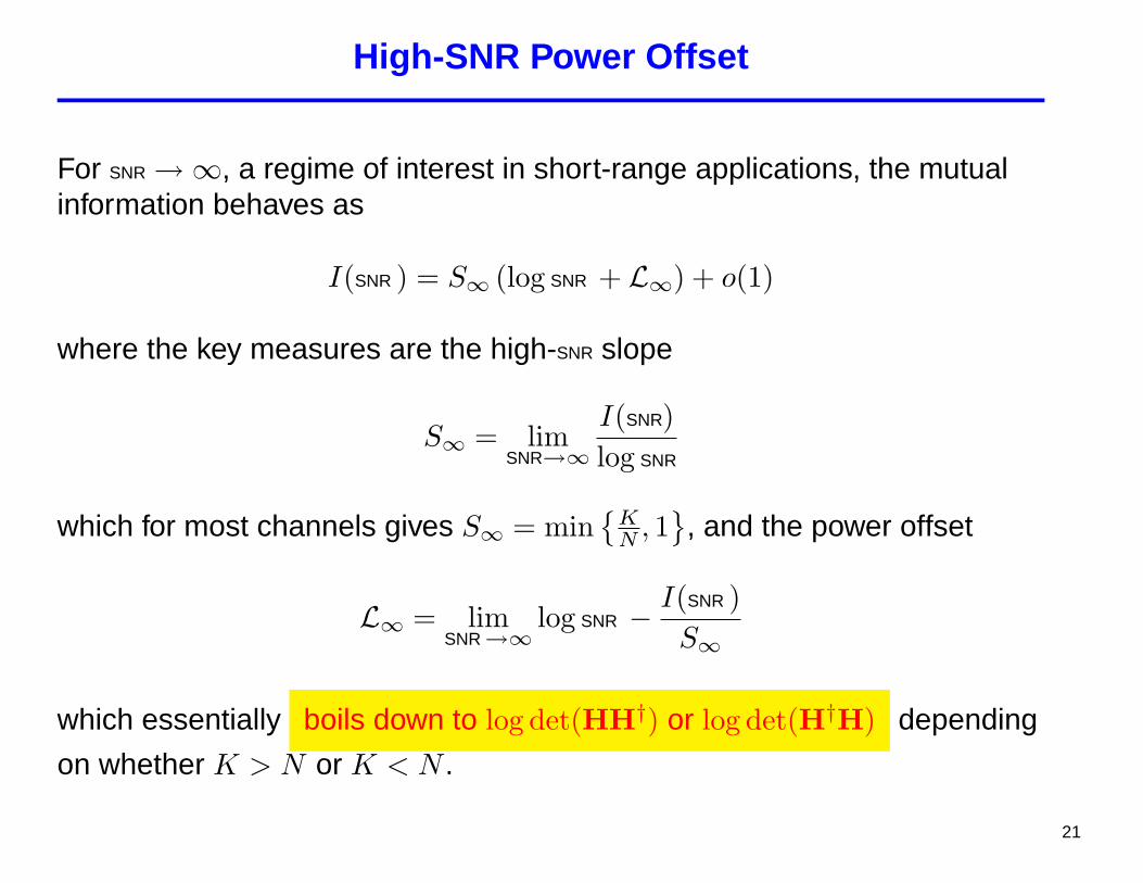
High-SNR Power Offset
For SNR →∞, a regime of interest in short-range applications, the mutualinformation behaves as
I(SNR ) = S∞ (log SNR + L∞) + o(1)
where the key measures are the high-SNR slope
S∞ = limSNR→∞
I(SNR)log SNR
which for most channels gives S∞ = min{
KN , 1
}, and the power offset
L∞ = limSNR→∞
log SNR − I(SNR )S∞
which essentially boils down to log det(HH†) or log det(H†H) depending
on whether K > N or K < N .
21
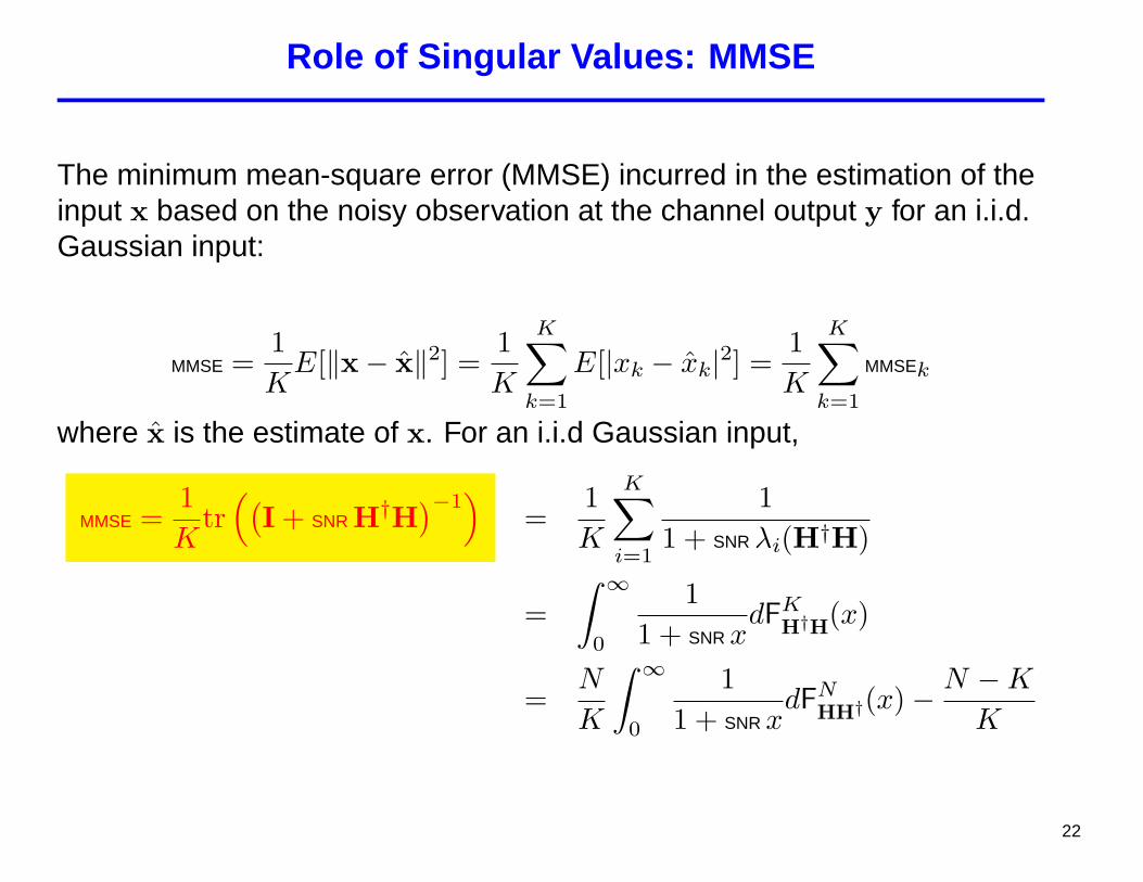
Role of Singular Values: MMSE
The minimum mean-square error (MMSE) incurred in the estimation of theinput x based on the noisy observation at the channel output y for an i.i.d.Gaussian input:
MMSE =1K
E[‖x− x‖2] =1K
K∑k=1
E[|xk − xk|2] =1K
K∑k=1
MMSEk
where x is the estimate of x. For an i.i.d Gaussian input,
MMSE =1K
tr((
I + SNR H†H)−1)
=1K
K∑i=1
11 + SNR λi(H†H)
=∫ ∞
0
11 + SNR x
dFKH†H(x)
=N
K
∫ ∞
0
11 + SNR x
dFNHH†(x)− N −K
K
22

In the Beginning ...
23

The Birth of (Nonasymptotic) Random Matrix Theory:(Wishart, 1928)
J. Wishart, “The generalized product moment distribution in samples froma normal multivariate population,” Biometrika, vol. 20 A, pp. 32–52, 1928.
Probability density function of the Wishart matrix:
HH† = h1h†1 + . . . + hnh†n
where hi are iid zero-mean Gaussian vectors.
24

Wishart Matrices
Definition 1. The m × m random matrix A = HH† is a (central)real/complex Wishart matrix with n degrees of freedom and covariancematrix Σ, (A ∼ Wm(n,Σ)), if the columns of the m × n matrix H are zero-mean independent real/complex Gaussian vectors with covariance matrixΣ.1
The p.d.f. of a complex Wishart matrix A ∼ Wm(n,Σ) for n ≥ m is
fA(B) =π−m(m−1)/2
detΣn∏m
i=1(n− i)!exp
[−tr
{Σ−1B
}]detBn−m. (1)
1If the entries of H have nonzero mean, HH† is a non-central Wishart matrix.
25

Singular Values 2: Fisher-Hsu-Girshick-Roy
The joint p.d.f. of the ordered strictly positive eigenvalues of the Wishartmatrix HH†:
• R. A. Fisher, “The sampling distribution of some statistics obtained fromnon-linear equations,” The Annals of Eugenics, vol. 9, pp. 238–249, 1939.
• M. A. Girshick, “On the sampling theory of roots of determinantalequations,” The Annals of Math. Statistics, vol. 10, pp. 203–204, 1939.
• P. L. Hsu, “On the distribution of roots of certain determinantal equations,”The Annals of Eugenics, vol. 9, pp. 250–258, 1939.
• S. N. Roy, “p-statistics or some generalizations in the analysis of varianceappropriate to multivariate problems,” Sankhya, vol. 4, pp. 381–396,1939.
26
Singular Values 2: Fisher-Hsu-Girshick-Roy
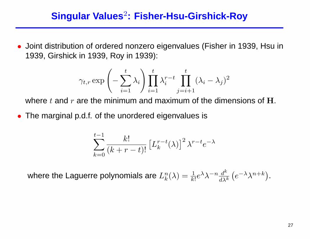
• Joint distribution of ordered nonzero eigenvalues (Fisher in 1939, Hsu in1939, Girshick in 1939, Roy in 1939):
γt,r exp
(−
t∑i=1
λi
)t∏
i=1
λr−ti
t∏j=i+1
(λi − λj)2
where t and r are the minimum and maximum of the dimensions of H.
• The marginal p.d.f. of the unordered eigenvalues is
t−1∑k=0
k!(k + r − t)!
[Lr−t
k (λ)]2
λr−te−λ
where the Laguerre polynomials are Lnk(λ) = 1
k!eλλ−n dk
dλk
(e−λλn+k
).
27

Singular Values 2: Fisher-Hsu-Girshick-Roy
0
1
2
3
4
5
0
1
2
3
4
50
0.01
0.02
0.03
0.04
0.05
0.06
0.07
0.08
Figure 1: Joint p.d.f. of the unordered positive eigenvalues of the Wishartmatrix HH† with n = 3 and m = 2.
28

Wishart Matrices: Eigenvectors
Theorem 1. The matrix of eigenvectors of Wishart matrices is uniformlydistributed on the manifold of unitary matrices ( Haar measure)
29
Unitarily invariant RMs
• Definition: An N × N self-adjoint random matrix A is called unitarilyinvariant if the p.d.f. of A is equal to that of VAV† for any unitary matrixV.
• Property: If A is unitarily invariant, it admits the following eigenvaluedecomposition:
A = UΛU†.
with U and Λ independent.
• Example
> A Wishart matrix is unitarily invariant.
> A = 12(H + H†) with H a N × N Gaussian matrix with i.i.d entries, is
unitarily invariant.
> A = UBU with U Haar matrix and B independent on U, is unitarilyinvariant.
30
Bi-Unitarily invariant RMs
• Definition: An N ×N random matrix A is called bi-unitarily invariant if itsp.d.f. equals that of UAV† for any unitary matrices U and V.
• Property: If A is a bi-unitarily invariant RM, it has a polar decompositionA = UH with
> U N ×N Haar RM.> H N ×N unitarily invariant positive-definite RM.> U and H independent.
Example:
> A complex Gaussian randon matrix with i.i.d. entries is bi-unitarilyinvariant.
> An N × K matrix Q uniformly distributed over the Stiefel manifold ofcomplex N ×K matrices such that QQ† = I.
31

The Birth of Asymptotic Random Matrix Theory
E. Wigner, “Characteristic vectors of bordered matrices with infinitedimensions,” The Annals of Mathematics, vol. 62, pp. 546–564, 1955.
W =1√N
0 +1 +1 −1 −1 +1
+1 0 −1 −1 +1 +1+1 −1 0 +1 +1 −1−1 −1 +1 0 +1 +1−1 +1 +1 +1 0 −1+1 +1 −1 +1 −1 0
As the matrix dimension N →∞, the histogram of the eigenvaluesconverges to the semicircle law:
f(x) =12π
√4− x2, − 2 < x < 2
Motivation: bypass the Schrodinger equation and explain the statistics ofexperimentally measured atomic energy levels in terms of the limitingspectrum of those random matrices.
32

Wigner Matrices: The Semicircle Law
E. Wigner, “On the distribution of roots of certain symmetric matrices,” TheAnnals of Mathematics, vol. 67, pp. 325–327, 1958.
If the upper-triangular entries are independent zero-mean randomvariables with variance 1
N (standard Wigner matrix) such that, for someconstant κ, and sufficiently large N
max1≤i≤j≤N
E[|Wi,j|4
]≤ κ
N2(2)
Then, the empirical distribution of W converges almost surely to thesemicircle law
33

The Semicircle Law
−2.5 −2 −1.5 −1 −0.5 0 0.5 1 1.5 2 2.50
0.05
0.1
0.15
0.2
0.25
0.3
The semicircle law density function compared with the histogram of the average of 100empirical density functions for a Wigner matrix of size N = 10.
34

Square matrix of iid coefficients
Girko (1984), full-circle law for the unsymmetrized matrix
H =1√N
+1 +1 +1 −1 −1 +1−1 −1 −1 −1 +1 +1+1 −1 −1 +1 +1 −1+1 −1 −1 −1 +1 +1−1 −1 +1 −1 −1 −1−1 −1 +1 +1 +1 +1
As N →∞, the eigenvalues of H are uniformly distributed on the unit disk.
−1.5 −1 −0.5 0 0.5 1 1.5−1.5
−1
−0.5
0
0.5
1
1.5
The full-circle law and the eigenvalues of a realization of a 500× 500 matrix
35
Full Circle Law
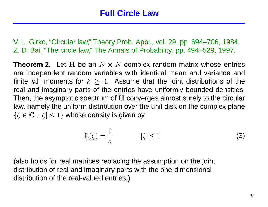
V. L. Girko, “Circular law,” Theory Prob. Appl., vol. 29, pp. 694–706, 1984.Z. D. Bai, “The circle law,” The Annals of Probability, pp. 494–529, 1997.
Theorem 2. Let H be an N × N complex random matrix whose entriesare independent random variables with identical mean and variance andfinite kth moments for k ≥ 4. Assume that the joint distributions of thereal and imaginary parts of the entries have uniformly bounded densities.Then, the asymptotic spectrum of H converges almost surely to the circularlaw, namely the uniform distribution over the unit disk on the complex plane{ζ ∈ C : |ζ| ≤ 1} whose density is given by
fc(ζ) =1π
|ζ| ≤ 1 (3)
(also holds for real matrices replacing the assumption on the jointdistribution of real and imaginary parts with the one-dimensionaldistribution of the real-valued entries.)
36

Elliptic Law (Sommers-Crisanti-Sompolinsky-Stein, 1988)
H. J. Sommers, A. Crisanti, H. Sompolinsky, and Y. Stein, Spectrum oflarge random asymmetric matrices, Physical Review Letters, vol. 60,pp. 1895- 1899, 1988.
If the off-diagonal entries are Gaussian and pairwise correlated withcorrelation coefficient ρ, the eigenvalues are asymptotically uniformlydistributed on an ellipse in the complex plane whose axes coincide with thereal and imaginary axes and have radii 1 + ρ and 1− ρ.
37

What About the Singular Values?
38

Asymptotic Distribution of Singular Values:Quarter circle law
Consider an N ×N matrix H whose entries are independent zero-meancomplex (or real) random variables with variance 1
N , the asymptoticdistribution of the singular values converges to
q(x) =1π
√4− x2, 0 ≤ x ≤ 2 (4)
39
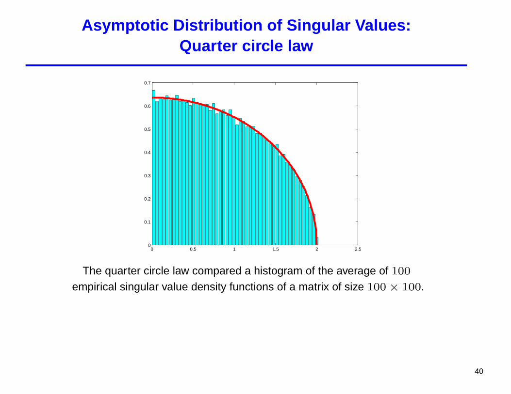
Asymptotic Distribution of Singular Values:Quarter circle law
0 0.5 1 1.5 2 2.50
0.1
0.2
0.3
0.4
0.5
0.6
0.7
The quarter circle law compared a histogram of the average of 100empirical singular value density functions of a matrix of size 100× 100.
40
Minimum Singular Value of Gaussian Matrix
• A. Edelman, Eigenvalues and condition number of random matrices. PhDthesis, Dept. Mathematics, MIT, Cambridge, MA, 1989.
• J. Shen, “On the singular values of Gaussian random matrices,” LinearAlgebra and its Applications, vol. 326, no. 1-3, pp. 1–14, 2001.
Theorem 3. The minimum singular value of an N × N standard complexGaussian matrix H satisfies
limN→∞
P [Nσmin ≥ x] = e−x−x2/2. (5)
41

Marcenko-Pastur Law
• V. A. Marcenko and L. A. Pastur, “Distributions of eigenvalues for somesets of random matrices,” Math USSR-Sbornik, vol. 1, pp. 457–483,1967.
U. Grenander and J. W. Silverstein, “Spectral analysis of networks withrandom topologies,” SIAM J. of Applied Mathematics, vol. 32, pp. 449–519, 1977.
K. W. Wachter, “The strong limits of random matrix spectra for samplematrices of independent elements,” The Annals of Probability, vol. 6,no. 1, pp. 1–18, 1978.
J. W. Silverstein and Z. D. Bai, “On the empirical distribution ofeigenvalues of a class of large dimensional random matrices,” J. ofMultivariate Analysis, vol. 54, pp. 175–192, 1995.
Y. L. Cun, I. Kanter, and S. A. Solla, “Eigenvalues of covariance matrices:Application to neural-network learning,” Physical Review Letters, vol. 66,pp. 2396–2399, 1991.
42

Rediscovering/Strenghtening the Mar cenko-Pastur Law
• V. A. Marcenko and L. A. Pastur, “Distributions of eigenvalues for somesets of random matrices,” Math USSR-Sbornik, vol. 1, pp. 457–483,1967.
• U. Grenander and J. W. Silverstein, “Spectral analysis of networks withrandom topologies,” SIAM J. of Applied Mathematics, vol. 32, pp. 449–519, 1977.
• K. W. Wachter, “The strong limits of random matrix spectra for samplematrices of independent elements,” The Annals of Probability, vol. 6,no. 1, pp. 1–18, 1978.
• J. W. Silverstein and Z. D. Bai, “On the empirical distribution ofeigenvalues of a class of large dimensional random matrices,” J. ofMultivariate Analysis, vol. 54, pp. 175–192, 1995.
• Y. L. Cun, I. Kanter, and S. A. Solla, “Eigenvalues of covariance matrices:Application to neural-network learning,” Physical Review Letters, vol. 66,pp. 2396–2399, 1991.
43

Marcenko-Pastur Law
V. A. Marcenko and L. A. Pastur, “Distributions of eigenvalues for somesets of random matrices,” Math USSR-Sbornik, vol. 1, pp. 457–483, 1967.
If N ×K-matrix H has zero-mean i.i.d. entries with variance 1N , the
asymptotic ESD of HH† found in (Marcenko-Pastur, 1967) is
fβ(x) = [1− β]+ δ(x) +
√[x− a]+[b− x]+
2πx
where[z]+ = max{0, z},
and
a =(1−
√β)2
b =(1 +
√β)2
.
K
N→ β
44
Marcenko-Pastur Law
V. A. Marcenko and L. A. Pastur, “Distributions of eigenvalues for somesets of random matrices,” Math USSR-Sbornik, vol. 1, pp. 457–483, 1967.
If N ×K-matrix H has zero-mean i.i.d. entries with variance 1N , the
asymptotic ESD of HH† found in (Marcenko-Pastur, 1967) is
fβ(x) = [1− β]+ δ(x) +
√[x− a]+[b− x]+
2πx
(Bai 1999) The results also holds if only a unit second-moment condition isplaced on the entries of H and
1K
∑E[|Hi,j|2 1 {|Hi,j| ≥ δ}
]→ 0
for any δ > 0 (Lindeberg-type condition on the whole matrix).
45

Nonzero-Mean Matrices
Lemma: (Yin 1986, Bai 1999): For any N ×K matrices A and B,
supx≥0
|FNAA†(x)− FN
BB†(x)| ≤ rank(A−B)N
.
Lemma: (Yin 1986, Bai 1999): For any N ×N Hermitian matrices A and B,
supx≥0
|FNA (x)− FN
B (x)| ≤ rank(A−B)N
.
Using these Lemmas, all results illustrated so far can be extended tomatrices whose mean has rank r where r > 1 but such that
limN→∞
r
N= 0.
46
Generalizations needed!
• Correlated EntriesH =
√ΦRS
√ΦT
S: N × K matrix whose entries are independent complex randomvariables (arbitrarily distributed)
ΦR: N × N either deterministic or random matrix (whose asymptoticspectrum of converges a. s. to a compactly supported measure).
ΦT: K × K either deterministic or random matrix matrix whoseasymptotic spectrum converges a. s. to a compactly supportedmeasure.
• Non-identically Distributed Entries
H be an N × K complex random matrix with independent entries(arbitrarily distributed) with identical means.
Var[Hi,j] =Gi,j
Nwith Gi,j uniformly bounded.
Special case : Doubly Regular Channels
47

Transforms
1. Stieltjes transform
2. η transform
3. Shannon transform
4. R-transform
5. S-transform
48
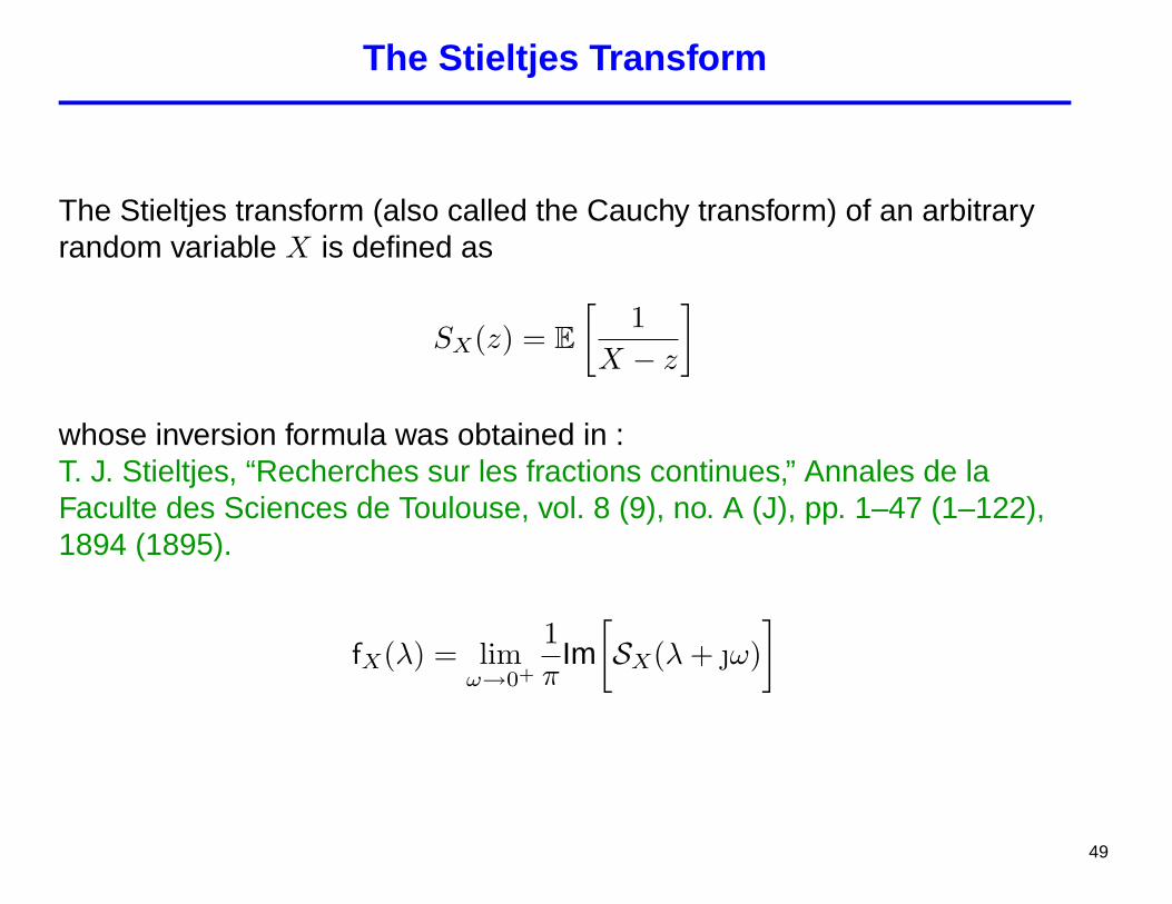
The Stieltjes Transform
The Stieltjes transform (also called the Cauchy transform) of an arbitraryrandom variable X is defined as
SX(z) = E[
1X − z
]whose inversion formula was obtained in :T. J. Stieltjes, “Recherches sur les fractions continues,” Annales de laFaculte des Sciences de Toulouse, vol. 8 (9), no. A (J), pp. 1–47 (1–122),1894 (1895).
fX(λ) = limω→0+
1π
Im[SX(λ + ω)
]
49

The η-Transform [Tulino-Verdu 2004]
The η-transform of a nonnegative random variable X is given by
ηX(γ) = E[
11 + γX
]where γ is a nonnegative real number, and thus, 0 < ηX(γ) ≤ 1.
Note:
ηX(γ) =∞∑
k=0
(−γ)kE[Xk],
50
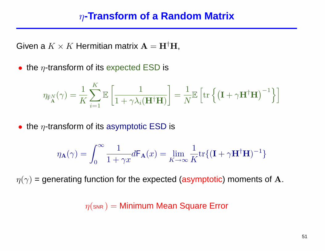
η-Transform of a Random Matrix
Given a K ×K Hermitian matrix A = H†H,
• the η-transform of its expected ESD is
ηFNA(γ) =
1K
K∑i=1
E[
11 + γλi(H†H)
]=
1N
E[tr{(
I + γH†H)−1}]
• the η-transform of its asymptotic ESD is
ηA(γ) =∫ ∞
0
11 + γx
dFA(x) = limK→∞
1K
tr{(I + γH†H)−1}
η(γ) = generating function for the expected (asymptotic) moments of A.
η(SNR ) = Minimum Mean Square Error
51

The Shannon Transform [Tulino-Verdu 2004]
The Shannon transform of a nonnegative random variable X is defined as
VX(γ) = E[log(1 + γX)]
where γ > 0.
• The Shannon transform gives the capacity of various noisy coherentcommunication channels.
52

Shannon Transform of a Random Matrix
Given a N ×N Hermitian matrix A = HH†,
• the Shannon transform of its expected ESD is
VFNA(γ) =
1N
E [log det (I + γA)]
• the Shannon transform of its asymptotic ESD is
VA(γ) = limN→∞
1N
log det (I + γA)
I(SNR ,HH†) = V(SNR )
53

Stieltjes, Shannon and η
γ
log e
d
dγVX(γ) = 1− 1
γSX
(−1
γ
)= 1− ηX(γ)
m
SNRd
dSNRI(SNR ) =
K
N(1− MMSE)
54

Stieltjes, Shannon and η
γ
log e
d
dγVX(γ) = 1− 1
γSX
(−1
γ
)= 1− ηX(γ)
m
SNRd
dSNRI(SNR ) =
K
N(1− MMSE)
55
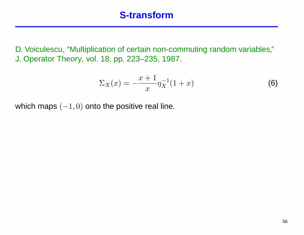
S-transform
D. Voiculescu, “Multiplication of certain non-commuting random variables,”J. Operator Theory, vol. 18, pp. 223–235, 1987.
ΣX(x) = −x + 1x
η−1X (1 + x) (6)
which maps (−1, 0) onto the positive real line.
56

S-transform: Key Theorem
♣O. Ryan, On the limit distributions of random matrices with independent or free entries,Com. in Mathematical Physics, vol. 193, pp. 595-626, 1998.
♠F. Hiai and D. Petz, Asymptotic freeness almost everywhere for random matrices, ActaSci. Math. Szeged, vol. 66, pp. 801-826, 2000.
Let A and B be independent random matrices, if either:
♠ B is unitarily or bi-unitarily invariant,
♣ or both A and B have i.i.d entries
then S-transform of the spectrum of AB is :
ΣAB(x) = ΣA(x)ΣB(x)
and
ηAB(γ) = ηA
(γ
ΣB(ηAB(γ)− 1)
)57

S-transform: Example
LetH = CQ
where:> K ≤ N
> Q is an N × K matrix independent of C and uniformly distributed overthe Stiefel manifold of complex N ×K matrices such that QQ† = I.
Since Q is bi-unitarily invariant then
ηCQQ†C†(SNR ) = ηCC†
(SNR
β − 1 + ηCQQ†C†
ηCQQ†C†(SNR )
)and
VCQQ†C†(γ) =∫ SNR
0
1x(1− ηCQQ†C†(x)) dx
58

Downlink MC-CDMA with Orthogonal Sequences and equal-power
y = CQAx + n,
where:> Q = the orthogonal spreading sequences
> A = the K ×K diagonal matrix of transmitted amplitudes with A = I> C = the N ×N matrix of fading coefficients.
1K
K∑k=1
MMSEka.s.→ ηQ†C†CQ(SNR ) = 1− 1
β(1− ηCQQ†C†(SNR ))
An alternative characterization of the Shannon-transform (inspired by the optimality bysuccessive cancellation with MMSE ) is
VCQQ†C†(γ) = β E [log (1 + ,Y)ג γ))]
with,y)ג γ)
1 + ,y)ג γ)= E
"γ|C|2
β y γ|C|2 + 1 + (1− β y)ג(y, γ)
#
where Y is a random variable uniform on [0, 1].
59

R-transform
D. Voiculescu, “Addition of certain non-commuting random variables,” J.Funct. Analysis, vol. 66, pp. 323–346, 1986.
RX(z) = S−1X (−z)− 1
z. (7)
R-transform and η-transform
The R-transform (restricted to the negative real axis) of a non-negativerandom variable X is given by
RX(ϕ) =ηX(γ)− 1
ϕ
with γ and ϕ satisfying ϕ = −γ ηX(γ)
60
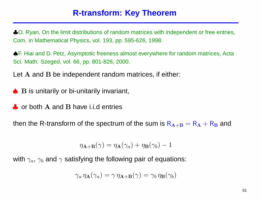
R-transform: Key Theorem
♣O. Ryan, On the limit distributions of random matrices with independent or free entries,Com. in Mathematical Physics, vol. 193, pp. 595-626, 1998.
♠F. Hiai and D. Petz, Asymptotic freeness almost everywhere for random matrices, ActaSci. Math. Szeged, vol. 66, pp. 801-826, 2000.
Let A and B be independent random matrices, if either:
♠ B is unitarily or bi-unitarily invariant,
♣ or both A and B have i.i.d entries
then the R-transform of the spectrum of the sum is RA+B = RA + RB and
ηA+B(γ) = ηA(γa) + ηB(γb)− 1
with γa, γb and γ satisfying the following pair of equations:
γa ηA(γa) = γ ηA+B(γ) = γb ηB(γb)
61

Random Quadratic Forms
Z. D. Bai and J. W. Silverstein, “No eigenvalues outside the support of thelimiting spectral distribution of large dimensional sample covariancematrices,” The Annals of Probability, vol. 26, pp. 316–345, 1998.
Theorem 4. Let the components of the N -dimensional vector x be zero-mean and independent with variance 1
N . For any N × N nonnegativedefinite random matrix B independent of x whose spectrum convergesalmost surely,
limN→∞
x† (I + γB)−1 x = ηB(γ) a.s. (8)
limN→∞
x† (B− zI)−1 x = SB(z) a.s. (9)
62
Rationale
Stieltjes: Description of asymptotic distribution of singular values +tool for proving results (Marcenko-Pastur (1967))
η: Description of asymptotic distribution of singular values +signal processing insight
Shannon: Description of asymptotic distribution of singular values +information theory insight
63
Non-asymptotic Shannon Transform
Example: For N ×K-matrix H having zero-mean i.i.d. Gaussian entries:
V(SNR ) =t−1∑k=0
k∑`1=0
k∑`2=0
(k
`1
)(k + r − t)!(−1)`1+`2I`1+`2+r−t(SNR )(k − `2)!(r − t + `1)!(r − t + `2)!`2!
I0(SNR ) = −e1
SNR Ei(− 1SNR
)
In(SNR ) = nIn−1(SNR ) + (−SNR )−n
(I0(SNR ) +
n∑k=1
(k − 1)! (−SNR )k
)
For the η-Transform
η(SNR ) = 1− SNR
β
d
dSNRV(SNR )
64
Asymptotics
• K →∞
• N →∞
• KN → β
65
Shannon and η-Transform of Mar cenko-Pastur Law
Example: The Shannon transform of the Marcenko-Pastur law is
V(SNR ) = log(
1 + SNR − 14F (SNR , β)
)+
1β
log(
1 + SNR β − 14F (SNR , β)
)− log e
4 β SNRF (SNR , β)
where
F(x, z) =(√
x(1 +√
z)2 + 1−√
x(1−√
z)2 + 1)2
while its η-transform is
ηHH†(SNR ) =(
1− F(SNR , β)4 SNR
)
66

Asymptotics
Shannon Capacity = VFNHH†
(SNR ) =1N
N∑i=1
log(1 + SNR λi(HH†)
)
N = 50
SNR SNR
SNRSNR
N = 3 N = 5
N = 15
0 2 4 6 8 100
1
2
3
4
0 2 4 6 8 100
1
2
3
4
0 2 4 6 8 100
1
2
3
4
0 2 4 6 8 100
1
2
3
4
β = 1 for sizes: N = 3, 5, 15, 50
67
Asymptotics
Distribution Insensitivity: The asymptotic eigenvalue distribution doesnot depend on the distribution with which the independent matrixcoefficients are generated.
“Ergodicity”: The eigenvalue histogram of one matrix realizationconverges almost surely to the asymptotic eigenvalue distribution.
Speed of Convergence: 8 = ∞.
68
Marcenko-Pastur Law: Applications
• Unfaded Equal-Power DS-CDMA
• Canonical model (i.i.d. Rayleigh fading MIMO channels)
• Multi-Carrier CDMA channels whose sequences have i.i.d. entries
69

More General Models
• Correlated EntriesH =
√ΦRS
√ΦT
S: N × K matrix whose entries are independent complex randomvariables (arbitrarily distributed) with identical means and variance 1
N .ΦR: N × N random matrix whose asymptotic spectrum of converges a.
s. to a compactly supported measure.ΦT: K ×K random matrix whose asymptotic spectrum converges a. s.
to a compactly supported measure.
• Non-identically Distributed Entries
H be an N × K complex random matrix with independent entries(arbitrarily distributed) with identical means.
Var[Hi,j] =Gi,j
Nwith Gi,j uniformly bounded.
Special case : Doubly Regular Channels
70

Doubly Regular Matrices [Tulino-Lozano-Verdu,2005]
Definition: An N ×K matrix P is asymptotically mean row-regular if
limK→∞
1K
K∑j=1
Pi,j
is independent of i as KN → β.
Definition: P is asymptotically mean column-regular if its transpose isasymptotically mean row-regular.
Definition: P is asymptotically mean doubly-regular if it is bothasymptotically mean row-regular and asymptotically mean column-regular.
• If the limits limN→∞
1N
N∑i=1
Pi,j = limK→∞
1K
K∑j=1
Pi,j = 1 then P is standard
asymptotically mean doubly-regular.
71

Regular Matrices: Example
• An N ×K rectangular Toeplitz matrix
Pi,j = ϕ(i− j)
with K ≥ N is an asymptotically mean row-regular matrix.
• If either the function ϕ is periodic or N = K, then the Toeplitz matrix isasymptotically mean doubly-regular.
72
Double Regularity: Engineering Insight
text
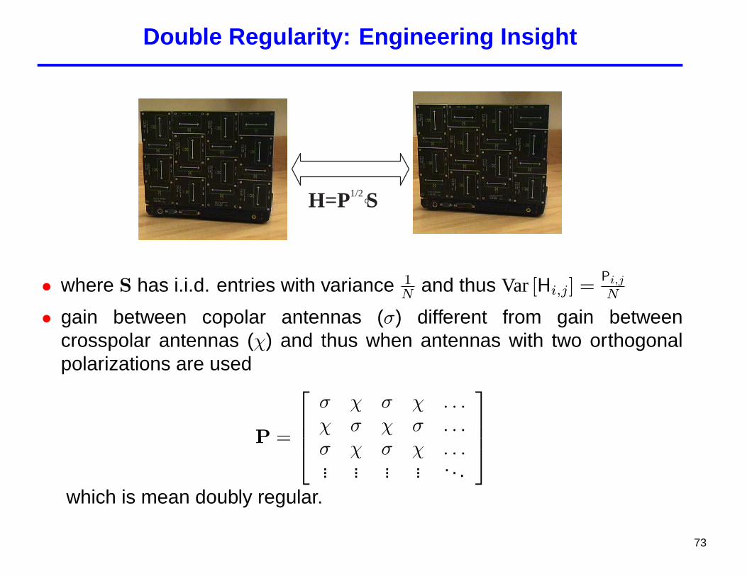
H=P S 1/2 o
• where S has i.i.d. entries with variance 1N and thus Var [Hi,j] = Pi,j
N
• gain between copolar antennas (σ) different from gain betweencrosspolar antennas (χ) and thus when antennas with two orthogonalpolarizations are used
P =
σ χ σ χ . . .χ σ χ σ . . .σ χ σ χ . . .... ... ... ... . . .
which is mean doubly regular.
73
Asymptotic ESD of a Doubly-Regular Matrix[Tulino-Lozano-Verdu, 2005]
Theorem: Define an N ×K complex random matrix H whose entries
• are independent (arbitrarily distributed) satisfying the Lindeberg conditionand with identical means.
• have variancesVar [Hi,j] =
Pi,j
Nwith P an N × K deterministic standard asymptotically doubly-regularmatrix whose entries are uniformly bounded for any N .
The ESD of H†H converges a.s. to the Marcenko-Pastur law.
This result extends to matrices H = H0 + H whose mean has rank r > 1such that
limN→∞
r
N= 0.
74
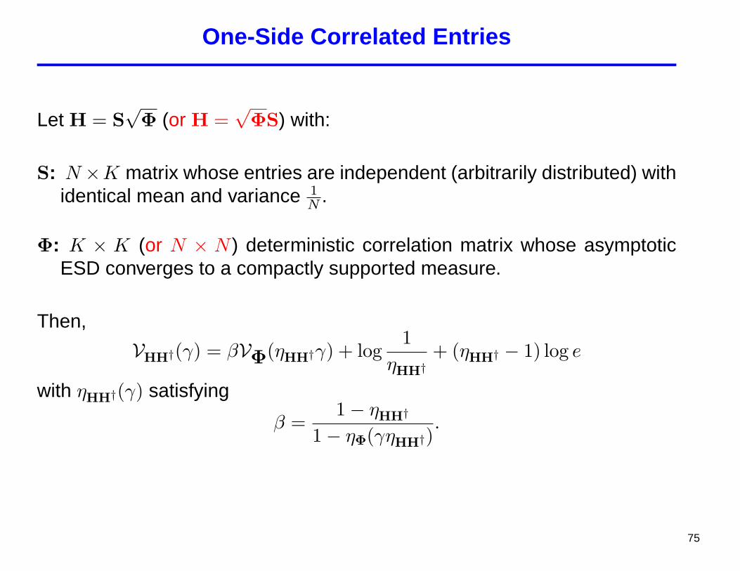
One-Side Correlated Entries
Let H = S√
Φ (or H =√
ΦS) with:
S: N ×K matrix whose entries are independent (arbitrarily distributed) withidentical mean and variance 1
N .
Φ: K × K (or N × N ) deterministic correlation matrix whose asymptoticESD converges to a compactly supported measure.
Then,
VHH†(γ) = βVΦ(ηHH†γ) + log1
ηHH†+ (ηHH† − 1) log e
with ηHH†(γ) satisfying
β =1− ηHH†
1− ηΦ(γηHH†).
75
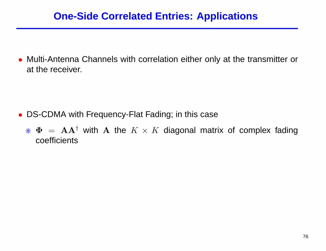
One-Side Correlated Entries: Applications
• Multi-Antenna Channels with correlation either only at the transmitter orat the receiver.
• DS-CDMA with Frequency-Flat Fading; in this case
> Φ = AA† with A the K × K diagonal matrix of complex fadingcoefficients
76
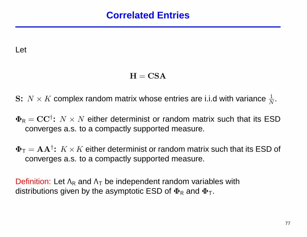
Correlated Entries
Let
H = CSA
S: N ×K complex random matrix whose entries are i.i.d with variance 1N .
ΦR = CC†: N × N either determinist or random matrix such that its ESDconverges a.s. to a compactly supported measure.
ΦT = AA†: K×K either determinist or random matrix such that its ESD ofconverges a.s. to a compactly supported measure.
Definition: Let ΛR and ΛT be independent random variables withdistributions given by the asymptotic ESD of ΦR and ΦT.
77

Correlated Entries: Applications
• Multi-Antenna Channels with correlation at the transmitter and receiver(Separable correlation model); in this case:
> ΦR = the receive correlation matrix respectively,
> ΦT = the transmit correlation matrix.
• Downlink MC-CDMA with frequency-selective fading and i.i.d sequences;in this case:
> C = the N × N diagonal matrix containing fading coefficient for eachsubcarrier,
> A = the K×K deterministic diagonal matrix containing the amplitudesof the users.
78
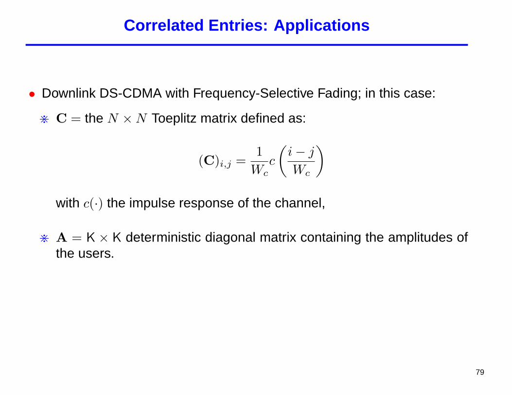
Correlated Entries: Applications
• Downlink DS-CDMA with Frequency-Selective Fading; in this case:
> C = the N ×N Toeplitz matrix defined as:
(C)i,j =1
Wcc
(i− j
Wc
)with c(·) the impulse response of the channel,
> A = K × K deterministic diagonal matrix containing the amplitudes ofthe users.
79
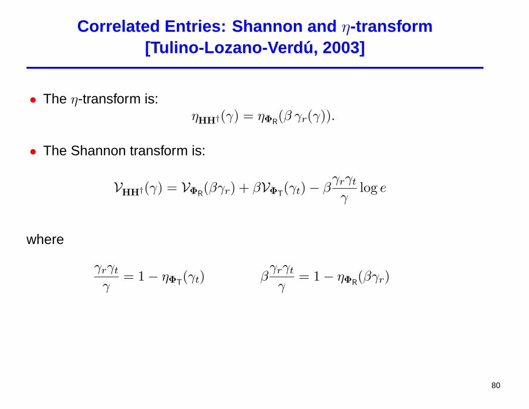
Correlated Entries: Shannon and η-transform[Tulino-Lozano-Verdu, 2003]
• The η-transform is:ηHH†(γ) = ηΦR
(β γr(γ)).
• The Shannon transform is:
VHH†(γ) = VΦR(βγr) + βVΦT
(γt)− βγrγt
γlog e
where
γrγt
γ= 1− ηΦT
(γt) βγrγt
γ= 1− ηΦR
(βγr)
80
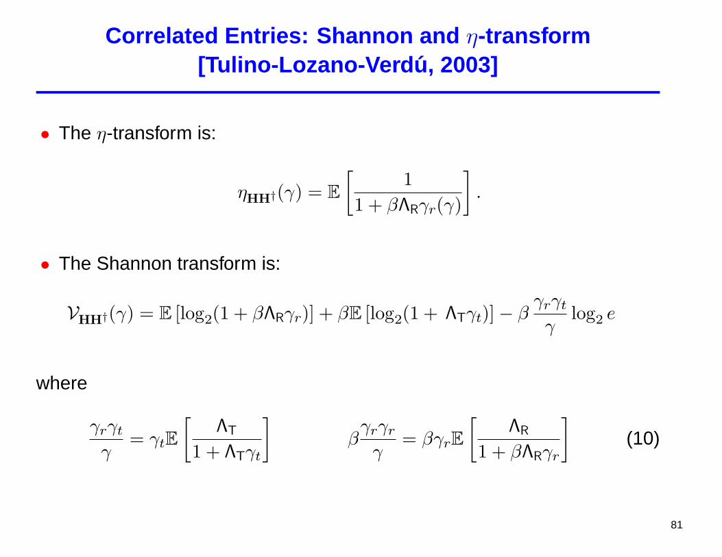
Correlated Entries: Shannon and η-transform[Tulino-Lozano-Verdu, 2003]
• The η-transform is:
ηHH†(γ) = E[
11 + βΛRγr(γ)
].
• The Shannon transform is:
VHH†(γ) = E [log2(1 + βΛRγr)] + βE [log2(1 + ΛTγt)]− βγrγt
γlog2 e
where
γrγt
γ= γtE
[ΛT
1 + ΛTγt
]β
γrγr
γ= βγrE
[ΛR
1 + βΛRγr
](10)
81
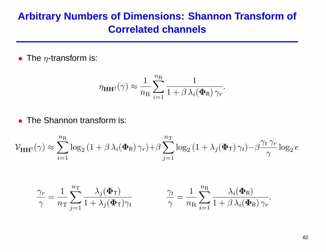
Arbitrary Numbers of Dimensions: Shannon Transform ofCorrelated channels
• The η-transform is:
ηHH†(γ) ≈ 1nR
nR∑i=1
11 + β λi(ΦR) γr
.
• The Shannon transform is:
VHH†(γ) ≈nR∑i=1
log2 (1 + β λi(ΦR) γr)+β
nT∑j=1
log2 (1 + λj(ΦT) γt)−βγt γr
γlog2 e
γr
γ=
1nT
nT∑j=1
λj(ΦT)1 + λj(ΦT)γt
γt
γ=
1nR
nR∑i=1
λi(ΦR)1 + β λi(ΦR) γr
.
82
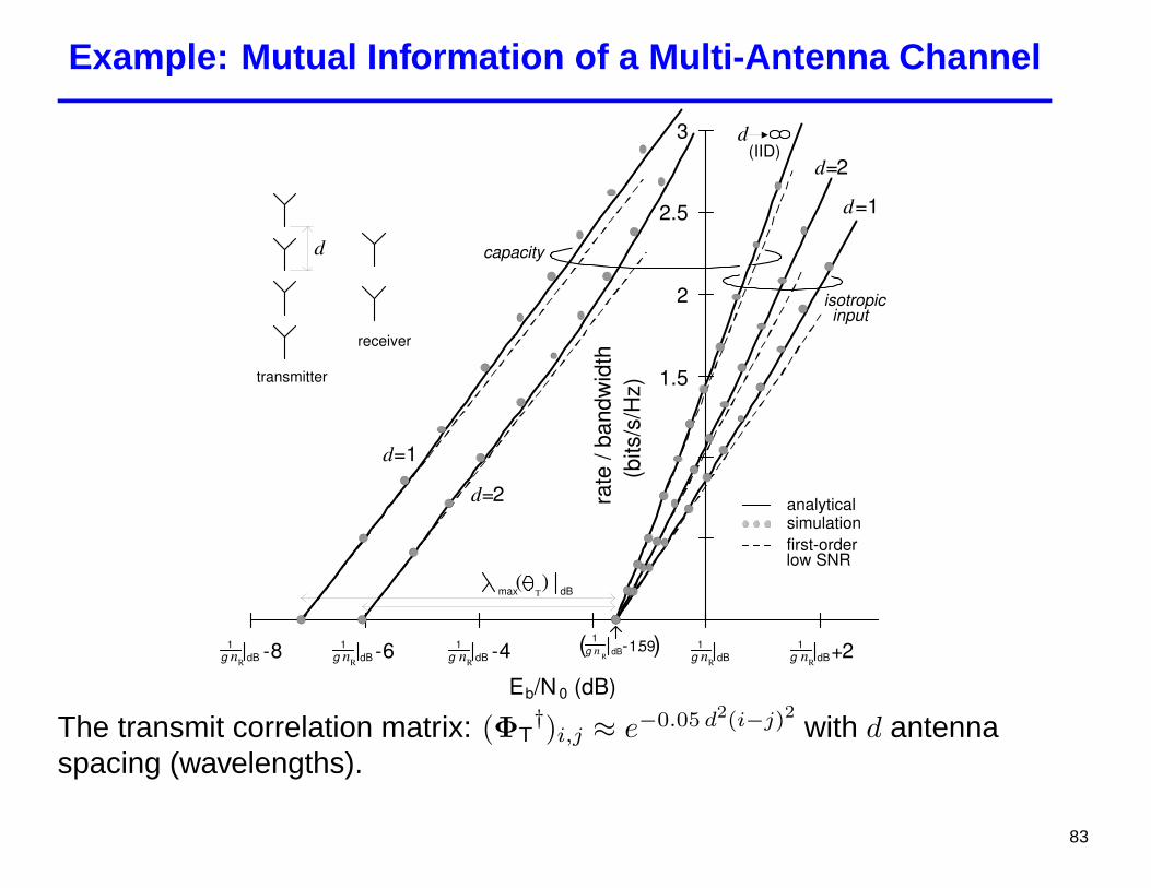
Example: Mutual Information of a Multi-Antenna Channel
.
(IID)
simulation first-order low SNR
analytical
.
d 3
1.5
2
2.5
d = 2
d =1
d =1
d = 2
capacity
isotropic input
d
transmitter
receiver
max ( )
T dB
-8 -6 -4 -2 0 2
E b /N 0 (dB)
rate
/ ba
ndw
idth
(b
its/s
/Hz)
g n R
1 dB - 6 g n R
1 dB - 4 g n R
1 dB - 8 g n R
1 dB + 2 g n R
1 dB
g n R
1 dB - 1. 59 ( )
Figure 3: C( Eb
N0) and spectral efficiency with an isotropic input, parameterized by d. Trans-
mitter is a 4-antenna ULA with antenna spacing d (wavelengths), receiver has 2 uncorre-lated antennas. Power angular spectrum at the transmitter is Gaussian (broadside) with2◦ spread. Solid lines indicate analytical solution, circles indicate simulation (Rayleighfading), dashed lines indicate low-SNR expansion.
29
The transmit correlation matrix: (ΦT†)i,j ≈ e−0.05 d2(i−j)2 with d antenna
spacing (wavelengths).
83

Correlated Entries (Hanly-Tse, 2001)
• S be a N ×K matrix with i.i.d entries
• A` = diag{A1,`, . . . ,AK,`} where {Ak,`} are i.i.d. random variables
• S be a NL×K matrix with i.i.d entries
• P a K×K diagonal matrix whose k-th diagonal entry (P)k,k =∑L
`=1 A2k,`.
The distribution of the singular values of the matrix
H =
SA1
· · ·SAL
(11)
is the same as the distribution of the singular values of the matrix
S√
P
Applications: DS-CDMA with Flat Fading and Antenna Diversity: {Ak,`} are the i.i.d.fading coefficients of the kth user at the `th antenna and S is the signature matrix.
Engineering interpretation: the effective spreading gain = the CDMA spreading gain ×the number of receive antennas
84

Non-identically Distributed Entries
Let H be an N ×K complex random matrix:
• Entries are independent (arbitrarily distributed) satisfying the Lindebergcondition and with identical means,
•Var[Hi,j] =
Pi,j
Nwhere P is an N × K deterministic matrix whose entries are uniformlybounded.
85
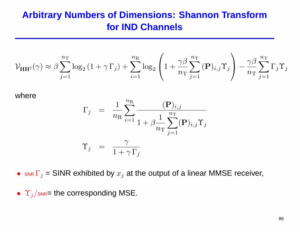
Arbitrary Numbers of Dimensions: Shannon Transformfor IND Channels
VHH†(γ) ≈ β
nT∑j=1
log2 (1 + γ Γj) +nR∑i=1
log2
1 +γβ
nT
nT∑j=1
(P)i,jΥj
− γβ
nT
nT∑j=1
ΓjΥj
where
Γj =1
nR
nR∑i=1
(P)i,j
1 + β1
nT
nT∑j=1
(P)i,jΥj
Υj =γ
1 + γ Γj
• SNR Γj = SINR exhibited by xj at the output of a linear MMSE receiver,
• Υj/SNR= the corresponding MSE.
86
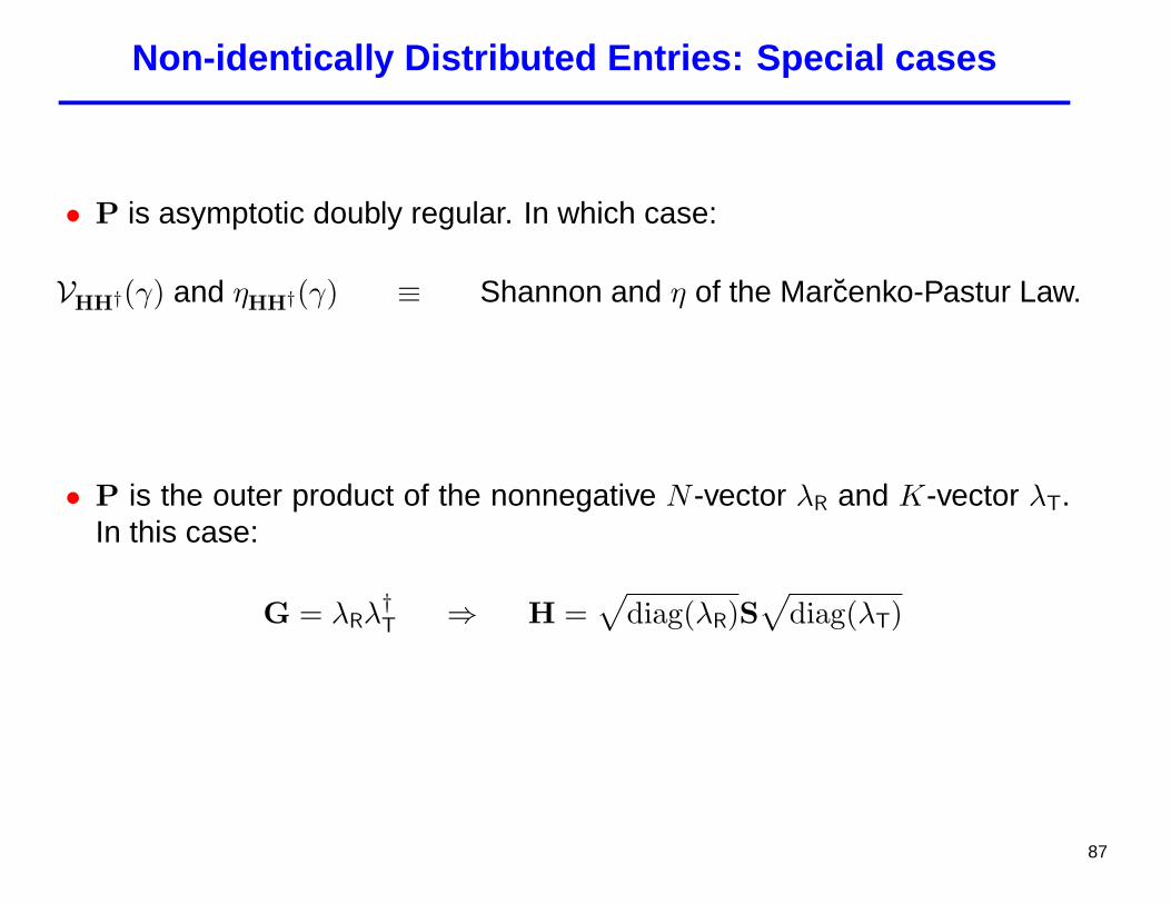
Non-identically Distributed Entries: Special cases
• P is asymptotic doubly regular. In which case:
VHH†(γ) and ηHH†(γ) ≡ Shannon and η of the Marcenko-Pastur Law.
• P is the outer product of the nonnegative N -vector λR and K-vector λT.In this case:
G = λRλ†T ⇒ H =
√diag(λR)S
√diag(λT)
87

Non-identically Distributed Entries: Applications
• MC-CDMA frequency-selective fading and i.i.d sequences (Uplink andDownlink).
• Uplink DS-CDMA with Frequency-Selective Fading:
L. Li, A. M. Tulino, and S. Verdu, Design of reduced-rank MMSE multiuser detectorsusing random matrix methods, IEEE Trans. on Information Theory, vol. 50, June 2004.
J. Evans and D. Tse, Large system performance of linear multiuser receivers inmultipath fading channels, IEEE Trans. on Information Theory, vol. 46, Sep. 2000.
J. M. Chaufray, W. Hachem, and P. Loubaton, Asymptotic analysis of optimum andsub-optimum CDMA MMSE receivers, Proc. IEEE Int. Symp. on Information Theory(ISIT02), p. 189, July 2002.
88

Non-identically Distributed Entries: Applications
• Multi-Antenna Channels with
> Polarization Diversity:
H =√
P ◦Hw
where Hw is zero-mean i.i.d. Gaussian and P is a deterministic matrixwith nonnegative entries.(P)i,j is the power gain between the jth transmit and ith receiveantennas, determined by their relative polarizations.
> Non-separable Correlations
H = UHwU†
where UR and UT are unitary while the entries of H are independentzero-mean Gaussian. A more restrictive case is when UR and UT are Fouriermatrices.This model is advocated and experimentally supported in W. Weichselberger et all,A stochastic mimo channel model with joint correlation of both link ends, IEEE Trans.on Wireless Com., vol. 5, no. 1, pp. 90–100, 2006.
89

Example: Mutual Information of a Multi-Antenna Channel
4
6
2
12
8
10
.
simulation analytical
G=0.4 3.6 0.50.3 1 0.2
-10 -5 0 5 10 15 20
SNR (dB)
Mut
ual I
nfor
mat
ion
(bits
/s/H
z)
90

Ergodic Regime
• {Hi} varies ergodically over the duration of a codeword.
• The quantity of interest is then the mutual information averaged over thefading, E
[I(SNR ,HΦH†)
], with
I(SNR ,HΦH†) =1N
log det(I + SNR HΦH†)
91

Non-ergodic Conditions
• Often, however, H is held approximately constant during the span of acodeword
• Outage capacity (cumulative distribution of mutual information),
Pout(R) = P[log det(I + SNR HH†) < R]
• The normalized mutual information converges a.s. to its expectation asK, N →∞ (hardening / self-averaging)
1N
log det(I + SNR HH†) a.s.→ VHH†(SNR ) = limN→∞
1N
E[log det(I + SNR HH†)]
However, non-normalized mutual information
I(SNR ,HH†) = log det(I + SNR HH†)
still suffers random fluctuations that, while small relative to the mean, arevital to the outage capacity.
92
CLT for Linear Spectral Statistics
Z. D. Bai and J. W. Silverstein, CLT of linear spectral statistics of largedimensional sample covariance matrices, Annals of Probability, vol. 32, no.1A, pp. 553605, 2004.
93
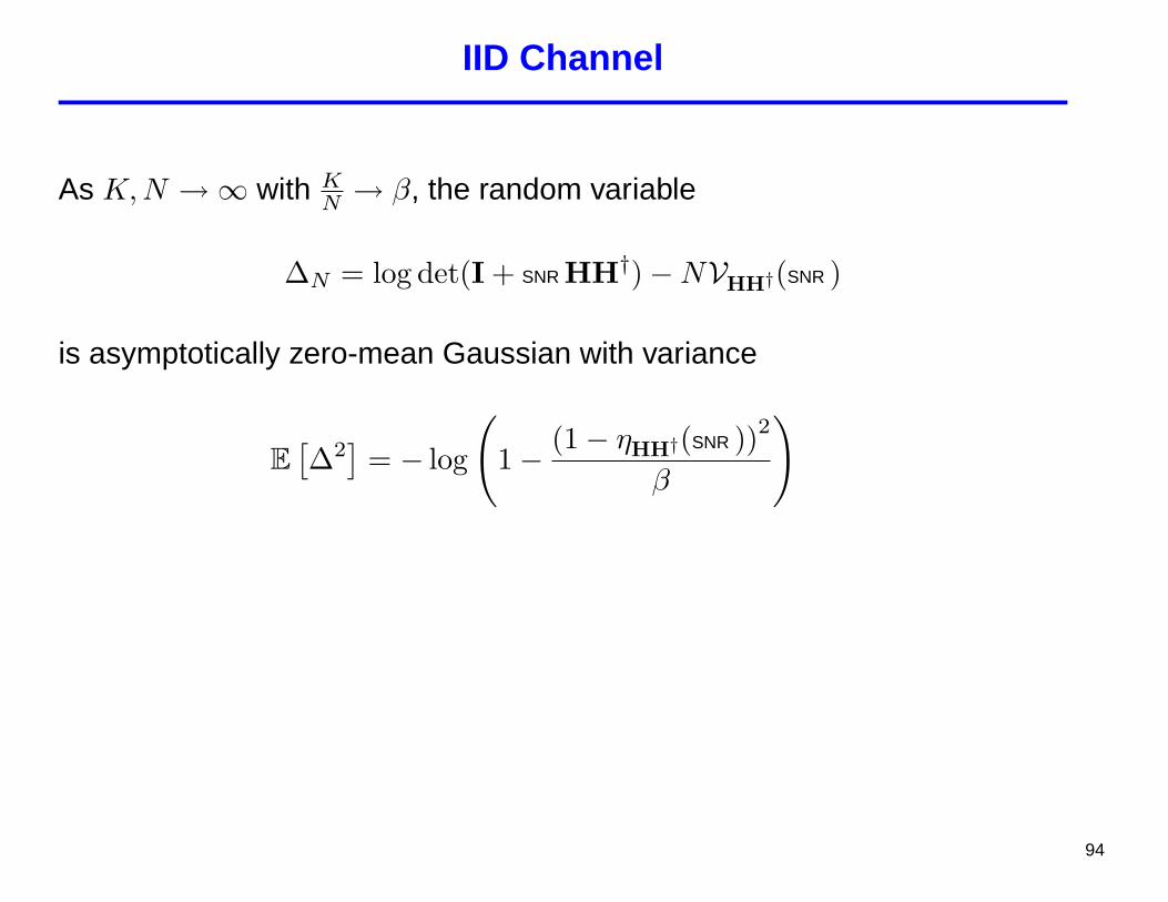
IID Channel
As K, N →∞ with KN → β, the random variable
∆N = log det(I + SNR HH†)−NVHH†(SNR )
is asymptotically zero-mean Gaussian with variance
E[∆2]
= − log
(1− (1− ηHH†(SNR ))2
β
)
94
IID Channel
• For fixed numbers of antennas, mean and variance of the mutualinformation of the IID channel given by [Smith & Shafi ’02] and [Wang& Giannakis ’04]. Approximate normality observed numerically.
• Arguments supporting the asymptotic normality of the cumulativedistribution of mutual information given:
> in [Hochwald et al. ’04], for SNR → 0 or SNR →∞.
> in [Moustakas et al. ’03] using the replica method from statisticalphysics (not yet fully rigorized).
> in [Kamath et al. ’02], asymptotic normality proved rigorously for anySNR using Bai & Silverstein’s CLT.
95
One-Side Correlated Wireless Channel ( H = S√
ΦT)[Tulino-Verdu,2004]
Theorem: As K, N →∞ with KN → β, the random variable
∆N = log det(I + SNR SΦTS†)−NVSΦTS†(SNR )
is asymptotically zero-mean Gaussian with variance
E[∆2] = − log
1− β E
( TSNR ηSΦTS†(SNR )1 + TSNR ηSΦTS†(SNR )
)2
with expectation over the nonnegative random variable T whosedistribution equals the asymptotic ESD of ΦT.
96

Examples
In the examples that follow, transmit antennas correlated with
(ΦT)i,j = e−0.2(i−j)2
which is typical of an elevated base station in suburbia. The receiveantennas are uncorrelated.
The outage capacity is computed by applying our asymptotic formulas tofinite (and small) matrices,
VSΦTS†(SNR ) ≈ 1N
K∑j=1
log (1 + SNRλj(ΦT) η)− log η + (η − 1) log e
η = 1
1+SNR 1K
PKj=1
λj(ΦT)
1+SNR λj(ΦT)η
E[∆2] = − log(
1− β 1K
∑Kj=1
[(λj(ΦT)SNR η
1+λj(ΦT)SNR η
)2])
97
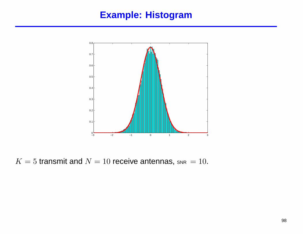
Example: Histogram
−3 −2 −1 0 1 2 30
0.1
0.2
0.3
0.4
0.5
0.6
0.7
0.8
K = 5 transmit and N = 10 receive antennas, SNR = 10.
98

Example: 10%-Outage Capacity ( K = N = 2)
.
. Gaussian approximation
Simulation
Transmitter ( K =2)
Receiver ( N =2)
0
2
4
6
8
10
12
14
0 5 10 15 20 25 30 35 40
SNR (dB)
10%
Out
age
Cap
acity
(bi
ts/s
/Hz)
SNR (dB) Simul. Asympt. 0 0.52 0.50 10 2.28 2.27
99

Example: 10%-Outage Capacity ( K = 4, N = 2)
.
. Gaussian approximation
Simulation
Transmitter ( K =4)
Receiver ( N =2)
0
4
8
12
16
0 5 10 15 20 25 30 35 40
SNR (dB)
10%
Out
age
Cap
acity
(bi
ts/s
/Hz)
100

Summary
• Various wireless communication channels: analysis tackled with the aidof random matrix theory.
• Shannon and η-transforms, motivated by the application of randommatrices to the theory of noisy communication channels.
• Shannon transforms and η-transforms for the asymptotic ESD of severalclasses of random matrices.
• Application of the various findings to the analysis of several wirelesschannel in both ergodic and non-ergodic regime.
• Succinct expressions for the asymptotic performance measures.
• Applicability of these asymptotic results to finite-size communicationsystems.
101
Reference
A. M. Tulino and S. Verdu“Random Matrices and Wireless Communications,”
Foundations and Trends in Communications and Information Theory,vol. 1, no. 1, June 2004.
http://dx.doi.org/10.1561/0100000001
102

Theory of Large Dimensional Random Matrices for Engineers
(Part II)
Jack SilversteinNorth Carolina State University
The 9th International Symposium on Spread Spectrum Techniques and Applications, Manaus, Amazon, Brazil,
August 28-31, 2006

1. Introduction. Let M(R) denote the collection of all sub-
probability distribution functions on R. We say for {FN} ⊂ M(R),
FN converges vaguely to F ∈ M(R) (written FNv−→ F ) if for all
[a, b], a, b continuity points of F , limN→∞ FN{[a, b]} = F{[a, b]}. We
write FND−→ F , when FN , F are probability distribution functions
(equivalent to limN→∞ FN (a) = F (a) for all continuity points a of F ).
For F ∈M(R),
SF (z) ≡∫
1x− z
dF (x), z ∈ C+ ≡ {z ∈ C : =z > 0}
is defined as the Stieltjes transform of F .
1

Properties:
1. SF is an analytic function on C+.
2. =SF (z) > 0.
3. |SF (z)| ≤ 1=z .
4. For continuity points a < b of F
F{[a, b]} =1π
limη→0+
∫ b
a
=SF (ξ + iη)dξ.
5. If, for x0 ∈ R, =SF (x0) ≡ limz∈C+→x0 =SF (z) exists, then F is
differentiable at x0 with value ( 1π )=SF (x0) (Silverstein and Choi
(1995)).
2
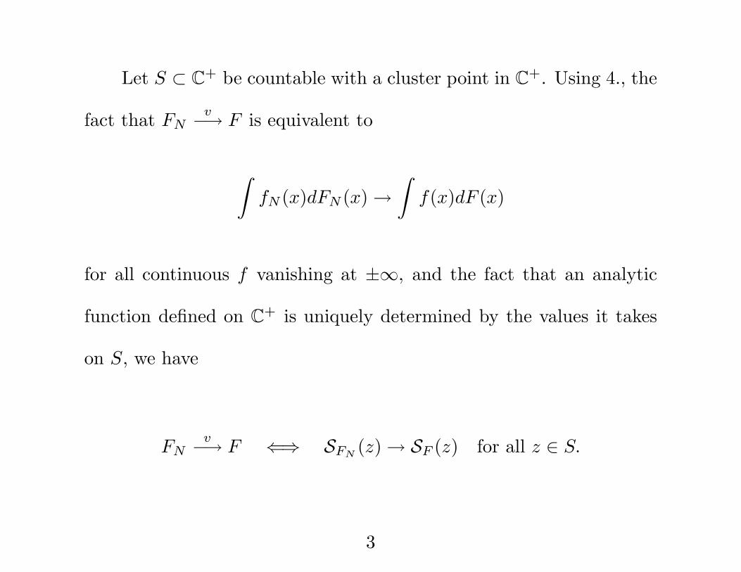
Let S ⊂ C+ be countable with a cluster point in C+. Using 4., the
fact that FNv−→ F is equivalent to
∫fN (x)dFN (x) →
∫f(x)dF (x)
for all continuous f vanishing at ±∞, and the fact that an analytic
function defined on C+ is uniquely determined by the values it takes
on S, we have
FNv−→ F ⇐⇒ SFN
(z) → SF (z) for all z ∈ S.
3

The fundamental connection to random matrices:
For any Hermitian N×N matrix A, we let FA denote the empirical
distribution function, or empirical spectral distribution (ESD), of itseigenvalues:
FA(x) =1N
(number of eigenvalues of A ≤ x).
ThenSFA(z) =
1N
tr (A− zI)−1.
So, if we have a sequence {AN} of Hermitian random matrices, to show,with probability one, FAN
v−→ F for some F ∈M(R), it is equivalentto show for any z ∈ C+
1N
tr (AN − zI)−1 → SF (z) a.s.
For the remainder of the lecture SA will denote SFA .
4

The main goal of this part of the tutorial is to present results
on the limiting ESD of three classes of random matrices. The results
are expressed in terms of limit theorems, involving convergence of the
Stieltjes transforms of the ESD’s. An outline of the proof of the first re-
sult will be given. The proof will clearly indicate the importance of the
Stieltjes transform to limiting spectral behavior. Essential properties
needed in the proof will be emphasized in order to better understand
where randomness comes in and where basic properties of matrices are
used.
5

For each of the theorems, it is assumed that the sequence of random
matrices are defined on a common probability space. They all assume:
For N = 1, 2, . . . X = XN = (XNij ), N × K, XN
ij ∈ C, i.d. for all
N, i, j, independent across i, j for each N , E|X11 1 − EX1
1 1|2 = 1, and
K = K(N) with K/N → β > 0 as N →∞.
Let S = SN = (1/√
N)XN .
6

Theorem 1.1 (Marcenko and Pastur (1967), Silverstein and Bai(1995)). Let T be a K ×K real diagonal random matrix whose ESD
converges almost surely in distribution, as N → ∞ to a nonrandom
limit. Let T denote a random variable with this limiting distribution.
Let W0 be an N ×N Hermitian random matrix with ESD converging,
almost surely, vaguely to a nonrandom distribution W0 with Stieltjes
transform denoted by S0. Assume S, T, and W0 to be independent,
Then the ESD of
W = W0 + STS†
converges vaguely, as N →∞, almost surely to a nonrandom distribu-
tion whose Stieltjes transform, S(·), satisfies for z ∈ C+
(1.1) S(z) = S0
(z − β E
[T
1 + TS(z)
]).
It is the only solution to (1.1) in C+.
7

Theorem 1.2 (Silverstein, in preparation). Define H = CSA,
where C is N × N and A is K ×K, both random. Assume that the
ESD’s of D = CC† and T = AA† converge almost surely in distri-
bution to nonrandom limits, and let D and T denote random variables
distributed, respectively, according to those limits. Assume C, A and
S to be independent. Then the ESD of HH† converges in distribu-
tion, as N → ∞, almost surely to a nonrandom limit whose Stieltjes
transform, S(·), is given for z ∈ C+ by
S(z) = E
1
β D E[
T1+z(z)T
]− z
,
where z(z) satisfies
(1.2) z(z) = E
D
β D E[
T1+z(z)T
]− z
.
z(z) is the only solution to (1.2) in C+.
8
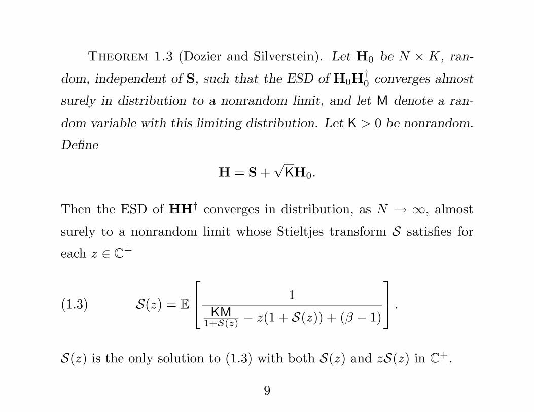
Theorem 1.3 (Dozier and Silverstein). Let H0 be N × K, ran-
dom, independent of S, such that the ESD of H0H†0 converges almost
surely in distribution to a nonrandom limit, and let M denote a ran-
dom variable with this limiting distribution. Let K > 0 be nonrandom.
Define
H = S +√
KH0.
Then the ESD of HH† converges in distribution, as N → ∞, almost
surely to a nonrandom limit whose Stieltjes transform S satisfies for
each z ∈ C+
(1.3) S(z) = E
1
KM1+S(z) − z(1 + S(z)) + (β − 1)
.
S(z) is the only solution to (1.3) with both S(z) and zS(z) in C+.
9
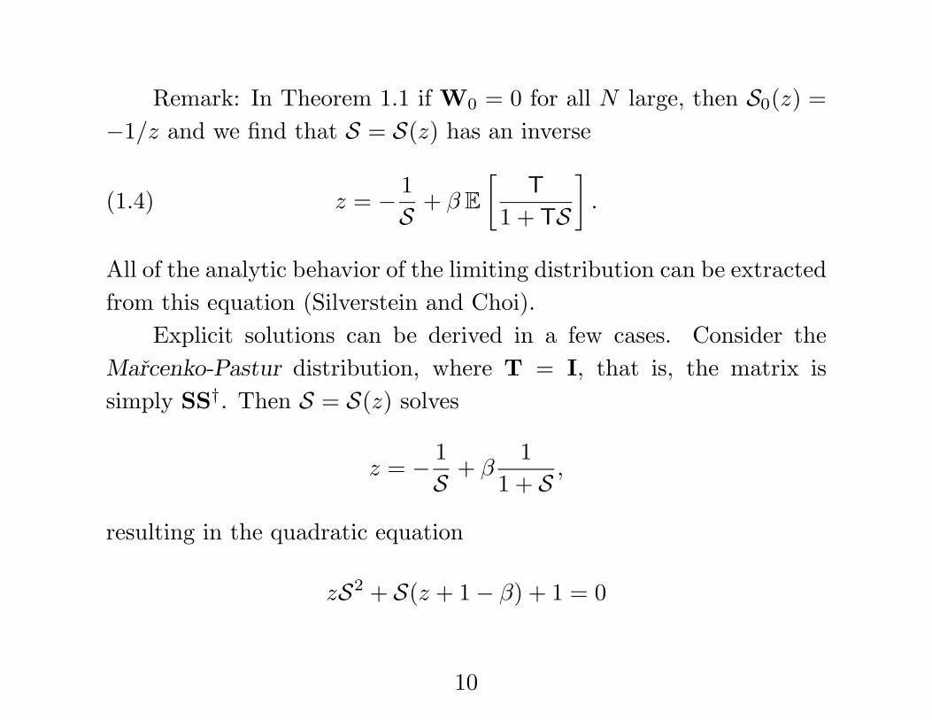
Remark: In Theorem 1.1 if W0 = 0 for all N large, then S0(z) =−1/z and we find that S = S(z) has an inverse
(1.4) z = − 1S + β E
[T
1 + TS]
.
All of the analytic behavior of the limiting distribution can be extractedfrom this equation (Silverstein and Choi).
Explicit solutions can be derived in a few cases. Consider theMarcenko-Pastur distribution, where T = I, that is, the matrix issimply SS†. Then S = S(z) solves
z = − 1S + β
11 + S ,
resulting in the quadratic equation
zS2 + S(z + 1− β) + 1 = 0
10

with solution
S =−(z + 1− β)±√
(z + 1− β)2 − 4z
2z
=−(z + 1− β)±√
z2 − 2z(1 + β) + (1− β)2
2z
=−(z + 1− β)±
√(z − (1−√β)2)(z − (1 +
√β)2)
2z
We see the imaginary part of S goes to zero when z approaches the realline and lies outside the interval [(1−√β)2, (1+
√β)2], so we conclude
from property 5. that for all x 6= 0 the limiting distribution has adensity f given by
f(x) =
{ √(x−(1−
√β)2)((1+
√β)2−x)
2πx x ∈ ((1−√β)2, (1 +√
β)2)0 otherwise.
11

Considering the value of β (the limit of columns to rows) we can
conclude that the limiting distribution has no mass at zero when β ≥ 1,
and has mass 1− β at zero when β < 1.
12

2. Why these theorems are true. We begin with three facts
which account for most of why the limiting results are true, and the
appearance of the limiting equations for the Stieltjes transforms.
Lemma 2.1 For N×N A, q ∈ CN , and t ∈ C with A and A+tqq†
invertible, we have
q†(A + tqq†)−1 =1
1 + tq†A−1qq†A−1
(since q†A−1(A + tqq†) = (1 + tq†A−1q)q†).
Lemma 2.2 For N × N A and B, with B Hermitian, z ∈ C+,
t ∈ R, and q ∈ CN , we have
|tr [(B−zI)−1−(B+tqq†−zI)−1]A| =∣∣∣∣tq†(B− zI)−1A((B− zI)−1q
1 + tq†(B− zI)−1q
∣∣∣∣ ≤ ‖A‖=z
.
13

Proof. The identity follows from Lemma 2.1. We have
∣∣∣∣tq†(B− zI)−1A((B− zI)−1q
1 + tq†(B− zI)−1q
∣∣∣∣ ≤ ‖A‖ |t| ‖(B− zI)−1q‖2|1 + tq†(B− zI)−1q| .
Write B =∑
i λieie∗i , its spectral decomposition. Then
‖(B− zI)−1q‖2 =∑
i
|e†iq|2|λi − z|2
and
|1 + tq†(B− zI)−1q| ≥ |t|=(q†(B− zI)−1q) = |t|=z∑
i
|e†iq|2|λi − z|2 .
14
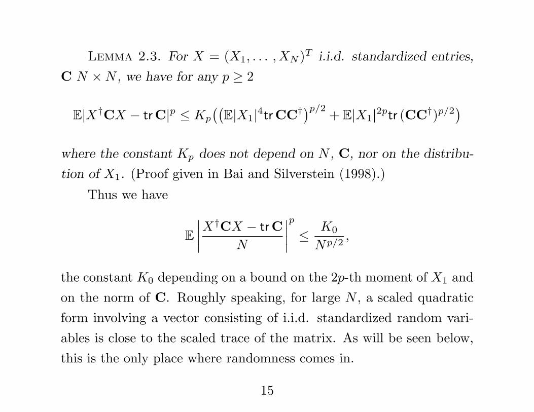
Lemma 2.3. For X = (X1, . . . , XN )T i.i.d. standardized entries,
C N ×N , we have for any p ≥ 2
E|X†CX − trC|p ≤ Kp
((E|X1|4trCC†)p/2 + E|X1|2ptr (CC†)p/2
)where the constant Kp does not depend on N , C, nor on the distribu-
tion of X1. (Proof given in Bai and Silverstein (1998).)
Thus we have
E∣∣∣∣X†CX − trC
N
∣∣∣∣p
≤ K0
Np/2,
the constant K0 depending on a bound on the 2p-th moment of X1 andon the norm of C. Roughly speaking, for large N , a scaled quadraticform involving a vector consisting of i.i.d. standardized random vari-ables is close to the scaled trace of the matrix. As will be seen below,this is the only place where randomness comes in.
15

The first step needed to prove each of the theorems is truncation
and centralization of the elements of X, that is, showing that it is suffi-
cient to prove each result under the assumption the elements have mean
zero, variance 1, and are bounded, for each N , by a rate growing slower
than N (log N is sufficient). These steps will be omitted. Although not
needed for Theorem 1.1, additional truncation of the eigenvalues of D
and T in Theorem 1.2 and HH† in Theorem 1.3, all at a rate slower
than N is also required (again, lnN is sufficient). We are at this stage
able to go through algebraic manipulations, keeping in mind the above
three lemmas, and intuitively derive the equation in Theorem 1.1.
16
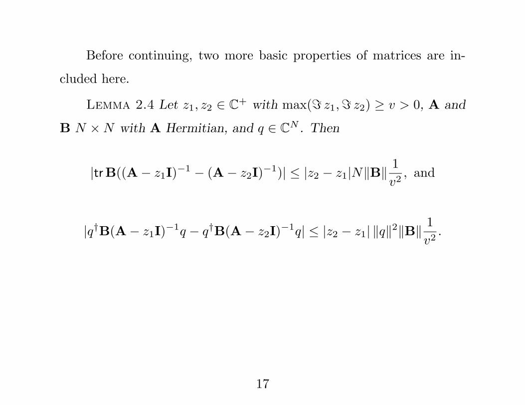
Before continuing, two more basic properties of matrices are in-
cluded here.
Lemma 2.4 Let z1, z2 ∈ C+ with max(= z1,= z2) ≥ v > 0, A and
B N ×N with A Hermitian, and q ∈ CN . Then
|trB((A− z1I)−1 − (A− z2I)−1)| ≤ |z2 − z1|N‖B‖ 1v2
, and
|q†B(A− z1I)−1q − q†B(A− z2I)−1q| ≤ |z2 − z1| ‖q‖2‖B‖ 1v2
.
17
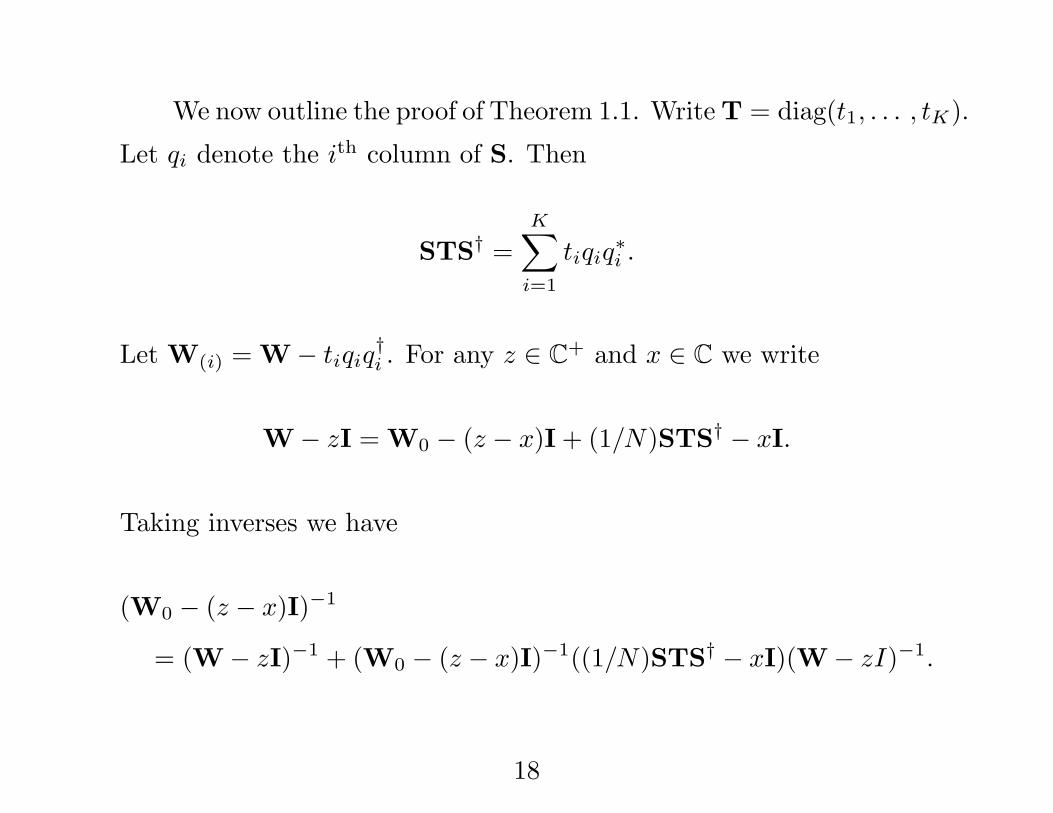
We now outline the proof of Theorem 1.1. Write T = diag(t1, . . . , tK).
Let qi denote the ith column of S. Then
STS† =K∑
i=1
tiqiq∗i .
Let W(i) = W− tiqiq†i . For any z ∈ C+ and x ∈ C we write
W− zI = W0 − (z − x)I + (1/N)STS† − xI.
Taking inverses we have
(W0 − (z − x)I)−1
= (W− zI)−1 + (W0 − (z − x)I)−1((1/N)STS† − xI)(W− zI)−1.
18

Dividing by N , taking traces and using Lemma 2.1 we find
SW0(z−x)−SW(z) = (1/N)tr (W0−(z−x)I)−1
( K∑i=1
tiqiq†i−xI
)(W−zI)−1
= (1/N)n∑
i=1
tiq†i (W(i) − zI)−1(W0 − (z − x)I)−1qi
1 + tiq†i (W(i) − zI)−1qi
− x(1/N)tr (W− zI)−1(W0 − (z − x)I)−1.
Notice when x and qi are independent, Lemmas 2.2, 2.3 give us
q†i (W(i)−zI)−1(W0−(z−x)I)−1qi ≈ (1/N)tr (W−zI)−1(W0−(z−x)I)−1.
19

Letting
x = xN = (1/N)K∑
i=1
ti1 + tiSW(z)
we have
SW0(z − xN )− SW(z) = (1/N)K∑
i=1
ti1 + tiSW(z)
di
where
di =1 + tiSW(z)
1 + tiq†i (W(i) − zI)−1qi
q†i (W(i) − zI)−1(W0 − (z − xN )I)−1qi
− (1/N)tr (W− zI)−1(W0 − (z − xN )I)−1.
In order to use Lemma 2.3, for each i, xN is replaced by
x(i) = (1/N)K∑
j=1
tj1 + tjSW(i)(z)
.
20

Using Lemma 2.3 (p = 6 is sufficient) and the fact that all matrix
inverses encountered are bounded in spectral norm by 1/=z we have
from standard arguments using Boole’s and Markov’s inequalities, and
the Borel-Cantelli lemma, almost surely
(2.1) maxi≤K
max[| ‖qi‖2 − 1|, |q†i (W(i) − zI)−1qi − SW(i)(z)|,
|q†i (W(i)−zI)−1(W0−(z−x(i))I)−1qi−(1/N)tr (W(i)−zI)−1(W0−(z−x(i))I)−1|]
→ 0 as N →∞.
This and Lemma 2.2 imply almost surely
(2.2) maxi≤K
max[|SW(z)−SW(i)(z)|, |SW(z)− q†i (W(i)−zI)−1qi|] → 0,
21

and subsequently, almost surely
(2.3) maxi≤K
max
[∣∣∣∣∣ 1 + tiSW(z)
1 + tiq†i (W(i) − zI)−1qi
− 1
∣∣∣∣∣ , |x− x(i)|]→ 0.
Therefore, from Lemmas 2.2, 2.4, and (2.1) -(2.3), we get maxi≤K di →
0 almost surely, giving us
SW0(z − xN )− SW(z) → 0,
almost surely.
22

On any realization for which the above holds and FW0v−→ W0,
consider any subsequence which SW(z) converges to, say, S, then, on
this subsequence
xN = (K/N)1K
K∑i=1
ti1 + tiSW(z)
→ βE[
T
1 + TS]
Therefore, in the limit we have
S = S0
(z − β E
[T
1 + TS])
,
which is (1.1). Uniqueness gives us, for this realization, SW(z) → S as
N →∞. This event occurs with probability one.
23

3. Proof of uniqueness of (1.1) . For S ∈ C+ satisfying (1.1)
with z ∈ C+ we have
S =∫
1
τ −(z − βE
[T
1 + TS])dW0(τ)
=∫
1
τ −<(z − βE
[T
1 + TS])− i
(=z + βE
[T2=S
|1 + TS|2])dW0(τ)
Therefore
(3.1)
=S =(=z + βE
[T2=S
|1 + TS|2]) ∫
1∣∣∣τ − z + βE[
T1 + TS
]∣∣∣2 dW0(τ)
24

Suppose SSS ∈ C+ also satisfies (1.1). Then(3.2)
S −SSS = β
∫ E[
T1 + TSSS −
T1 + TS
](τ − z + βE
[T
1 + TS]) (
τ − z + βE[
T1 + TSSS
])dW0(τ)
= (S −SSS)βE[
T2
(1 + TS)(1 + TSSS)
]
×∫
1(τ − z + βE
[T
1 + TS]) (
τ − z + βE[
T1 + TSSS
])dW0(τ).
Using Cauchy-Schwarz and (3.1) we have∣∣∣∣βE[
T2
(1 + TS)(1 + TSSS)
]
×∫
1(τ − z + βE
[T
1 + TS]) (
τ − z + βE[
T1 + TSSS
])dW0(τ)
∣∣∣∣∣∣25

≤
βE
[T2
|1 + TS|2] ∫
1∣∣∣τ − z + βE[
T1 + TS
]∣∣∣2 dW0(τ)
1/2
×
βE
[T2
|1 + TSSS|2] ∫
1∣∣∣τ − z + βE[
T1 + TSSS
]∣∣∣2 dW0(τ)
1/2
=
βE
[T2
|1 + TS|2] =S(
=z + βE[
T2=S|1 + TS|2
])
1/2
×
βE
[T2
|1 + TSSS|2] =SSS(
=z + βE[
T2=SSS|1 + TSSS|2
])
1/2
< 1.
Therefore, from (3.2) we must have S = SSS.
26


![Operator-Valued Matrices with Free or Exchangeable Entries€¦ · As applications, we consider random matrices with independent blocks, as in [11], and random matrices in which the](https://img.pdfslide.us/doc/110x75/6059fdb7840fc35b3c17bce1/operator-valued-matrices-with-free-or-exchangeable-entries-as-applications-we-consider.jpg)


![[Madan Lal Mehta] Random Matrices(BookFi-2](https://img.pdfslide.us/doc/110x75/54520983b1af9f7a248b4c20/madan-lal-mehta-random-matricesbookfi-2.jpg)