36

CHAPTER 2

IMPACT OF FWM ON DWDM NETWORKS

2.1 INTRODUCTION

The performance of DWDM systems can be severely degraded by

fiber non-linear effects. Among the consequences of fiber nonlinearity is the

generation of optical inter modulation products, an effect commonly known

as Four Wave Mixing (FWM) (Agarwal 2001). Unfortunately, these FWM

products appear as crosstalk in the transmission bands of the DWDM

tributaries, hence degrading the overall transmission performance of the

system. The FWM efficiency at any particular wavelength is degraded by the

chromatic dispersion of the fiber at that wavelength (Tkach et al 1995).

Dispersion shifted fibers with the WDM signal placed near the zero

dispersion wavelength are normally used to avoid signal distortion due to

dispersion Agarwal (2001). Hence placing the signal wavelengths around the

zero dispersion wavelength of the transmission fiber, the condition of phase-

matching is nearly satisfied and the FWM efficiency gets improved. In the

case of multi-channel systems the FWM generated also gets accumulated

along the length of the fiber, (Lichtman 1991). Thus lower dispersion tends to

enhance the FWM efficiency and hence a compromise has to be made in the

fiber dispersion compensation, (Yu and Mahony 1995).

37

2.2 LIMITATIONS AND PERSPECTIVES OF FWM

FWM is the third order non - linear phenomenon by which two or

more signals propagating simultaneously in a non - linear medium result in

the generation of new signals at new wavelengths. The refractive index

variation induces shifts in the phase of the signals and leads to the generation

of up to N(N-1)2 inter modulation products located at the frequencies fijk = fi ±

fj ± fk , where N denotes the number of original signal wavelengths, (Agarwal

1995). This process is called Four Wave Mixing since four photons are

involved in the interaction. If there are 2 co-propagating waves, then the

number of side bands generated is 2(2 - 1)2 = 2 and this is illustrated in the

Figure 2.1, (Jose Ewerton et al 1997).

2 f1 - f2 2 f2 - f1

f1 f2

Figure 2.1 Four wave mixing with two injected frequencies at f1 and f2

The FWM component centered at frequency fijk = fi + fj - fk where i,

j k, if lies within the receiver bandwidth of existing channels will cause

unwanted interferences. When there are three co - propagating waves, the

newly generated frequency component is f4 = f1 + f2 - f3, if these frequencies

obey the relationship 4 + 3 = 1 + 2. Thus conservation of energy is

satisfied, (Hill et al 1978). In this case, the number of new frequency

components generated is 3 (3 - 1) 2 = 12.

38

Several methods have been proposed in the literature to reduce the

FWM crosstalk penalties. In one approach, a de-multiplexer/multiplexer pair

and fiber delay lines have been used to randomize the phase of the FWM

products, thus increasing the phase mismatch among the various products and

co-propagating DWDM tributaries (Inoue 1993). Alternatively, midway phase

conjugation can be used to cancel out FWM products generated in either half

of a fiber span (Watanabe and Chikama 1994). However, in both cases, the

additional optical devices required to suppress FWM products leads to

increased path loss and implementation costs. Since FWM penalties are

closely related to fiber dispersion characteristics, optimum dispersion maps

could be obtained by the alternative placement of fibers with different

dispersion characteristics to serve as transmission and dispersion

compensating fibers (Nakajima et al 1999) or by using novel optimized fiber

designs (Eiselt 1999). These dispersion maps can however be tailored for best

performance only in a limited part of the transmission window at any

particular time. Chang et al 2000 analyzed the impact of FWM components

due to the channels placed in the unequal spacing of the channels. Forghieri et

al (1995) studied about the improvement in the system performance when the

channels in the WDM systems are unequally spaced.

In WDM systems with equally spaced channels, the newly

generated frequency components fall at the channel frequencies giving rise to

high level of cross talk. For unequally spaced channel scheme, most of the

newly generated frequency components will fall out of the channel

frequencies (Nori Shibata et al 1987). Allocation of unequal spaced channel

systems in WDM light wave systems has been studied by Kwong and Yong

(1995) for suppressing the FWM effect. A Golomb ruler is a set of N integers

such that no two distinct pairs of numbers from the set have the same

difference Atkinson (1986). Thing et al (2004) introduced the fractional

bandwidth allocation algorithm which allows allocating optimal channel

39

spacing with minimum FWM for eight channels ( Thing et al 2003) . Phase

matching of FWM depends on the relative group velocities of the interacting

signals which in turn is determined by the dispersion of the fiber and will be a

function of the signal frequencies and their relative polarizations (Billington

1999). Dispersion management and the relationship between FWM

suppression and Dispersion is very well discussed by Ekaterina et al (1998).

Murakami et al 2002 discussed the impact of higher order dispersion

management in the presence of FWM. The performance of the optical system

can be improved if the channels are allocated around the zero dispersion wave

length region ( Suzuki et al 1999).

In this chapter, the Unequal Spacing Channel (USC) allocation

using Optical Orthogonal Coding (OOC) technique and Genetic algorithm

based channel allocation technique to reduce the FWM effect have been

studied. The number of inter-modulation products falling on the desired

channel for the equal and unequal channel spacing is analyzed. The

performance of OOC based channel allocation towards reducing the effect of

FWM is analyzed for SSMF, NZDSF and DSF fibers. Moreover, the impact

of FWM in SSMF is also studied using a very basic experimental set-up and

by simulations using the OPT Simulation package. To compute the error

probability it is necessary to calculate probability density function of the

received current where the sample space is the set of all possible bit patterns

in all the channels.

2.3 GENETIC ALGORITHM BASED CHANNEL ALLOCATION

In this section, a Genetic Algorithm based WDM channel allocation

is considered with the objective function of reducing FWM. The general steps

involved in a GA based optimization are found in (Haupt 1995). In order to

apply GA based approach in optimizing the WDM channel allocation

40

problem, the chromosomes are defined as an array of parameters to be

optimized. Genes are the basic building block of Genetic algorithm. A gene is

a binary encoding of a parameter. A chromosome is an array of genes. In our

algorithm we predict large list of random chromosomes .The cost function of

each is evaluated and ranked from the most to the least fit with respect to their

cost function. Unacceptable chromosomes are discarded leaving a superior

species - subset of the original list. Genes that survive become parent

chromosomes and reproduce to offset the discarded chromosomes. Mutation

introduces small random changes in a chromosome. Cost functions are

evaluated for the mutated chromosome and the process is repeated.

The algorithm uses binary sequences called genes for channel

allocation. Bit 1 corresponds to the allocation of a channel in that slot and 0

corresponds to the channel not being considered for allocation. In our case,

the cost function is decided by the maximum FWM power falling on the in-

band channels of the WDM system, considering the channel allocation as per

the bit pattern of the corresponding chromosome.

The chromosomes are then ranked from best to worst in terms of

minimizing the maximum FWM power and the ones giving lower value are

preferred and others are discarded and then paired for mating and new

offspring are formed by pair-swapping genetic material. The stopping

criterion is fixed as the maximum average FWM power level acceptable in the

system. The flow chart for the genetic algorithm is shown in Figure 2.2. The

parameters used in the simulation are tabulated in Table 2.1.

41

Table 2.1 Parameters used in the simulation

S.No Parameter Unit SMF

1. Attenuation coefficient (α) dB/km 0.2

2. Chromatic Dispersion (Dc) ps/nm km 16

3. Dispersion slope s/m2 80

4. Nonlinearity coefficient (γ) 1/W km 1.3

5 Effective core area (Aeff) µm2 80

Figure 2.2 Flow chart of the genetic algorithm

The 16 channels selected out of 40 available channels for allocation as a result

of the above optimization is given by their channel numbers as, {1, 2, 4, 6, 10,

12, 14, 17, 20, 22, 27, 29, 30, 37, 38, 40}, ( Ramprasad and Meenakshi 2007).

Establish encoding or decoding of parameters

Generate M random chromosomes

Evaluate cost function of the chromosomes

Rank chromosomes

Discard inferior chromosomes

Remaining chromosomes mate

STOP Mutations

Stopping criteria

No Yes

42

2.4 OPTICAL ORTHOGONAL CODES BASED CHANNEL

ALLOCATION

An Optical Orthogonal Code (OOC) is a family of (0, 1) sequences

with good auto- and cross-correlation properties (Chung et al 1989) i.e., the

autocorrelation of each sequence exhibits the “thumbtack” shape and the cross

correlation between any two sequences remains low throughout. Its study has

been motivated by its application in code division multiple-access scheme in a

fiber optical channel (kitayama et al 1999). The efficiency of four wave

mixing depends on fiber dispersion and channel spacing, (Ekaterina et al

1998). In a Unequal spacing channel USC scheme the signal waves and newly

generated waves have different wavelengths. Since the dispersion varies with

wavelength, the group velocities of the signal waves and generated waves are

different. This destroys the phase matching of the interacting waves and

lowers the efficiency with which power is transferred to newly generated

frequencies

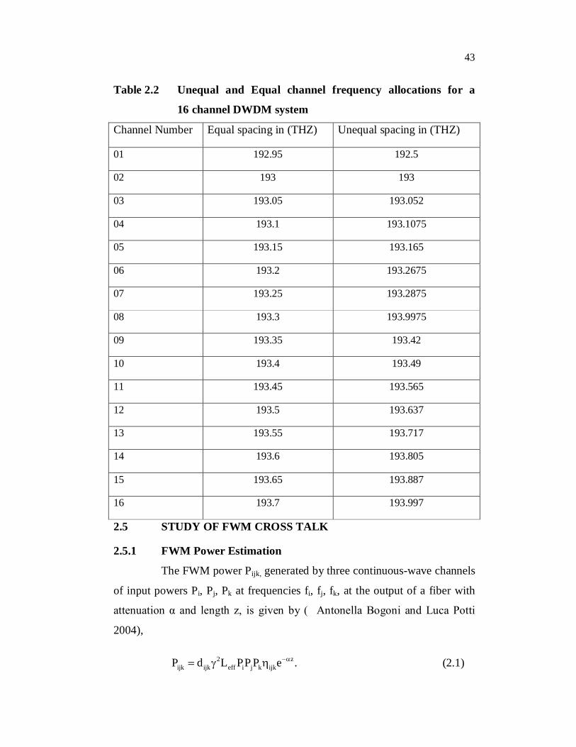
2.4.1 Illustration of a 16 Channel Assignment

A 16 channel intensity modulated direct detection DWDM system

spanning f1-f16 is considered. The bit rate per channel is set at 40 Gbits/s. The

minimum channel spacing of 0.02 THz is selected for ESC and 0.02 THz for

USC. Table 2.2 illustrates Equal and Unequal channel frequency allocations

for a 16 channel DWDM system (Ramprasad and Meenakshi (2006). The

band width expansion factor is approximately equal to 2.

43

Table 2.2 Unequal and Equal channel frequency allocations for a

16 channel DWDM system

Channel Number Equal spacing in (THZ) Unequal spacing in (THZ)

01 192.95 192.5

02 193 193

03 193.05 193.052

04 193.1 193.1075

05 193.15 193.165

06 193.2 193.2675

07 193.25 193.2875

08 193.3 193.9975

09 193.35 193.42

10 193.4 193.49

11 193.45 193.565

12 193.5 193.637

13 193.55 193.717

14 193.6 193.805

15 193.65 193.887

16 193.7 193.997

2.5 STUDY OF FWM CROSS TALK

2.5.1 FWM Power Estimation

The FWM power Pijk, generated by three continuous-wave channels

of input powers Pi, Pj, Pk at frequencies fi, fj, fk, at the output of a fiber with

attenuation α and length z, is given by ( Antonella Bogoni and Luca Potti

2004),

2 zijk ijk eff i j k ijkP d L PP P e . (2.1)

44

where dijk is the degeneracy factor, taking a value of one or two for degenerate

(i = j) and non-degenerate (i ≠ j) terms, respectively; Leff the effective length;

γ the nonlinear coefficient; and ηijk the efficiency.

2

2

eff 0

2 nA

(2.2)

where n2 is the fiber nonlinearity index, λ0 the comb central wavelength and

Aeff the effective core area. ∆βijk represents the phase matching coefficient.

The efficiency ijk and the phase matching coefficient are approximated, for

long enough fiber spans as,

2

ijk 2ijk

(2.3)

ijk c ik jk20

2 c D

(2.4)

where ∆ik and ∆jk are the wavelength spacing between channels i and k, and j

and k, respectively. This approximation is valid for the SMF and NZDSF

fibers in the C-band. In the case of channels arranged on an equally spaced

grid, as the ITU grid, ∆βijk takes the discrete values,

2n c2

0

2 cn D

(2.5)

and hence the efficiency becomes,

ηn = η (∆βn), (2.6)

45

where n = | i-k| | j-k | is the efficiency order, ∆λ is the selected ITU grid

resolution, typically being a multiple of 0.2 nm and is the efficiency of

individual channel.

The number of crosstalk components falling on the desired

channels and the overall number of inter modulation products generated due

to FWM for an Equal spacing channel (ESC) scheme are shown in Figures 2.3

and 2.4. Figure 2.4 shows that there are nearly 3500 inter modulation

frequency components falling on the channel frequency 1.942 *10 14 Hz,

however this is not an allotted channel frequency.Figures 2.5 and 2.6 show

the corresponding results for the USC scheme based on OOCs. It is noted

from the figures that though a large number of inter modulation components

are generated, none of them actually fall on the desired channel frequency.

This implies that though FWM is not eliminated it’s impact on the desired

channels has been removed by the use of OOC based USC scheme. The total

bandwidth occupation for ESC is given by BESC = (n-1) channel spacing

=15*50 GHz =0.75 THz, where n is the number of channels, 16 in this case.

The corresponding bandwidth occupation for USC is BUSC = (193.9975-192.5)

THz = 1.4975 THz. The bandwidth expansion factor BUSC / B ESC = 1.4975 /

0.75 ~ 2.

The 16 channels selected out of 40 available wavelengths for

allocation as a result of optimization using genetic algorithm is given by their

channel numbers as, {1, 2, 4, 6, 10, 12, 14, 17, 20, 22, 27, 29, 30, 37, 38, 40}.

The corresponding FWM power obtained are shown in Figure 2.7. It is

observed from the figure that after optimization and channel allocation,

maximum FWM power is occurring at the 8th and the 9th channels, it’s

strength being -6 dBm. However from Figure 2.5 it is noted that the number

of FWM components falling on the desired channels is zero for OOC based

allocation and hence the FWM power on desired channels is zero. Thus the

impact of FWM crosstalk power on desired channels in a DWDM optical

46

system is found to be less when the channel spacing is unequally allotted

based on Optical Orthogonal Coding technique as compared to the Genetic

algorithm technique, (Ramprasad and Meenakshi 2007) .

Figure 2.8 illustrates the the FWM power versus the power per

channel in mWs. The parameters taken for estimation are as follows: Fiber

length 17.5 km, Nonlinear refractive index 2.68e-20, core effective area 50

m2, frequency allocation = [193.0, 193.1, 193.2, 193.3] THz. This cross talk

power is calculated using the Equations (2.1) to (2.4). It is seen that the FWM

power increases with the increase in the channel power.

Figure 2.3 Number of cross talk components falling on the desired

channels in ESC scheme

47

Figure 2.4 Overall number of inter modulation components generated

due to FWM in ESC scheme

Figure 2.5 Number of cross talk components falling on the desired

channels in USC scheme

48

Figure 2.6 Number of Inter modulation products generated due to

FWM in USC

Figure 2.7 FWM power under optimal allocation using GA

49

EC335 TRANSMISSION LINES AND NETWORKS 3 0 0 100 1. TRANSMISSION LINE THEORY & PARAMETERS : 10

Introduction to different types of transmission lines, Definition of line parameters, the transmission line, - General Solution, Physical Significance of the equations, the infinite line, input impedance, loading of transmission line, waveform distortion, Distortion less transmission line, input and transfer impedance, Reflection phenomena, Line losses, Return loss, reflection loss, insertion loss. 2. THE LINE AT RADIO AND POWER FREQUENCIES: 9

Parameters of open wire line and Coaxial line at high frequencies; Line constants for dissipation less line - voltages and currents on dissipation less line - standing waves and standing wave ratio - input impedance of open and short circuited lines - power and impedance measurement on lines – real and reactive power –Measurement using network analyser. Design consideration for open – wire, resonant line and Coaxial line 3. IMPEDANCE MATCHING AND IMPEDANCE TRANSFORMATION: 9

Reflection losses on unmatched line - Eighth wave line - Quarter wave and half wave line- Exponential line -Tapped Quarter wave line for impedance transformation - single and double stub matching - smith chart and its applications - problem solving using smith chart.

Figure 2.8 FWM noise versus Power per channel

2.5.2 Experimental Study

In a standard single mode fiber, a very low value of crosstalk power

is expected because FWM efficiency at any wavelength is degraded by the

chromatic dispersion at that wavelength. This is experimentally verified using

a partially degenerate FWM set up. The schematic arrangement for this is

shown in Figure 2.9 and the photograph of the same is shown in Figure 2.10.

Figure 2.9 Experimental setup to observe FWM using SMF

Lambda 1

Lambda 2

3 dB coupler OPTICAL

SPECTRUM ANALYSER SMF

50

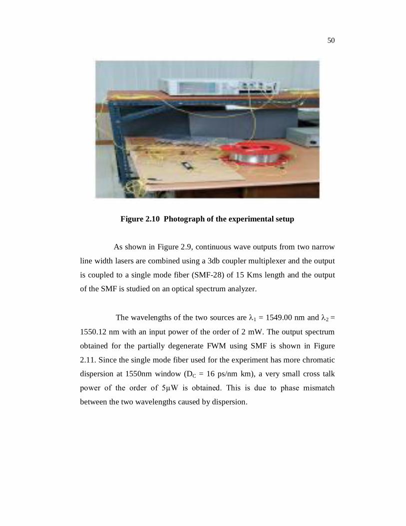
Figure 2.10 Photograph of the experimental setup

As shown in Figure 2.9, continuous wave outputs from two narrow

line width lasers are combined using a 3db coupler multiplexer and the output

is coupled to a single mode fiber (SMF-28) of 15 Kms length and the output

of the SMF is studied on an optical spectrum analyzer.

The wavelengths of the two sources are 1 = 1549.00 nm and 2 =

1550.12 nm with an input power of the order of 2 mW. The output spectrum

obtained for the partially degenerate FWM using SMF is shown in Figure

2.11. Since the single mode fiber used for the experiment has more chromatic

dispersion at 1550nm window (DC = 16 ps/nm km), a very small cross talk

power of the order of 5µW is obtained. This is due to phase mismatch

between the two wavelengths caused by dispersion.

51

Figure 2.11 Output spectrum obtained for the partially degenerate

FWM using SMF of length 5 km

As shown in Figure 2.11 the output spectrum shows FWM power

measured in dBm along the y - axis and input wavelength of operation in the

x-axis. Since there is insufficient vertical magnification of the spectrum

analyzer which is used to measure the power of the output spectrum, a distinct

FWM of stokes and anti-stoke wavelengths is not seen.

2.5.3 Simulation Study

In the preliminary experiment it was seen that in single mode

fibers, a very low value of crosstalk power is generated. However using

dispersion shifted fiber (DSF) and operating with the signals close to or at the

zero dispersion wavelength results in increased phase matching and hence

higher FWM efficiencies (Agrawal 2001). If the power generated in the

sidebands due to FWM is sufficient, these sidebands can further mix, giving

52

rise to multiple sidebands ( Bosco et al 2000). This concept can be used in

the design of a multi-wavelength source for wavelength division multiplexed

systems. Since cost of DSF is very high, it was not possible to verify them by

experiment and therefore a computer simulation is carried out in our work to

observe the FWM products using DSF for 2 channels (partially degenerate

FWM) and 16 channel WDM transmission systems. Computer simulation

allows various scenarios to observe FWM products and to calculate FWM

cross talk power. The simulation begins by creating an electric field for each

channel including laser line-width as a random walk of the phase. The

parameters of the DSF (Cartaxo 1999) used in the simulation set up are shown

in Table 2.3.

Table 2.3 Parameters of the DSF used in the simulation

1. Length 50 km 2. Attenuation Constant 0.25 dB/km 3. Input coupling efficiency 1 dB 4. Output coupling efficiency 0.022dB 5. Group delay constant 49,00,000 ps/km 6. GVD constant 4.5 ps/nm/km 7. Dispersion slope constant 0.072 ps/nm2/km 8. Birefrigence constant 6.25 rad/m 9. Effective area constant 72 micron2

10. Non-linear co-efficient 2.128

Here continuous wave outputs from 2 CW lasers, made to operate

at a wavelength of 1.54 µm and 1.5405 µm are combined using 2x1

multiplexer. The wavelength separation between the 2 sources is 0.5 nm.

Input power is set for both the sources as 8 dBm (6mW). The multiplexed

light output is sent through a 50km long DSF and the output of the DSF is

studied on an optical spectrum analyzer. Similarly the simulation model for a

sixteen channel WDM system is also setup as shown in

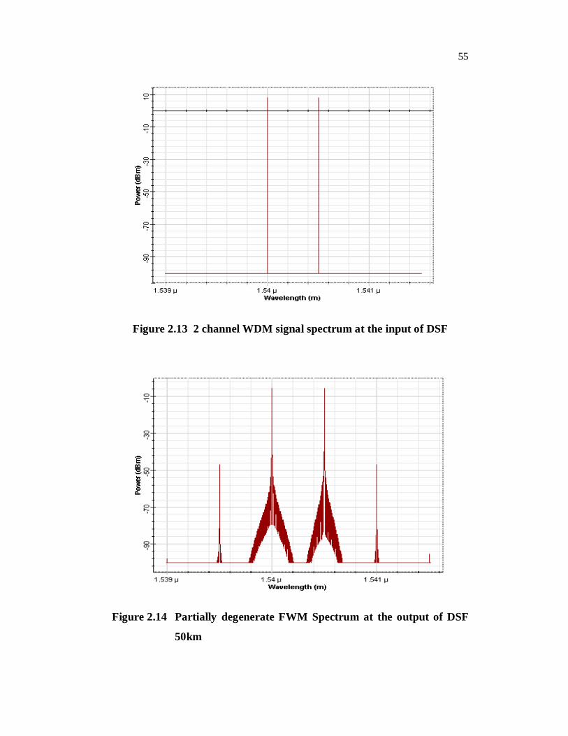
Figures 2.12, to observe in-band FWM products. Figure 2.13 shows the

53

spectrum of signal at the input of the Dispersion Shifted Fiber for the

simulation done for 2 channels WDM and Figure 2.14 shows the spectrum of

signal at the output of the Dispersion Shifted Fiber. It is seen that, the input

signals spectral widths are widened due to their propagation through the fiber.

The partially degenerate FWM components can also be observed with the

separation between new frequency and input frequency being equal to the

separation of the 2 input frequencies. Here partially degenerate FWM means

that f1 is not equal to f2 but they are nearly equal. Similarly the separation

between the new wavelength and input wavelength both on the left hand side

and the right hand side is equal to 0.5 nm. The DSF used has a zero dispersion

wavelength of 1544 nm and a dispersion slope of 0.072 ps/km-nm2. The value

of n2 used is 2.4 10-20 and degeneracy is 3.

The simulation results for the 16 channel WDM transmission

system are shown in Figures 2.15, 2.16 and 2.17. Figure 2.15 shows the

spectrum of signal at the input of the Dispersion Shifted Fiber for the

simulation done for unequally spaced 16 channels WDM and Figure 2.16

shows the spectrum of signal at the output of the Dispersion Shifted Fiber.

54

Figure 2.12 Simulation model for 16 channel WDM

55

Figure 2.13 2 channel WDM signal spectrum at the input of DSF

Figure 2.14 Partially degenerate FWM Spectrum at the output of DSF

50km

56

Figure 2.15 16 unequal channel WDM spectrum at the input of DSF

Figure 2.16 FWM cross talk components in unequal spacing

Pow

er (d

Bm

)

Frequency (Hz)

57

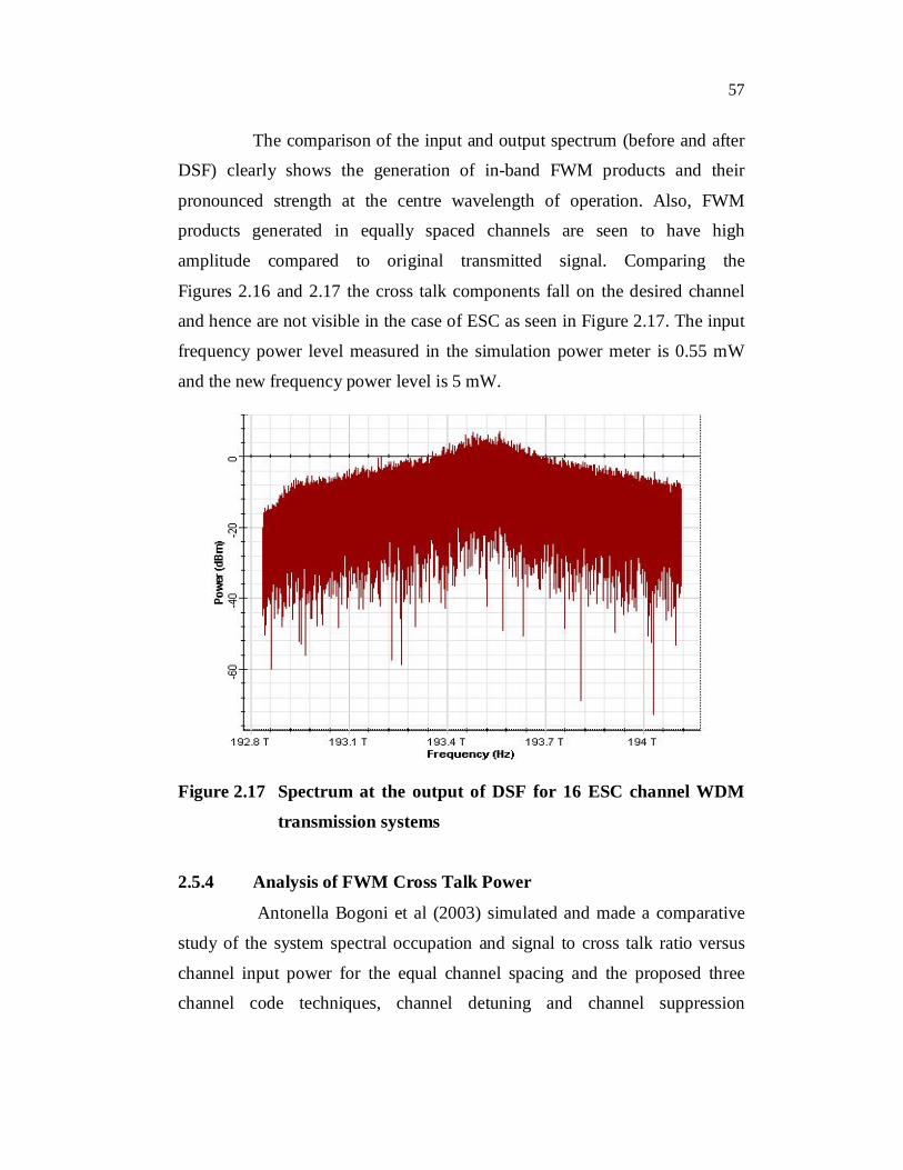
The comparison of the input and output spectrum (before and after

DSF) clearly shows the generation of in-band FWM products and their

pronounced strength at the centre wavelength of operation. Also, FWM

products generated in equally spaced channels are seen to have high

amplitude compared to original transmitted signal. Comparing the

Figures 2.16 and 2.17 the cross talk components fall on the desired channel

and hence are not visible in the case of ESC as seen in Figure 2.17. The input

frequency power level measured in the simulation power meter is 0.55 mW

and the new frequency power level is 5 mW.

Figure 2.17 Spectrum at the output of DSF for 16 ESC channel WDM

transmission systems

2.5.4 Analysis of FWM Cross Talk Power

Antonella Bogoni et al (2003) simulated and made a comparative

study of the system spectral occupation and signal to cross talk ratio versus

channel input power for the equal channel spacing and the proposed three

channel code techniques, channel detuning and channel suppression

58

techniques . Also signal to cross talk ratio has been reported for NZDSF, SM

and DS fibers using Three channel coding (TCC) and Equal spacing channel.

In our model the FWM cross talk generated by multiplexing

channels are examined and its power can be estimated using the expression

for the FWM based on Equation (2.6) (Inoue et al 1994),

6 2p q r L

FWM 4 2 2 20 eff

P P P1024 (D )P en c A

2(mn)M m 1 N n 1

(k) (mj) 00 (mn)

m 1 k 1 n 1 j 1

( i Lexpi exp ( i L 1 expi

(2.6)

Aeff is the effective mode area , PP , Pq , Pr are the input powers of the

sources, M = 5 number of sections, n = 3 is the number of fibers in one

section ,Lo is the length of one fiber ,α is the fiber loss coefficient, n0 is the

refractive index, is phase difference coefficient, c is the light velocity,

D is the degeneracy factor. The parameters taken in the calculations are

L0 = 10 Km, the number of spans N=50, repeater span L = 100 Km, fiber

loss=0.2 db/km, third order nonlinear susceptibility χ=4x10-8esu, the zero

dispersion wavelength=1550nm, Chromatic dispersion (DC) and Dispersion

slope are set corresponding to the fiber type .

The FWM crosstalk power is analyzed for all the three fibers. An

accurate analysis of the four wave mixing impact on DWDM system is

carried out for different types of fibers. Unequally spaced channel allocation

is carried out with the optical spreading code and the performances are

compared for various fiber types. Table 2.4 lists some of the important

parameters of the three primary fiber types, namely, SMF, DSF and NZDSF.

Single mode fiber has more chromatic dispersion and also a high value of

non-linearity coefficient.

59

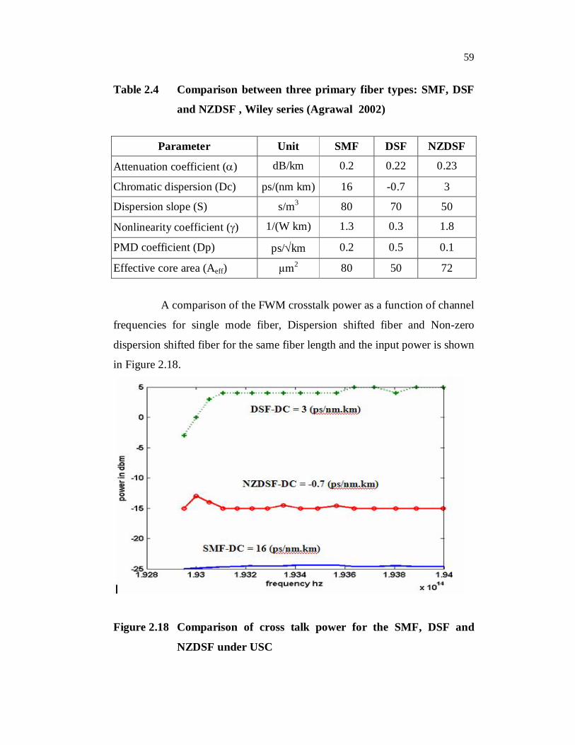
Table 2.4 Comparison between three primary fiber types: SMF, DSF

and NZDSF , Wiley series (Agrawal 2002)

Parameter Unit SMF DSF NZDSF

Attenuation coefficient () dB/km 0.2 0.22 0.23

Chromatic dispersion (Dc) ps/(nm km) 16 -0.7 3

Dispersion slope (S) s/m3 80 70 50

Nonlinearity coefficient () 1/(W km) 1.3 0.3 1.8

PMD coefficient (Dp) ps/km 0.2 0.5 0.1

Effective core area (Aeff) µm2 80 50 72

A comparison of the FWM crosstalk power as a function of channel

frequencies for single mode fiber, Dispersion shifted fiber and Non-zero

dispersion shifted fiber for the same fiber length and the input power is shown

in Figure 2.18.

Figure 2.18 Comparison of cross talk power for the SMF, DSF and

NZDSF under USC

60

The Unequal channel spacing allocated using spreading codes is

considered for all the three fiber transmissions. A comparison of maximum

FWM crosstalk power under the USC scheme for the three fiber types is

shown in Table 2.5. The dispersion shifted fiber has a maximum crosstalk

power of about 2.8 mW and the single mode fiber has about 5µW,

(Ramprasad and Meenakshi 2006).

The Non-zero dispersion shifted fiber occupies a place in between

single mode fiber and dispersion shifted fiber possessing a crosstalk power of

about 0.125mW. The reduced dispersion of Non-zero dispersion shifted fiber

(NZDSF) with less FWM crosstalk power makes this fiber a suitable

candidate for deployment in multi-channel WDM systems.

Table 2.5 Comparison of maximum crosstalk power for SMF, DSF

and NZDSF for USC scheme

Sl. No. Fiber Type Crosstalk Power

1. Single mode fiber 5 µW

2. Dispersion Shifted fiber 2.8 mW

3. Non-Zero Dispersion Shifted fiber 0.125 mW

A plot of FWM efficiency versus ∆βn (phase constant for various

wavelengths) for NZDSF is shown in Figure 2.19. FWM efficiency is plotted

for the discrete values of ∆βn with ∆λ = 0.2 nm and z =100 km. The penalty

induced by FWM is more pronounced if ∆β is too low or Pijk (hence Pi, Pj, or

Pk) exceed a certain threshold level. The phase matching condition (∆β=0) is

easily achieved if the chromatic dispersion of the fiber is low and/or the

frequency spacing between the co-propagating signals is reduced. Hence

FWM efficiency is inversely proportional to dispersion and channel spacing

61

and therefore high FWM efficiency is obtained when the phase mismatch is

low. This affects the design of DWDM systems by limiting transmit power

and number of channels. The pump powers being low, the effects of SPM and

XPM could be neglected ( Song et al 1999).

Figure 2.19 FWM efficiency versus phase matching co-efficient for

NZDSF

2.5.5 FWM Noise Statistics

Performances of an optical transmission system are measured in

terms of the Optical Signal to Noise Ratio (OSNR), the Q factor and the Bit

Error Rate. In optical transmission systems, the optical noise entering the

receiver dominates the electrical noise generated in the receiver. An optical

noise is produced by EDFA and the preamplifier prior to the receiver. Other

parameters that affect the performance are the sampling time and the decision

level used to differentiate between the mark and space levels. The BER is

usually estimated from the probability density function of the sampled

62

electrical currents corresponding to the Mark and the Space state. Monte carlo

simulations are used to obtain histograms of the currents in the Mark and the

Space states where different samples corresponds to different realization of

the random variables in the system.

Considering a sixteen channel WDM in which one of the

multiplexed light wavelengths is selected by an optical filter in the receiver,

the light amplitude E, at the selected signal frequency is given by the

following equation Inoue(1994),

1/ 2 j s 1/ 2 j pqrs s p q r pqr

pqrE B (P ) e B B B (P ) e (2.7)

where Ps and s are the peak power and the phase respectively of the selected

light signal. Pp q r, p q r are the peak power and the phase respectively of

FWM generated from a combination of p, q and r th channels that satisfy p + q

- r = s and Bi = 1 or 0, when the i th channel is Mark or Space, respectively.

The summation term in equation (2.7) accounts for all channel combinations

satisfying p + q – r = s. The channel combinations are further classified into

three categories; (i) the case where all the channels including the selected

channels are different (p ≠ q ≠ r ≠ s), (ii) when p, q and r channels are

different but the r th channel is identical to the selected channel (p ≠ q ≠ r = s)

and (iii) when p and q channels are identical (p = q ≠ r) but are different from

r th channel. These are expressed as,

pqr p q r s p q r s p q r I II III

(2.8)

where summation I, II and III denote summation for p ≠ q ≠ r ≠ s , p ≠ q ≠ r =s

and p = q ≠ r cases, respectively. At the receiver the photocurrent is

proportional to the optical power and hence to |E |2, where E = E(m) or E(s). For

63

large distance L, exp (-αL) << 1. Hence in our analysis we have assumed a

single fiber span without optical amplification and all other receiver noises

assumed negligible. This is justified for high input powers.

The photocurrent obtained from Inoue (1994) for the Mark and

space state at the detector is used for the study of its statistical behavior. In the

current research work, a random simulation to study the nature of FWM noise

is carried out and the pdfs of Im and Is are computed by Monte Carlo

simulations , (Ramprasad and Meenakshi 2006).

The other parameters used for the simulation are fiber length L

=150 km having an EDFA for a span of 75 kms to compensate for the

attenuation of 0.22 dB/km. The power in each channel is set to 10 mW,

minimum channel spacing is taken to be 20 GHz, dispersion slope 0.06

ps/km.nm2, effective core area is 50 µm2, non-linear refractive index is 2.69

10-20 m2/W, number of channels 16, number of spans is 2, allocated

bandwidth is 800 GHz. Figure 2.20 shows the pdf of the mark state receiver

current Im obtained from the random experiments. Similarly Figure 2.21 is

plotted for the space current pdf.

64

1.00E-181.00E-151.00E-121.00E-09

1.00E-061.00E-031.00E+00

-20 -10 0 10 20

mark current ( Im)

pdf

Figure 2.20 pdf of the mark state received current

1E-241E-221E-201E-181E-161E-141E-121E-101E-081E-06

0.00010.01

1

0 40

space current ( Is)

pdf

Figure 2.21 pdf of the space state received current

It is found from the random simulation experiments that the

probability distribution of the mark state current is nearly Gaussian distributed

and the space state current exhibits a pdf that is almost exponential in nature.

65

2.6 SUMMARY

In this chapter, the limitation imposed by FWM components on

DWDM systems has been studied. To summarize, a simple and effective

method to observe new wavelength generation due to partially degenerate

FWM has been shown practically using ordinary single mode silica fiber. A

computer simulation was carried out for different types of fibers for 2 channel

and 16 channel WDM fiber optic transmission system to observe FWM

products under ESC and optical orthogonal code based USC. The comparison

of ESC and USC scheme in terms of FWM generation shows that the

unequally spaced channel scheme applicable for any fiber type allowed the

DWDM system to have almost nil FWM crosstalk power. A comparable

performance with equally spaced channel scheme can be obtained at the cost

of transmission length of the fiber and the bit rate / channel.

An USC allocation based on the Genetic algorithm technique,

which is a powerful mathematical optimization technique, was also carried

and the FWM power generation obtained. The impact of FWM crosstalk

power on DWDM optical systems is found to be less when the channel

spacing is unequally allotted based on Optical orthogonal coding technique as

compared to the Genetic algorithm technique. In addition to this, an analysis

of FWM impact on DWDM optical system is carried out for different types of

fibers and a comparison is made on the generated FWM crosstalk power.

This approach consists in optimizing channel allocation by

considering not only the total in-band FWM crosstalk but also the number of

inter- modulation products falling into the channel band width. The numerical

results which are obtained shows that there is more FWM crosstalk power of

2.8 mW generated for the dispersion shifted fibers which are employed to

reduce the dispersion at the operating wavelength 1550nm, a less crosstalk

66

power of 0.125 mW is generated by the non-zero dispersion shifted fibers

which are currently employed because of their minimum dispersion and loss

at the operating wavelength and a very minimum value of crosstalk power of

5 W has been generated in the case of ordinary single mode silica fibers

because of their high value of dispersion at the operating wavelength.

The statistical behavior of the Four wave mixing noise has been

analyzed and the probability density function for the Mark state (one state)

and Space state (zero state) of the detector current in the multi-channel system

are plotted separately. The FWM noise in the receiver photocurrent of the

DWDM multiplexed systems with N=16 channels is determined and it is

found that the distribution is nearly Gaussian distributed for the Mark state

current and has an exponential decay for Space state current.