2-1

Chapter 2

COST ESTIMATINGMETHODOLOGY

William M. VatavukInnovative Strategies and Economics Group, OAQPSU.S. Environmental Protection AgencyResearch Triangle Park, NC 27711

December 1995

2-2

Contents

2.1 Types of Cost Estimates . . . . . . . . . . . . . . . . . . . . . . . . . . . . . . . . . . . . . . . . . . . . . . 2-4

2.2 Cost Categories Defined . . . . . . . . . . . . . . . . . . . . . . . . . . . . . . . . . . . . . . . . . . . . . . 2-5

2.2.1 Elements of Total Capital Investment . . . . . . . . . . . . . . . . . . . . . . . . . . . . . . 2-6

2.2.2 Elements of Total Annual Cost . . . . . . . . . . . . . . . . . . . . . . . . . . . . . . . . . . . 2-7

2.3 Engineering Economy Concepts . . . . . . . . . . . . . . . . . . . . . . . . . . . . . . . . . . . . . . . 2-10

2.3.1 Time Value of Money . . . . . . . . . . . . . . . . . . . . . . . . . . . . . . . . . . . . . . . . . 2-10

2.3.2 Cash Flow . . . . . . . . . . . . . . . . . . . . . . . . . . . . . . . . . . . . . . . . . . . . . . . . . . 2-10

2.3.3 Annualization and Discounting Methods . . . . . . . . . . . . . . . . . . . . . . . . . . 2-13

2.4 Estimating Procedure . . . . . . . . . . . . . . . . . . . . . . . . . . . . . . . . . . . . . . . . . . . . . . . 2-14

2.4.1 Facility Parameters and Regulatory Options . . . . . . . . . . . . . . . . . . . . . . . . 2-14

2.4.2 Control System Design . . . . . . . . . . . . . . . . . . . . . . . . . . . . . . . . . . . . . . . . 2-15

2.4.3 Sizing the Control System . . . . . . . . . . . . . . . . . . . . . . . . . . . . . . . . . . . . . . 2-16

2.4.4 Estimating Total Capital Investment . . . . . . . . . . . . . . . . . . . . . . . . . . . . . . 2-20

2.4.4.1 General Considerations . . . . . . . . . . . . . . . . . . . . . . . . . . . . . . . . . . 2-20

2.4.4.2 Retrofit Cost Considerations . . . . . . . . . . . . . . . . . . . . . . . . . . . . . . 2-21

2.4.5 Estimating Annual Costs . . . . . . . . . . . . . . . . . . . . . . . . . . . . . . . . . . . . . . . 2-23

2.4.5.1 Raw Materials . . . . . . . . . . . . . . . . . . . . . . . . . . . . . . . . . . . . . . . . . 2-23

2.4.5.2 Operating Labor . . . . . . . . . . . . . . . . . . . . . . . . . . . . . . . . . . . . . . . 2-23

2.4.5.3 Maintenance . . . . . . . . . . . . . . . . . . . . . . . . . . . . . . . . . . . . . . . . . . 2-24

2.4.5.4 Utilities . . . . . . . . . . . . . . . . . . . . . . . . . . . . . . . . . . . . . . . . . . . . . . 2-24

2-3

2.4.5.5 Waste Treatment and Disposal . . . . . . . . . . . . . . . . . . . . . . . . . . . . 2-25

2.4.5.6 Replacement Parts . . . . . . . . . . . . . . . . . . . . . . . . . . . . . . . . . . . . . . 2-25

2.4.5.7 Overhead . . . . . . . . . . . . . . . . . . . . . . . . . . . . . . . . . . . . . . . . . . . . . 2-26

2.4.5.8 Property Taxes, Insurance, and Administrative Charges . . . . . . . . 2-27

2.4.5.9 Capital Recovery . . . . . . . . . . . . . . . . . . . . . . . . . . . . . . . . . . . . . . . 2-27

References . . . . . . . . . . . . . . . . . . . . . . . . . . . . . . . . . . . . . . . . . . . . . . . . . . . . . . . . . . . . . 2-28

2-4

This chapter presents a methodology that will enable the user, having knowledge of the sourcebeing controlled, to produce study-level cost estimates for a control system to control that source.The methodology, which applies to each of the control systems included in this Manual, isgeneral enough to be used with other "add-on" systems as well. Further, the methodology mayalso be applicable to estimating costs of fugitive emission controls and of other non-stackabatement methods.

Before presenting this methodology in detail, we should first discuss the various kinds of costestimates and then define the cost categories and engineering economy concepts employed inmaking the estimates.

2.1 Types of Cost Estimates

As noted above, the costs and estimating methodology in this Manual are directed toward the"study" estimate, of ± 30% accuracy. According to Perry's Chemical Engineer's Handbook, astudy estimate is "… used to estimate the economic feasibility of a project before expendingsignificant funds for piloting, marketing, land surveys, and acquisition … [However] it can beprepared at relatively low cost with minimum data."[1] Specifically, to make a study estimate,the following must be known:

Location of the source within the plant;

Rough sketch of the process flow sheet (i.e., the relative locations of the equipment in the system);

Preliminary sizes of, and material specifications for, the system equipment items;

Approximate sizes and types of construction of any buildings required to house the control system;

Rough estimates of utility requirements (e.g., electricity);

Preliminary flow sheet and specifications for ducting and piping;

Approximate sizes of motors required.[1]

In addition, an estimate of the labor hours required for engineering and drafting is needed, asthe accuracy of an estimate (study or otherwise) is highly dependent on the amount ofengineering work expended on the project.

2-5

There are, however, four other types of estimates, three of which are more accurate than thestudy estimate. These are:[1]

Order-of-magnitude. This estimate provides "a rule-of-thumb procedure applied only torepetitive types of plant installations for which there exists good cost history". Its errorbounds are greater than ± 30%. (However, according to Perry's, "… no limits of accuracycan safely be applied to it.") The sole input required for making this level of estimate isthe control system's capacity (often measured by the maximum volumetric flow rate ofthe gas passing through the system). So-called "six-tenths factor" estimates (not to beconfused with factored estimates) are examples of this type.

Scope or Budget authorization or Preliminary. This estimate, nominally of ± 20%accuracy, requires more detailed knowledge than the study estimate regarding the site, flow sheet, equipment, buildings, etc. In addition, rough specifications for the insulationand instrumentation are also needed.

Project control or Definitive. These estimates, accurate to within ± 10%, require yet moreinformation than the scope estimates, especially concerning the site, equipment, andelectrical requirements.

Firm or Contractor's or Detailed. This is the most accurate (± 5%) of the estimate types,requiring complete drawings, specifications, and site surveys. Further, "[t]ime seldompermits the preparation of such estimates prior to an approval to proceed with theproject."[1]

For the purposes of regulatory development, study estimates have been found to beacceptable, as they represent a compromise between the less accurate order-of-magnitude and themore accurate estimate types. The former are too imprecise to be of much value, while the latterare not only very expensive to make, but require detailed site and process-specific knowledge thatmost Manual users will not have available to them.

2.2 Cost Categories Defined

The names given certain categories of costs and what they contain vary considerably throughoutthe literature. Certain words like "capital cost" can have vastly different meanings, which canoften lead to confusion, even among cost estimators. To avoid this confusion and, at the sametime, provide uniformity in the Manual basic terms are defined in this chapter and will be usedthroughout. The terminology used is adapted from that of the American Association of CostEngineers.[2] Although it has been developed for general use, it is readily adaptable to airpollution control system costing.

2-6

First, two general kinds of costs are estimated, total capital investment (TCI) and total annualcost (TAC). These are discussed below.

2-7

2.2.1 Elements of Total Capital Investment

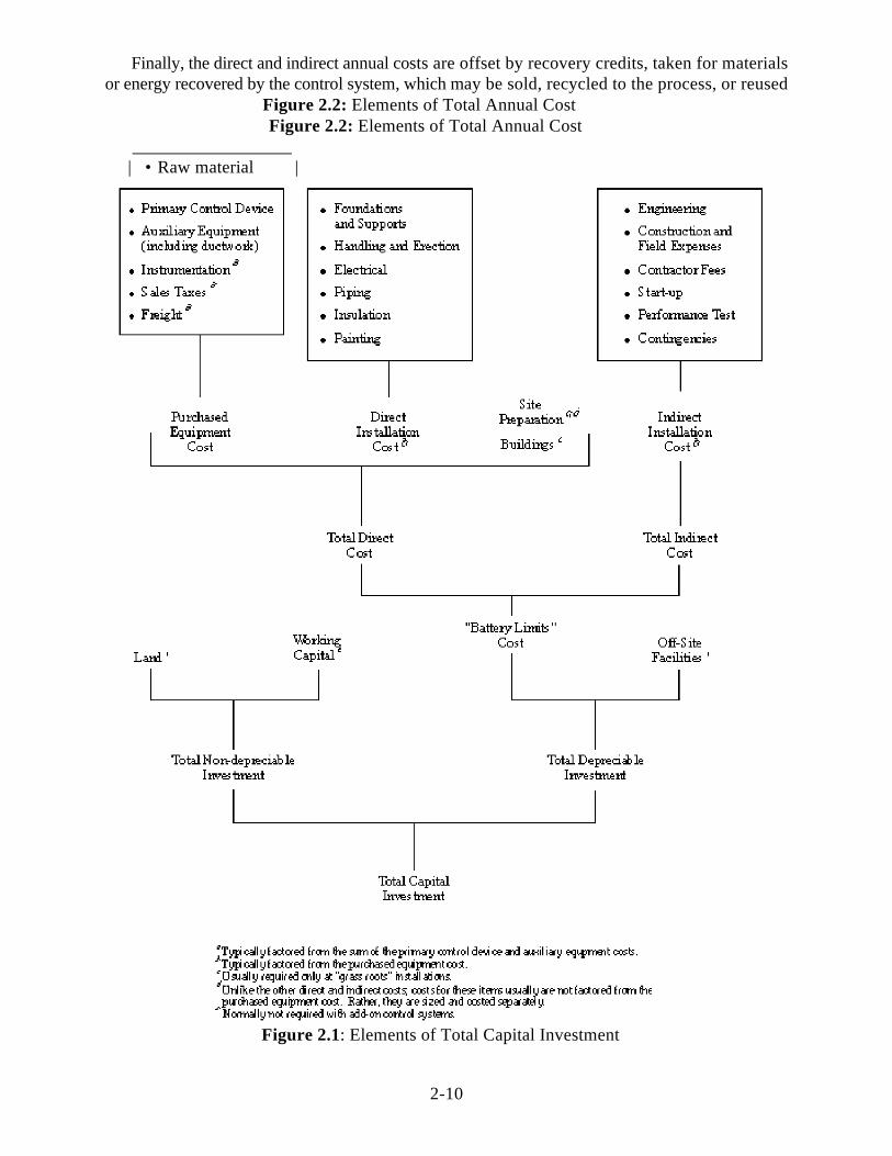
The total capital investment includes all costs required to purchase equipment needed for thecontrol system (termed purchased equipment costs), the costs of labor and materials for installingthat equipment (termed direct installation costs), costs for site preparation and buildings, andcertain other costs which are termed indirect installation costs. The TCI also includes costs forland, working capital, and off-site facilities.

Direct installation costs include costs for foundations and supports, erecting and handling theequipment, electrical work, piping, insulation, and painting. Indirect installation costs includesuch costs as engineering costs; construction and field expenses (i.e., costs for constructionsupervisory personnel, office personnel, rental of temporary offices, etc.); contractor fees (forconstruction and engineering firms involved in the project); start-up and performance test costs(to get the control system running and to verify that it meets performance guarantees); andcontingencies. Contingencies is a catch-all category that covers unforeseen costs that may arise,including (but certainly not limited to)"… possible redesign and modification of equipment,escalation increases in cost of equipment, increases in field labor costs, and delays encounteredin start-up."[2]

These elements of total capital investment are displayed in Figure 2.1. Note that the sum ofthe purchased equipment cost, direct and indirect installation costs, site preparation, and buildingscosts comprises the battery limits estimate. By definition, this is the total estimate "… for aspecific job without regard to required supporting facilities which are assumed to alreadyexist…"[2] at the plant. This would mainly apply to control systems installed in existing plants,though it could also apply to those systems installed in new plants when no special facilities forsupporting the control system (i.e., off-site facilities) would be required.

Where required, these off-site facilities would encompass units to produce steam, electricity,and treated water; laboratory buildings, railroad spurs, roads, and the like. It is unusual, however,for a pollution control system to have one of these units (e.g., a power plant) dedicated to it. Thesystem needs are rarely that great. However, it may be necessary—especially in the case ofcontrol systems installed in new or "grass roots" plants—for extra capacity to be built into the sitegenerating plant to service the system. (A venturi scrubber, which often requires large amountsof electricity, is a good example of this.) It is customary for the utility costs to be charged to theproject as operating costs at a rate which covers both the investment and operating andmaintenance costs for the utility.

As Figure 2.1 shows, there are two other costs which may be included in the total capitalinvestment for a control system. These are working capital and land. The first of these, workingcapital, is a fund set aside to cover the initial costs of fuel, chemicals, and other materials, as wellas labor and maintenance. It usually does not apply to control systems, for the quantities ofutilities, materials, labor, etc., they require are usually small. (An exception might be an oil-firedthermal incinerator, where a small supply (e.g., 30-day) of distillate fuel would have to beavailable during its initial period of operation.)

2-8

Land may also be required. But, since most add-on control systems take up very little space(a quarter-acre or less) this cost would be relatively small. (Certain control systems, such as thoseused for flue gas desulfurization, require larger quantities of land for the process equipment,chemicals storage, and waste disposal.)

Note also in Figure 2.1 that the working capital and land are nondepreciable expenses. Inother words, these costs are "recovered" when the control system reaches the end of its useful life(generally in 10 to 20 years). Conversely, the other capital costs are depreciable, in that theycannot be recovered and are included in the calculation of income tax credits (if any) anddepreciation allowances, whenever income taxes are considered in a cost analysis. (In theManual methodology, however, income taxes are not considered. See Section 2.3.)

Notice that when 100% of the system costs are depreciated, no salvage value is taken for thesystem equipment at the conclusion of its useful life. This is a reasonable assumption for add-oncontrol systems, as most of the equipment, which is designed for a specific source, cannot beused elsewhere without modifications. Even if it were reusable, the cost of disassembling thesystem into its components (i.e., "decommissioning cost") could be as high (or higher) than thesalvage value.

2.2.2 Elements of Total Annual Cost

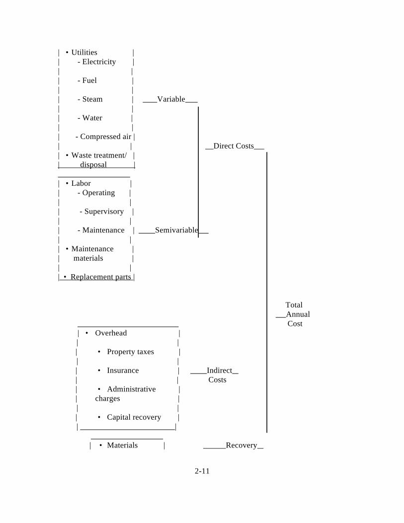
The Total Annual Cost (TAC) for control systems is comprised of three elements: direct costs(DC), indirect costs (IC), and recovery credits (RC),which are related by the following equation:

TAC = DC + IC - RC (2.1)

Clearly, the basis of these costs is one year, as this period allows for seasonal variations inproduction (and emissions generation) and is directly usable in profitability analyses. (SeeSection 2.3.)

Direct costs are those which tend to be proportional or partially proportional to the quantityof exhaust gas processed by the control system per unit time. These include costs for rawmaterials, utilities (steam, electricity, process and cooling water, etc.), waste treatment anddisposal, maintenance materials, replacement parts, and operating, supervisory, and maintenancelabor. Of these direct costs, costs for raw materials, utilities, and waste treatment and disposalare variable, in that they tend to be a direct function of the exhaust flow rate. That is, when theflow rate is at its maximum rate, these costs are highest. Conversely, when the flow rate is zero,so are the costs.

Semivariable direct costs are only partly dependent upon the exhaust flow rate. These includeall kinds of labor, overhead, maintenance materials, and replacement parts. Although these costsare a function of the gas flow rate, they are not linear functions. Even while the control systemis not operating, some of the semivariable costs continue to be incurred.

2-9

Indirect, or "fixed", annual costs are those whose values are totally independent of the exhaustflow rate and, in fact, would be incurred even if the control system were shut down. They includesuch categories as administrative charges, property taxes, insurance, and capital recovery.

2-10

Figure 2.1: Elements of Total Capital Investment

Finally, the direct and indirect annual costs are offset by recovery credits, taken for materialsor energy recovered by the control system, which may be sold, recycled to the process, or reused

Figure 2.2: Elements of Total Annual Cost Figure 2.2: Elements of Total Annual Cost | • Raw material |

2-11

| • Utilities | | - Electricity | | | | - Fuel | | | | - Steam | Variable | | | - Water | | | | - Compressed air | | | Direct Costs | • Waste treatment/ | | disposal | | • Labor | | - Operating | | | | - Supervisory | | | | - Maintenance | Semivariable | | | • Maintenance | | materials | | | | • Replacement parts |

Total Annual

Cost | • Overhead |

| | | • Property taxes |

| | | • Insurance | Indirect | | Costs | • Administrative | | charges |

| | | • Capital recovery |

| |

| • Materials | Recovery

2-12

| | Credits | • Energy |

elsewhere at the site. These credits, in turn, must be offset by the costs necessary for theirprocessing, storage, transportation, and any other steps required to make the recoveredmaterials or energy reusable or resalable. Great care and judgement must be exercised inassigning values to recovery credits, since materials recovered may be of small quantity or ofdoubtful purity, resulting in their having less value than virgin material. Like direct annualcosts, recovery credits are variable, in that their magnitude is directly proportional to theexhaust flow rate. The various annual costs and their interrelationships are displayed inFigure 2.2. A more thorough description of these costs and how they may be estimated isgiven in Section 2.4.

2.3 Engineering Economy Concepts

As mentioned previously, the estimating methodology presented in Section 2.4 rests upon thenotion of the "factored" or "study" estimate. However, there are other concepts central to thecost analyses which must be understood. These are (1) the time value of money, (2) cashflow, and (3) annualization.

2.3.1 Time Value of Money

The time value of money is based on the truism that "…a dollar now is worth more than theprospect of a dollar… at some later date."[3] A measure of this value is the interest rate which"… may be thought of as the return obtainable by the productive investment of capital."[3]

2.3.2 Cash Flow

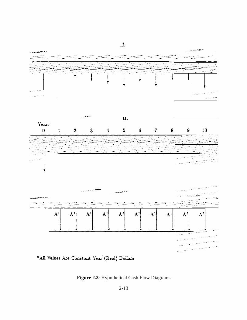
During the lifetime of a project, various kinds of cash expenditures are made and variousincomes are received. The amounts and timing of these expenditures and incomes constitutethe cash flows for the project. In control system costing it is normal to consider expenditures(negative cash flows) and unusual to consider income (positive cash flows), except forproduct or energy recovery income. By the simplifying convention recommended by Grant,Ireson, and Leavenworth[3], each annual expenditure (or payment) is considered to beincurred at the end of the year, even though the payment will probably be made sometimeduring the year in question. (The error introduced by this assumption is minimal, however.) Figure 2.3, which shows three hypothetical cash flow diagrams, illustrates these end-of-yearpayments. In these diagrams, P represents the capital investment, while the A's denote theend-of-year annual payments. Note that in all diagrams, the cash flows are in constant (real)dollars, meaning that they do not reflect the effects of inflation. Also note that in the top

2-13

Figure 2.3: Hypothetical Cash Flow Diagrams

2-14

diagram (I), the annual payments are different for each year. (These represent the controlsystem annual costs (exclusive

CRF i(1 i)n

(1 i) n 1

2-15

(2.3)

of capital recovery) described in Section 2.2.) In reality, these payments would be different,as labor and maintenance requirements, labor and utility costs, etc., would vary from year toyear. A generally upward trend in annual costs would be seen, however.

In diagram II, these fluctuating annual payments have been converted to equal payments. This can be done by calculating the sum of the present values of each of the annual paymentsshown in diagram I and annualizing the total net present value to equivalent equal annualpayments via a capital recovery factor. (See discussion in the following paragraphs and inSection 2.3.3.) Alternatively, it is adequate to choose a value of A equal to the sum of thedirect and indirect annual costs estimated for the first year of the project. This assumption isin keeping with the overall accuracy of study estimates and allows for easier calculations.

Finally, notice diagram III. Here, the annual costs (A ) are again equal, while the capital1

investment (P) is missing. Put simply, P has been incorporated into A , so that A reflects not1 1

only the various annual costs but the investment as well. This was done by introducinganother term, the capital recovery factor (CRF), defined as follows: "when multiplied by apresent debt or investment, [the CRF] gives the uniform end-of-year payment necessary torepay the debt or investment in n years with interest rate i."[3] The product of the CRF andthe investment (P) is the capital recovery cost (CRC):

CRC = CRF x P (2.2)

where

Therefore, A is the sum of A and the CRC, or:l

A = A + CRF x P (2.4)1

In this context, n is the control system economic life, which, as stated above, typicallyvaries from 10 to 20 years. The interest rate (i) used in this Manual is a pretax marginal rateof return on private investment of 7% (annual). This value, which could also be thought of asa "real private rate of return", is used in most of the OAQPS cost analyses and is in keepingwith current OAQPS guidelines and the Office of Management and Budget recommendationfor use in regulatory analyses.[4]

It may be helpful to illustrate the difference between real and nominal interest rates. Themathematical relationship between them is straight forward:[4]

2-16

(1+i ) = (1+i)(1+r) (2.5)n

wherei , i = the annual nominal and real interest rates, respectivelyn

r = the annual inflation rate

Clearly, the real rate does not consider inflation and is in keeping with the expression ofannual costs in constant (i.e., real) dollars.

The above procedure using the pre-tax marginal (or real) rate of return on privateinvestment is the appropriate method for assessing the costs from the perspective of the entityhaving to install the pollution control equipment. For example, costs developed with theabove procedure can appropriately be used for answering questions concerning the marketresponse to regulation like price increases, quantity adjustments, and reduced profitability.

In an idealized economy with perfectly competitive and complete markets, this privatecost and the social cost would be equal. However, in a more realistic economy in whichallocation of resources is distributed by taxes, credit restrictions, and other marketimperfections, the cost to society is different than the private costs for capital expenditures. The costs to society are the relevant costs for use in answering questions about economicefficiency. For example, benefit cost analysis and cost-effectiveness analyses should focus oncost to society, not just the cost to the entity facing additional pollution control costs.

EPA has adopted a new approach, a two-stage approach, to discounting for social costs. This new approach begins with the same capital recovery costs (CRC) described above usingthe same 7% pre-tax marginal rate of return on private investment. The second step of thetwo-stage approach involves "discounting" both direct and indirect annual costs and CRCback to an initial date ("year 0") using a consumption rate of interest of 3%. (See Section2.3.3 for an explanation of the discounting concept.) This results in a relatively higher cost ofcapital from society's perspective than from the perspective of the entity facing additionalcontrol cost. A detailed explanation of this procedure and when it should be employed isbeyond the scope of this document. A fuller explanation is given in draft EPA guidelines [5]. However, it is mentioned here because the CRC and direct and indirect annual costs are inputsto the two-stage procedure and must be sufficiently itemized to allow use in the two-stageprocedure.

2.3.3 Annualization and Discounting Methods

The above method of smoothing out the investment into equal end-of-year payments, istermed the equivalent uniform annual cash flow (EUAC) method.[3] In addition to its inherentsimplicity, this method is very useful when comparing the costs of two or more alternativecontrol systems (i.e., those which are designed to control the same source to an equivalentdegree). In fact, the EUAC's—or simply the total annual costs—of two competing systems

1(1 i) m

2-17

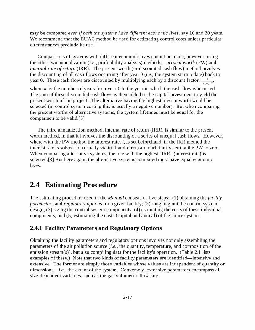
may be compared even if both the systems have different economic lives, say 10 and 20 years. We recommend that the EUAC method be used for estimating control costs unless particularcircumstances preclude its use.

Comparisons of systems with different economic lives cannot be made, however, usingthe other two annualization (i.e., profitability analysis) methods—present worth (PW) andinternal rate of return (IRR). The present worth (or discounted cash flow) method involvesthe discounting of all cash flows occurring after year 0 (i.e., the system startup date) back toyear 0. These cash flows are discounted by multiplying each by a discount factor, ,

where m is the number of years from year 0 to the year in which the cash flow is incurred. The sum of these discounted cash flows is then added to the capital investment to yield thepresent worth of the project. The alternative having the highest present worth would beselected (in control system costing this is usually a negative number). But when comparingthe present worths of alternative systems, the system lifetimes must be equal for thecomparison to be valid.[3]

The third annualization method, internal rate of return (IRR), is similar to the presentworth method, in that it involves the discounting of a series of unequal cash flows. However,where with the PW method the interest rate, i, is set beforehand, in the IRR method theinterest rate is solved for (usually via trial-and-error) after arbitrarily setting the PW to zero. When comparing alternative systems, the one with the highest "IRR" (interest rate) isselected.[3] But here again, the alternative systems compared must have equal economiclives.

2.4 Estimating Procedure

The estimating procedure used in the Manual consists of five steps: (1) obtaining the facilityparameters and regulatory options for a given facility; (2) roughing out the control systemdesign; (3) sizing the control system components; (4) estimating the costs of these individualcomponents; and (5) estimating the costs (capital and annual) of the entire system.

2.4.1 Facility Parameters and Regulatory Options

Obtaining the facility parameters and regulatory options involves not only assembling theparameters of the air pollution source (i.e., the quantity, temperature, and composition of theemission stream(s)), but also compiling data for the facility's operation. (Table 2.1 listsexamples of these.) Note that two kinds of facility parameters are identified—intensive andextensive. The former are simply those variables whose values are independent of quantity ordimensions—i.e., the extent of the system. Conversely, extensive parameters encompass allsize-dependent variables, such as the gas volumetric flow rate.

2-18

Like the facility parameters, the regulatory options are usually specified by others. Theseoptions are ways to achieve a predetermined emission limit. They range from no control tomaximum control technically achievable. The option provided will depend, firstly, onwhether the emission source is a stack (point source), a process leak (process fugitives source)or an unenclosed or partly enclosed area, such as a storage pile (area fugitives source). Stacksare normally controlled by "add-on" devices. As discussed above, this Manual will dealprimarily with these add-on devices. (However, some of these devices can be used to controlprocess fugitives in certain cases, such as a fabric filter used in conjunction with a buildingevacuation

system.) Add-ons are normally used to meet a specified emission level, although in the caseof particulate emissions, they may also be required to meet an opacity level.

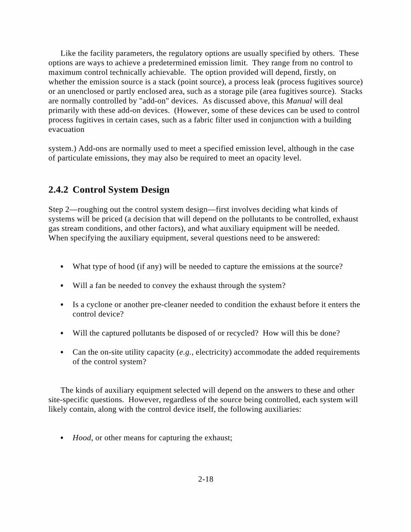
2.4.2 Control System Design

Step 2—roughing out the control system design—first involves deciding what kinds ofsystems will be priced (a decision that will depend on the pollutants to be controlled, exhaustgas stream conditions, and other factors), and what auxiliary equipment will be needed. When specifying the auxiliary equipment, several questions need to be answered:

What type of hood (if any) will be needed to capture the emissions at the source?

Will a fan be needed to convey the exhaust through the system?

Is a cyclone or another pre-cleaner needed to condition the exhaust before it enters the control device?

Will the captured pollutants be disposed of or recycled? How will this be done?

Can the on-site utility capacity (e.g., electricity) accommodate the added requirements of the control system?

The kinds of auxiliary equipment selected will depend on the answers to these and othersite-specific questions. However, regardless of the source being controlled, each system willlikely contain, along with the control device itself, the following auxiliaries:

Hood, or other means for capturing the exhaust;

2-19

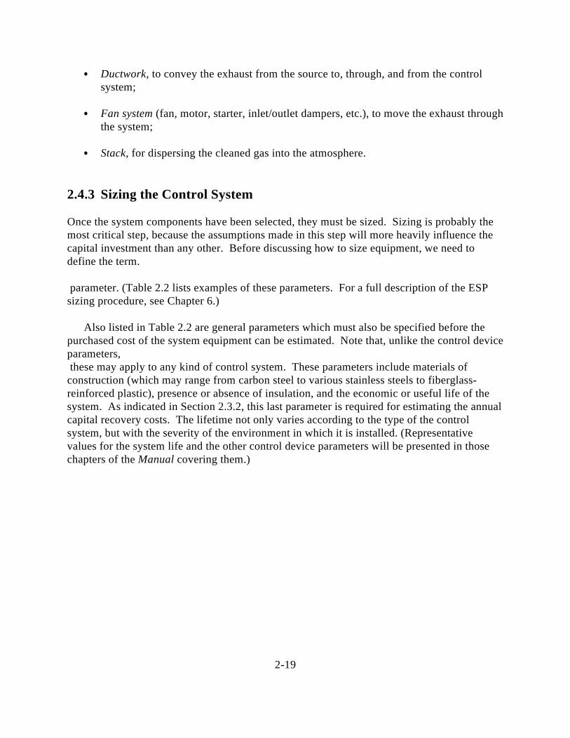
Ductwork, to convey the exhaust from the source to, through, and from the control system;

Fan system (fan, motor, starter, inlet/outlet dampers, etc.), to move the exhaust through the system;

Stack, for dispersing the cleaned gas into the atmosphere.

2.4.3 Sizing the Control System

Once the system components have been selected, they must be sized. Sizing is probably themost critical step, because the assumptions made in this step will more heavily influence thecapital investment than any other. Before discussing how to size equipment, we need todefine the term.

parameter. (Table 2.2 lists examples of these parameters. For a full description of the ESPsizing procedure, see Chapter 6.)

Also listed in Table 2.2 are general parameters which must also be specified before thepurchased cost of the system equipment can be estimated. Note that, unlike the control deviceparameters, these may apply to any kind of control system. These parameters include materials ofconstruction (which may range from carbon steel to various stainless steels to fiberglass-reinforced plastic), presence or absence of insulation, and the economic or useful life of thesystem. As indicated in Section 2.3.2, this last parameter is required for estimating the annualcapital recovery costs. The lifetime not only varies according to the type of the controlsystem, but with the severity of the environment in which it is installed. (Representativevalues for the system life and the other control device parameters will be presented in thosechapters of the Manual covering them.)

2-20

Facility ParametersIntensive

– Facility status (new or existing, location)– Gas characteristics (temperature, pressure, moisture content)– Pollutant concentration(s) and/or particle size distribution

Extensive

– Facility capacity– Facility life– Exhaust gas flow rate– Pollutant emission rate(s)

Regulatory Options

No control

"Add-on" devices

– Emission limits– Opacity limits

Table 2.1: Facility Parameters and Regulatory Options

2-21

2-22

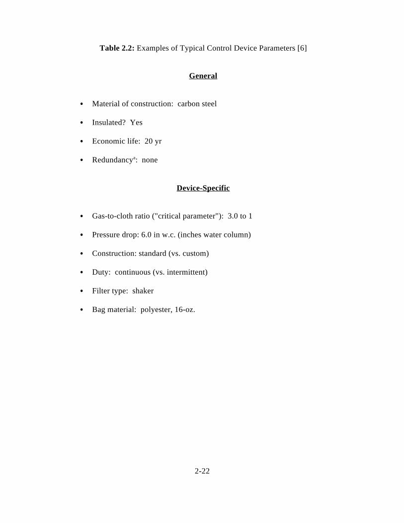
General

Material of construction: carbon steel

Insulated? Yes

Economic life: 20 yr

Redundancy : nonea

Device-Specific

Gas-to-cloth ratio ("critical parameter"): 3.0 to 1

Pressure drop: 6.0 in w.c. (inches water column)

Construction: standard (vs. custom)

Duty: continuous (vs. intermittent)

Filter type: shaker

Bag material: polyester, 16-oz.

Table 2.2: Examples of Typical Control Device Parameters [6]

2-23

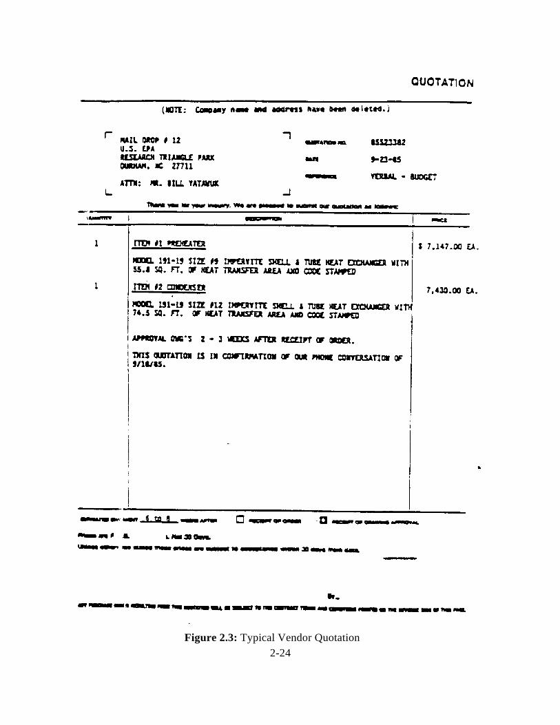
2-24Figure 2.3: Typical Vendor Quotation

2-25

2.4.4 Estimating Total Capital Investment

2.4.4.1 General Considerations

The fourth step is estimating the purchased equipment cost of the control system equipment. These costs are available from this Manual for the most commonly used add-on controldevices and auxiliary equipment. Each type of equipment is covered in a separate chapter.(See Table of Contents.)

Most of these costs, in turn, have been based on data obtained from control equipmentvendors. There are scores of these firms, many of whom fabricate and erect a variety ofcontrol systems. [7] They have current price lists of their equipment, usually indexed bymodel designation. If the items for which costs are requested are fabricated, "off-the-shelf"equipment, then the vendor can provide a written quotation listing their costs, modeldesignations, date of quotation, estimated shipment date, and other information. (See Figure2.4 for a sample quotation.) Moreover, the quote is usually "F.O.B." (free-on-board) thevendor, meaning that no taxes, freight, or other charges are included. However, if the itemsare not off-the-shelf, they must be custom fabricated or, in the case of very large systems,constructed on-site. In such cases, the vendor can still give quotations—but will likely takemuch longer to do so and may even charge for this service, to recoup the labor and overheadexpenses of his estimating department.

As discussed in Section 2.2 in this Manual, the total capital investment is factored fromthe purchased equipment cost, which in turn, is the sum of the base equipment cost (controldevice plus auxiliaries), freight, instrumentation, and sales tax. The values of theseinstallation factors depend on the type of the control system installed and are, therefore, listed in the individualManual chapters dedicated to them.

The costs of freight, instrumentation, and sales tax are calculated differently from thedirect and indirect installation costs. These items are factored also, but from the baseequipment cost (F.O.B. the vendor(s)). But unlike the installation factors, these factors areessentially equal for all control systems. Values for these are as follows:

Retrofit factors for specific applications (coal-fired boiler controls) have been developed. *

See references [9] and [10].

2-26

Cost Range Typical

Freight 0.01 - 0.10 0.05

Sales Tax 0 - 0.08 0.03

Instrumentation 0.05 - 0.30 0.10

The range in freight costs reflects the distance between the vendor and the site. The lowerend is typical of major U.S. metropolitan areas, while the latter would reflect freight chargesto remote locations such as Alaska and Hawaii.[6] The sales tax factors simply reflect therange of local and state tax rates currently in effect in the United States.[8]

The range of instrumentation factors is also quite large. For systems requiring only simplecontinuous or manual control, the lower factor would apply. However, if the control isintermittent and/or requires safety backup instrumentation, the higher end of the range wouldbe applicable.[6] Finally, some "package" control systems (e.g., incinerators covered inChapter 3) have built-in controls, whose cost is included in the base equipment cost. In thosecases, the instrumentation factor to use would, of course, be zero.

2.4.4.2 Retrofit Cost Considerations

The installation factors listed elsewhere in the Manual apply primarily to systems installed innew facilities. These factors must be adjusted whenever a control system is sized for, andinstalled in (i.e., "retrofitted") an existing facility. However, because the size and number ofauxiliaries are usually the same in a retrofit situation, the purchased equipment cost of thecontrol system would probably not be different from the new plant purchased cost. Anexception is the ductwork cost, for in many retrofit situations exceptionally long duct runs arerequired to tie the control system into the existing process.

Each retrofit installation is unique; therefore, no general factors can be developed. *

Nonetheless, some general information can be given concerning the kinds of systemmodifications one might expect in a retrofit:

1. Auxiliaries. Again, the most important component to consider is the ductwork cost. Inaddition, to requiring very long duct runs, some retrofits require extra tees, elbows,dampers, and other fittings.

2-27

2. Handling and Erection. Because of a "tight fit," special care may need to be takenwhen unloading, transporting, and placing the equipment. This cost could increasesignificantly if special means (e.g., helicopters) are needed to get the equipment onroofs or to other inaccessible places.

3. Piping, Insulation, and Painting. Like ductwork, large amounts of piping may beneeded to tie in the control device to sources of process and cooling water, steam, etc. Of course, the more piping and ductwork required, the more insulation and paintingwill be needed.

4. Site Preparation. Unlike the other categories, this cost may actually decrease, formost of this work would have been done when the original facility was built.

5. Off-Site Facilities. Conceivably, retrofit costs for this category could be the largest. For example, if the control system requires large amounts of electricity (e.g., a venturiscrubber), the source's power plant may not be able to service it. In such cases, thesource would have to purchase the additional power from a public utility, expand itspower plant, or build another one. In any case, the cost of electricity supplied to thatcontrol system would likely be higher than if the system were installed in a new sourcewhere adequate provision for its electrical needs would have been made.

6. Engineering. Designing a control system to fit into an existing plant normally requiresextra engineering, especially when the system is exceptionally large, heavy, or utility-consumptive. For the same reasons, extra supervision may be needed when theinstallation work is being done.

7. Lost Production. This cost is incurred whenever a retrofit control system cannot betied into the process during normally scheduled maintenance periods. Then, part or allof the process may have to be temporarily shut down. The net revenue (i.e., grossrevenue minus the direct costs of generating it) lost during this shutdown period is abonafide retrofit expense.

8. Contingency. Due to the uncertain nature of many retrofit estimates, the contingency(i.e., uncertainty) factor in the estimate should be increased. From the above points, itis apparent that some or most of these installation costs would increase in a retrofitsituation.However,there may be other cases where the retrofitted installation costwould be less than the cost of installing the system in a new plant. This could occurwhen one control device, say an ESP, is being replaced by a more efficient unit—abaghouse, for example. The ductwork, stack, and other auxiliaries for the ESP mightbe adequate for the new system, as perhaps would be the support facilities (powerplant, etc.).

L2L1

V2V1

y

2-28

(2.6)

2.4.5 Estimating Annual Costs

Determining the total annual cost is the last step in the estimating procedure. As mentioned inSection 2.2 the TAC is comprised of three components—direct and indirect annual costs andrecovery credits. Unlike the installation costs, which are factored from the purchasedequipment cost, annual cost items are usually computed from known data on the system sizeand operating mode, as well as from the facility and control device parameters.

Following is a more detailed discussion of the items comprising the total annual cost.(Values/factors for these costs are also given in the chapters for the individual devices.)

2.4.5.1 Raw Materials

Raw materials are generally not required with control systems. Exceptions would bechemicals used in gas absorbers or venturi scrubbers as absorbents or to neutralize acidicexhaust gases (e.g., hydrochloric acid). Chemicals may also be required to treat wastewaterdischarged by scrubbers or absorbers before releasing it to surface waters. But, these costsare only considered when a wastewater treatment system is exclusively dedicated to thecontrol system. In most cases, a pro-rata waste treatment charge is applied. (See alsodiscussion below on Waste Treatment and Disposal.)

Quantities of chemicals required are calculated via material balances, with an extra 10 to20% added for miscellaneous losses. Costs for chemicals are available from the ChemicalMarketing Reporter and similar publications.

2.4.5.2 Operating Labor

The amount of labor required for a system depends on its size, complexity, level ofautomation, and operating mode (i.e., batch or continuous). The labor is usually figured on anhours-per-shift basis. As a rule, though, data showing explicit correlations between the laborrequirement and capacity are hard to obtain. One correlation found in the literature islogarithmic:[11]

where

L , L = labor requirements for systems 1 and 21 2

V , V = capacities of systems 1 and 2 (as measured by the gas flow rate, for1 2

instance)

2-29

y = 0.2 to 0.25 (typically)

The exponent in Equation 2.6 can vary considerably, however. Conversely, in manycases, the amount of operator labor required for a system will be approximately the sameregardless of its size.

A certain amount must be added to operating labor to cover supervisory requirements. Fifteen per cent of the operating labor requirement is representative.[12]

To obtain the annual labor cost, multiply the operating and supervisory laborrequirements(labor-hr/operating-hr) by the respective wage rates (in $/labor-hr) and thesystem operating factor (number of hours per year the system is in operation). The wage ratesalso vary widely, depending upon the source category, geographical location, etc. These dataare tabulated and periodically updated by the U.S. Department of Labor, Bureau of LaborStatistics, in its Monthly Labor Review and in other publications. Finally, note that these arebase labor rates, which do not include payroll and plant overhead. (See Overhead discussionbelow.)

2.4.5.3 Maintenance

Maintenance labor is calculated in the same way as operating labor and is influenced by thesame variables. The maintenance labor rate, however, is normally higher than the operatinglabor rate, mainly because more skilled personnel are required. A 10% wage rate premium istypical.[12]

Further, there are expenses for maintenance materials—oil, other lubricants, duct tape,etc., and a host of small tools. Costs for these items can be figured individually, but sincethey are normally so small, they are usually factored from the maintenance labor. Reference[11] suggests a factor of 100% of the maintenance labor to cover the maintenance materialscost.

2.4.5.4 Utilities

This cost category covers many different items, ranging from electricity to compressed air. Of these, only electricity is common to all control devices, where fuel oil and natural gas aregenerally used only by incinerators; water and water treatment, by venturi scrubbers,quenchers, and spray chambers; steam, by carbon adsorbers; and compressed air, by pulse-jetfabric filters.

Techniques and factors for estimating utility costs for specific devices are presented intheir respective sections. However, because nearly every system requires a fan to convey theexhaust gases to and through it, a general expression for computing the fan electricity cost(C ) is given here:[6]e

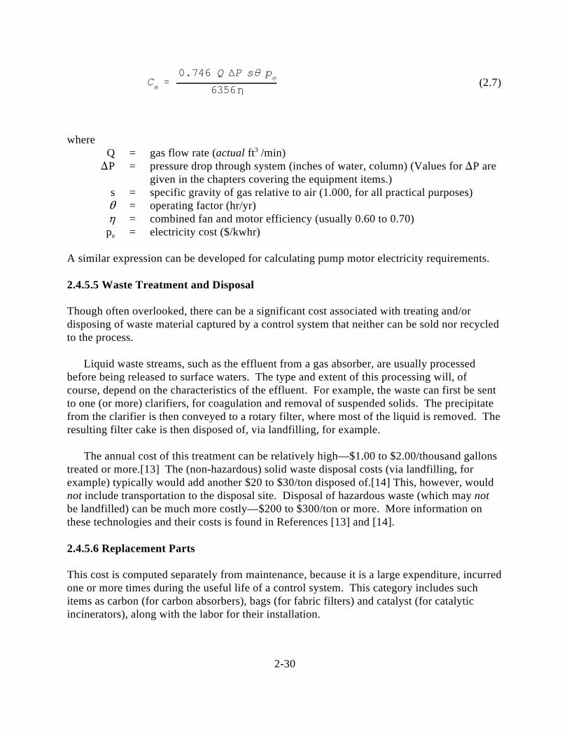
Ce0.746 Q P s pe

6356

2-30

(2.7)

whereQ = gas flow rate (actual ft /min)3

P = pressure drop through system (inches of water, column) (Values for P aregiven in the chapters covering the equipment items.)

s = specific gravity of gas relative to air (1.000, for all practical purposes)= operating factor (hr/yr)= combined fan and motor efficiency (usually 0.60 to 0.70)

p = electricity cost ($/kwhr)e

A similar expression can be developed for calculating pump motor electricity requirements.

2.4.5.5 Waste Treatment and Disposal

Though often overlooked, there can be a significant cost associated with treating and/ordisposing of waste material captured by a control system that neither can be sold nor recycledto the process.

Liquid waste streams, such as the effluent from a gas absorber, are usually processedbefore being released to surface waters. The type and extent of this processing will, ofcourse, depend on the characteristics of the effluent. For example, the waste can first be sentto one (or more) clarifiers, for coagulation and removal of suspended solids. The precipitatefrom the clarifier is then conveyed to a rotary filter, where most of the liquid is removed. Theresulting filter cake is then disposed of, via landfilling, for example.

The annual cost of this treatment can be relatively high—$1.00 to $2.00/thousand gallonstreated or more.[13] The (non-hazardous) solid waste disposal costs (via landfilling, forexample) typically would add another $20 to $30/ton disposed of.[14] This, however, wouldnot include transportation to the disposal site. Disposal of hazardous waste (which may notbe landfilled) can be much more costly—$200 to $300/ton or more. More information onthese technologies and their costs is found in References [13] and [14].

2.4.5.6 Replacement Parts

This cost is computed separately from maintenance, because it is a large expenditure, incurredone or more times during the useful life of a control system. This category includes suchitems as carbon (for carbon absorbers), bags (for fabric filters) and catalyst (for catalyticincinerators), along with the labor for their installation.

2-31

The annual cost of the replacement materials is a function of the initial parts cost, the partsreplacement labor cost, the life of the parts, and the interest rate, as follows:

CRC = (C + C ) CRF (2.8)p p pl p

whereCRC = capital recovery cost of replacement parts ($/yr)p

C = initial cost of replacement parts, including sales taxes and freight ($)p

C = cost of parts-replacement labor ($)pl

CRF = capital recovery factor for replacement parts (defined in Section 2.3).p

In the Manual methodology, replacement parts are treated the same as any otherinvestment, in that they are also considered an expenditure that must be amortized over acertain period. Also, the useful life of the parts (typically 2 to 5 years) is generally less thanthe useful life of the rest of the control system.

Replacement-part labor will vary, depending upon the amount of the material, itsworkability, accessibility of the control device, and other factors.

2.4.5.7 Overhead

This cost is easy to calculate, but often difficult to comprehend. Much of the confusionsurrounding overhead is due to the many different ways it is computed and to the severalcosts it includes, some of which may appear to be duplicative.

There are, generally, two categories of overhead, payroll and plant. Payroll overheadincludes expenses directly associated with operating, supervisory, and maintenance labor,such as: workmen's compensation, Social Security and pension fund contributions, vacations,group insurance, and other fringe benefits. Some of these are fixed costs (i.e., they must bepaid regardless of how many hours per year an employee works). Payroll overhead istraditionally computed as a percentage of the total annual labor cost (operating, supervisory,and maintenance).

Conversely, plant (or "factory") overhead accounts for expenses not necessarily tied to theoperation and maintenance of the control system, including: plant protection, controllaboratories, employee amenities, plant lighting, parking areas, and landscaping. Someestimators compute plant overhead by taking a percentage of all labor plus maintenancematerials [11], while others factor it from the total labor costs alone.[2]

For study estimates, it is sufficiently accurate to combine payroll and plant overhead into asingle indirect cost. This is done in this Manual. Also, overhead is factored from the sum ofall labor (operating, supervisory, and maintenance) plus maintenance materials, the approach

CRCs CRFs [TCI (Cp Cpl)]

2-32

(2.9)

recommended in reference [11]. The factors recommended therein range from 50 to 70% [11]An average value of 60% is used in this Manual.

2.4.5.8 Property Taxes, Insurance, and Administrative Charges

These three indirect operating costs are factored from the system total capital investment, andtypically comprise 1, 1, and 2% of it, respectively. Property taxes and insurance are self-explanatory. Administrative charges covers sales, research and development, accounting, andother home office expenses. (It should not be confused with plant overhead, however.) Forsimplicity, the three items are usually combined into a single, 4% factor. This value,incidentally, is standard in all OAQPS cost analyses.

2.4.5.9 Capital Recovery

As discussed in Section 2.3, the annualization method used in the Manual is the equivalentuniform annualized cost method. Recall that the cornerstone of this method is the capitalrecovery factor which, when multiplied by the total capital investment, yields the capitalrecovery cost. (See Equation 2.2.)

However, whenever there are parts in the control system that must be replaced before theend of its useful life, Equation 2.2 must be adjusted, to avoid double-counting.

That is:

whereCRC = capital recovery cost for control system ($/yr)s

TCI = total capital investment for entire system ($)CRF = capital recovery factor for control system.s

The term (C + C ) accounts for the cost of those parts (including sales taxes and freight) thatp pl

would be replaced during the useful life of the control system and the labor for replacingthem. Clearly, CRF and CRF will not be equal unless the control system and replacements p

part lives are equal.

2-33

References

[1] Perry, Robert H., and Chilton, Cecil H., Perry's Chemical Engineers' Handbook (FifthEdition), McGraw-Hill, New York, 1973, pp. 25-12 to 25-16.

[2] Humphries, K. K. and Katell, S., Basic Cost Engineering, Marcel Dekker, New York,1981, pp. 17-33.

[3] Grant, E.L., Ireson, W.G., and Leavenworth, R.S., Principles of Engineering Economy,Sixth Edition, John Wiley & Sons, New York, 1976.

[4] CEIS (OAQPS) Cost Guidance Memo #2: "Implementing OMB Circular A-94:Guidelines and Discount Rates for Benefit Cost Analysis of Federal Programs," March18, 1993.

[5] Scheraga, Joel D., Draft of "Supplemental Guidelines on Discounting in the Preparationof Regulatory Impact Analyses", Office of Policy, Planning and Evaluation, U.S. EPA,March 31, 1989.

[6] Vatavuk, W.M. and Neveril, R.B., "Estimating Costs of Air-Pollution ControlSystems—Part I: Parameters for Sizing Systems," Chemical Engineering, October 6,1980, pp. 165-168.

[7] Pollution Equipment News 1996 Buyer's Guide, Rimbach Publishing, Pittsburgh, 1996.

[8] Internal Revenue Service, Form 1040, 1985.

[9] Shattuck, D.M., et al., Retrofit FGD Cost-Estimating Guidelines. Electric PowerResearch Institute, Palo Alto, CA (CS-3696, Research Project 1610-1), October 1984.

[10] Kaplan, N., et al., "Retrofit Costs of SO and NO Control at 200 U.S. Coal-Fired Power2 x

Plants," Pittsburgh Coal Conference, 1990.

[11] Peters, M.S. and Timmerhaus, K.D., Plant Design and Economics for ChemicalEngineers (Third Edition), McGraw-Hill, New York, 1980.

[12] Vatavuk, W.M. and Neveril, R.B., "Estimating Costs of Air Pollution ControlSystems—Part II: Factors for Estimating Capital and Operating Costs," ChemicalEngineering, November 3, 1980, pp. 157-162.

[13] Vatavuk, W.M. and Neveril, R.B., "Estimating Costs of Air-Pollution ControlSystems—Part XVII: Particle Emissions Control," Chemical Engineering, April 2, 1984,pp. 97-99.

2-34

[14] The RCRA Risk-Cost Analysis Model, U.S. Environmental Protection Agency, Office ofSolid Waste, January 13, 1984.