Embed Size (px)
Citation preview
Chapter 2
Controlled power operation of
12-pulse converter
.
2.1 Introduction
Many large industrial loads such as used in Steel Plants, Mining etc. need converters
(MW rating) feeding DC motor drives controlling to and fro motion of the mechanical
load. Under such drive environment there are wide fluctuations in the Var demand by the
converter. Those apart, frequent harmonic related problems are also encountered. Passive
filters have been considered good for harmonic current and displacement power factor
compensation. They also are capable of drawing fixed lead Var at fundamental frequency.
When there is a variation of the Var demand by the non-linear loads connected at point
of common coupling (PCC), as in the case of a phase controlled converter feeding DC
motor drive, the passive filters may either over compensate or under compensate reactive
power. Thus the power system continues to be affected by the fluctuations in Var demand
of the load[3].
In the past, many researchers have suggested various Var control techniques using
multiple passive filters, while operating with thyristorized non-linear loads. One such
method is the use of Thyristor switched filter (TSF). By switching on or off the TSF, the
compensator can dynamically adjust reactive power compensation according to the Var
demands of the phase controlled rectifier system.
42
Chapter 2. Controlled power operation ... 43
Among several other methods for converter power factor improvement is asymmetrical
firing control for a 12-pulse converter system where in two 6-pulse converters operate in
cascade In reduced Var operation mode, each 6-pulse converter is fired symmetrically.
But the two converters are controlled as asymmetrical groups. Superconducting magnetic
energy storage systems are getting increasing interest in applications of power flow sta-
bilization and control in the transmission network level. This trend is mainly supported
by the rising integration of large scale wind energy power plants into the high-power util-
ity system and by major features of SMES units. Due to arbitrary variations of wind
speed, Load fluctuation is occurred. So minimization of fluctuation is essential for power
system security. 12 pulse converter has the certain freedom in choosing active & Reac-
tive power. By utilizing the reactive power modulation capacity of the converter, the
inductor-converter unit of function as a static VAR controller using a switched capacitor
bank, while acting as a load frequency stabilizer at the same time. The converter is a
voltage source converter with a controller.
2.2 Operation of 12-pulse converter
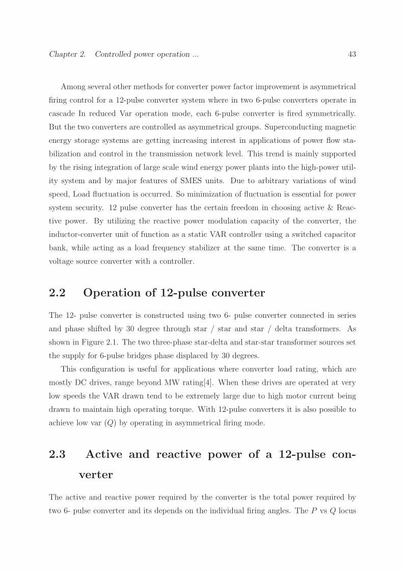
The 12- pulse converter is constructed using two 6- pulse converter connected in series
and phase shifted by 30 degree through star / star and star / delta transformers. As
shown in Figure 2.1. The two three-phase star-delta and star-star transformer sources set
the supply for 6-pulse bridges phase displaced by 30 degrees.
This configuration is useful for applications where converter load rating, which are
mostly DC drives, range beyond MW rating[4]. When these drives are operated at very
low speeds the VAR drawn tend to be extremely large due to high motor current being
drawn to maintain high operating torque. With 12-pulse converters it is also possible to
achieve low var (Q) by operating in asymmetrical firing mode.
2.3 Active and reactive power of a 12-pulse con-
verter
The active and reactive power required by the converter is the total power required by
two 6- pulse converter and its depends on the individual firing angles. The P vs Q locus
Chapter 2. Controlled power operation ... 44
Figure 2.1: 12 pulse converter
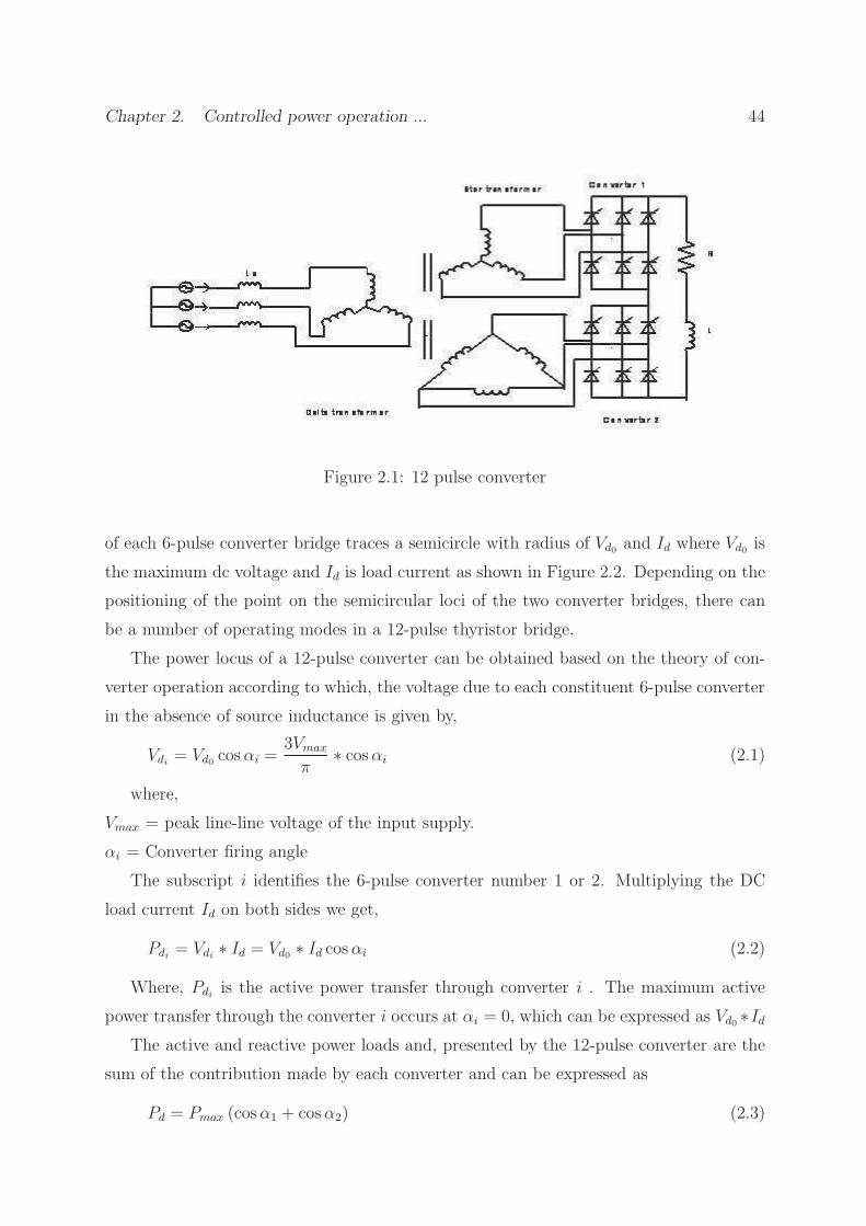
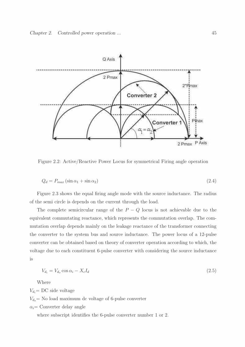
of each 6-pulse converter bridge traces a semicircle with radius of Vd0 and Id where Vd0 is
the maximum dc voltage and Id is load current as shown in Figure 2.2. Depending on the
positioning of the point on the semicircular loci of the two converter bridges, there can
be a number of operating modes in a 12-pulse thyristor bridge.
The power locus of a 12-pulse converter can be obtained based on the theory of con-
verter operation according to which, the voltage due to each constituent 6-pulse converter
in the absence of source inductance is given by,
Vdi= Vd0 cosαi =
3Vmax
π∗ cosαi (2.1)
where,
Vmax = peak line-line voltage of the input supply.
αi = Converter firing angle
The subscript i identifies the 6-pulse converter number 1 or 2. Multiplying the DC
load current Id on both sides we get,
Pdi= Vdi
∗ Id = Vd0 ∗ Id cosαi (2.2)
Where, Pdiis the active power transfer through converter i . The maximum active
power transfer through the converter i occurs at αi = 0, which can be expressed as Vd0 ∗IdThe active and reactive power loads and, presented by the 12-pulse converter are the
sum of the contribution made by each converter and can be expressed as
Pd = Pmax (cosα1 + cosα2) (2.3)
Chapter 2. Controlled power operation ... 45
Figure 2.2: Active/Reactive Power Locus for symmetrical Firing angle operation
Qd = Pmax (sinα1 + sinα2) (2.4)
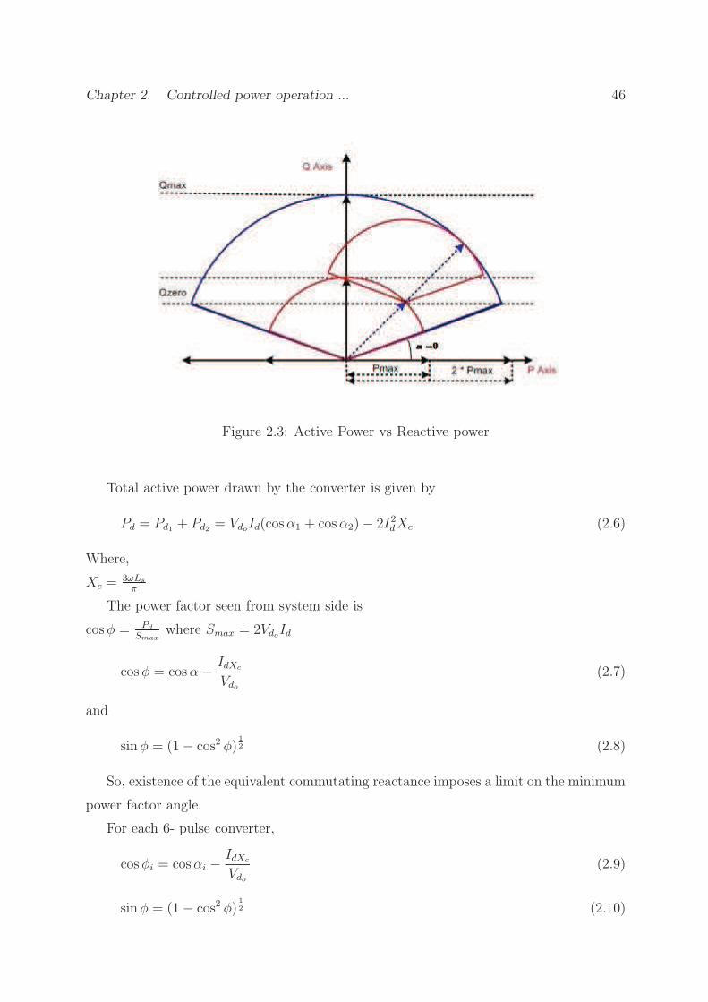
Figure 2.3 shows the equal firing angle mode with the source inductance. The radius
of the semi circle is depends on the current through the load.
The complete semicircular range of the P − Q locus is not achievable due to the
equivalent commutating reactance, which represents the commutation overlap. The com-
mutation overlap depends mainly on the leakage reactance of the transformer connecting
the converter to the system bus and source inductance. The power locus of a 12-pulse
converter can be obtained based on theory of converter operation according to which, the
voltage due to each constituent 6-pulse converter with considering the source inductance
is
Vdi= Vdo cosαi −XcId (2.5)
Where
Vdi= DC side voltage
Vdo= No load maximum dc voltage of 6-pulse converter
αi= Converter delay angle
where subscript identifies the 6-pulse converter number 1 or 2.
Chapter 2. Controlled power operation ... 46
Figure 2.3: Active Power vs Reactive power
Total active power drawn by the converter is given by
Pd = Pd1 + Pd2 = VdoId(cosα1 + cosα2)− 2I2dXc (2.6)
Where,
Xc =3ωLs
π
The power factor seen from system side is
cosφ = Pd
Smaxwhere Smax = 2VdoId
cosφ = cosα−IdXc
Vdo
(2.7)
and
sinφ = (1− cos2 φ)1
2 (2.8)
So, existence of the equivalent commutating reactance imposes a limit on the minimum
power factor angle.
For each 6- pulse converter,
cosφi = cosαi −IdXc
Vdo
(2.9)
sinφ = (1− cos2 φ)1
2 (2.10)
Chapter 2. Controlled power operation ... 47
In the case of equal α mode of converter control
α1 = α2 = α
Pd = 2VdId cosα− 2I2dXc (2.11)
At any point on the P-Q locus, for a given Pd, reactive power Qd is expressed as
Qd = Qd1 +Qd2 where Qd1 , Qd2 are the reactive power drawn by each converter
Theoretically, the converter can be operated over the full 1800 range of delay an-
gle. But because of the effect of the source inductance, its operation is limited. The
commutation angle is given by
µ = cos−1[
cosα−2ωωsId√2VLL
]
(2.12)
Theoretically, the converter can be operated over the full 1800 range of delay angle.
However, the line commutated converters have to be operated between theα + µ to end-
stop. The end stop is defied as the maximum firing angle that can be applied to the
converter so that the converter can be operated without commutation failure, beyond
these limit, risk of commutation failure. Figure 2.3 shows the variation with simultaneous
variation both converter firing angles, the variation of active power and reactive power.
The center is also shifting from zero as the source inductance is increased. And also the
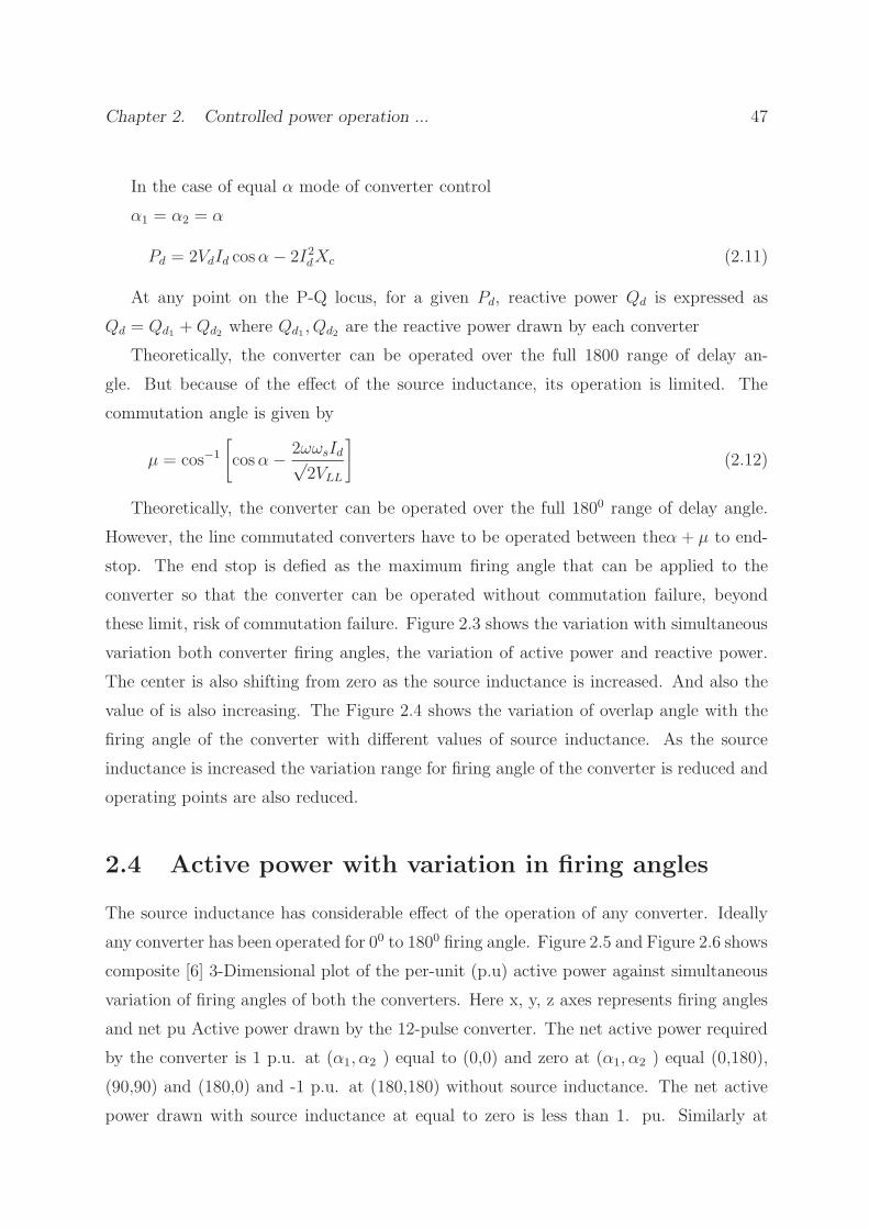
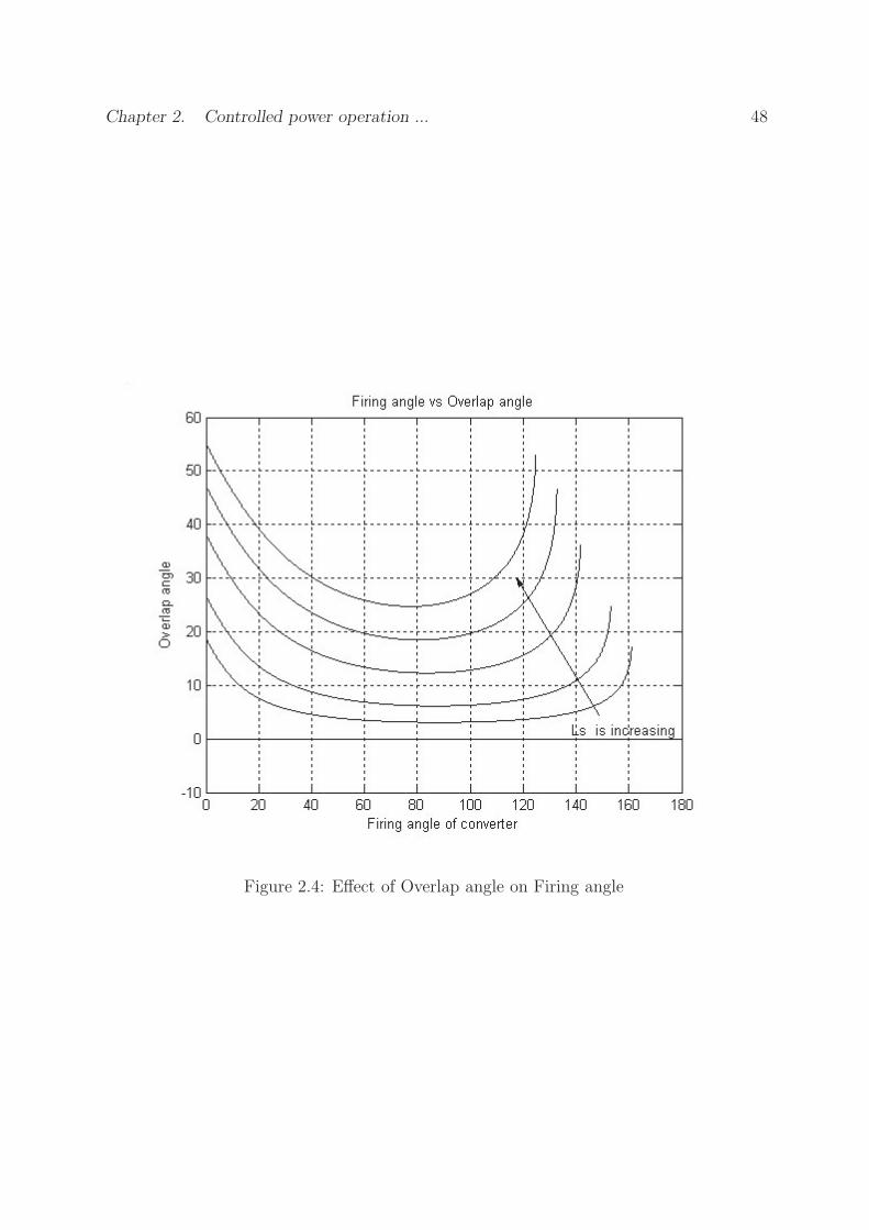
value of is also increasing. The Figure 2.4 shows the variation of overlap angle with the
firing angle of the converter with different values of source inductance. As the source
inductance is increased the variation range for firing angle of the converter is reduced and
operating points are also reduced.
2.4 Active power with variation in firing angles
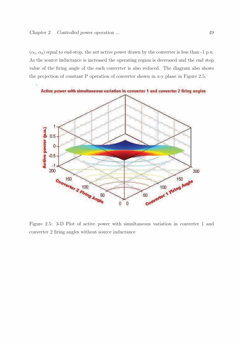
The source inductance has considerable effect of the operation of any converter. Ideally
any converter has been operated for 00 to 1800 firing angle. Figure 2.5 and Figure 2.6 shows
composite [6] 3-Dimensional plot of the per-unit (p.u) active power against simultaneous
variation of firing angles of both the converters. Here x, y, z axes represents firing angles
and net pu Active power drawn by the 12-pulse converter. The net active power required
by the converter is 1 p.u. at (α1, α2 ) equal to (0,0) and zero at (α1, α2 ) equal (0,180),
(90,90) and (180,0) and -1 p.u. at (180,180) without source inductance. The net active
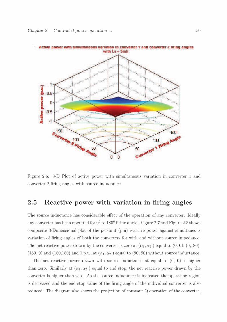
power drawn with source inductance at equal to zero is less than 1. pu. Similarly at
Chapter 2. Controlled power operation ... 48
Figure 2.4: Effect of Overlap angle on Firing angle
Chapter 2. Controlled power operation ... 49
(α1, α2) equal to end-stop, the net active power drawn by the converter is less than -1 p.u.
As the source inductance is increased the operating region is decreased and the end stop
value of the firing angle of the each converter is also reduced. The diagram also shows
the projection of constant P operation of converter shown in x-y plane in Figure 2.5.
Figure 2.5: 3-D Plot of active power with simultaneous variation in converter 1 and
converter 2 firing angles without source inductance
Chapter 2. Controlled power operation ... 50
Figure 2.6: 3-D Plot of active power with simultaneous variation in converter 1 and
converter 2 firing angles with source inductance
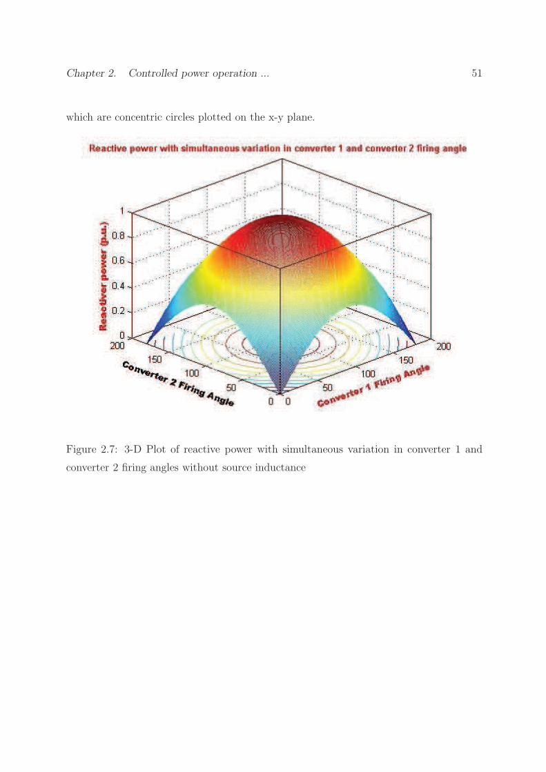
2.5 Reactive power with variation in firing angles
The source inductance has considerable effect of the operation of any converter. Ideally
any converter has been operated for 00 to 1800 firing angle. Figure 2.7 and Figure 2.8 shows
composite 3-Dimensional plot of the per-unit (p.u) reactive power against simultaneous
variation of firing angles of both the converters for with and without source impedance.
The net reactive power drawn by the converter is zero at (α1, α2 ) equal to (0, 0), (0,180),
(180, 0) and (180,180) and 1 p.u. at (α1, α2 ) equal to (90, 90) without source inductance.
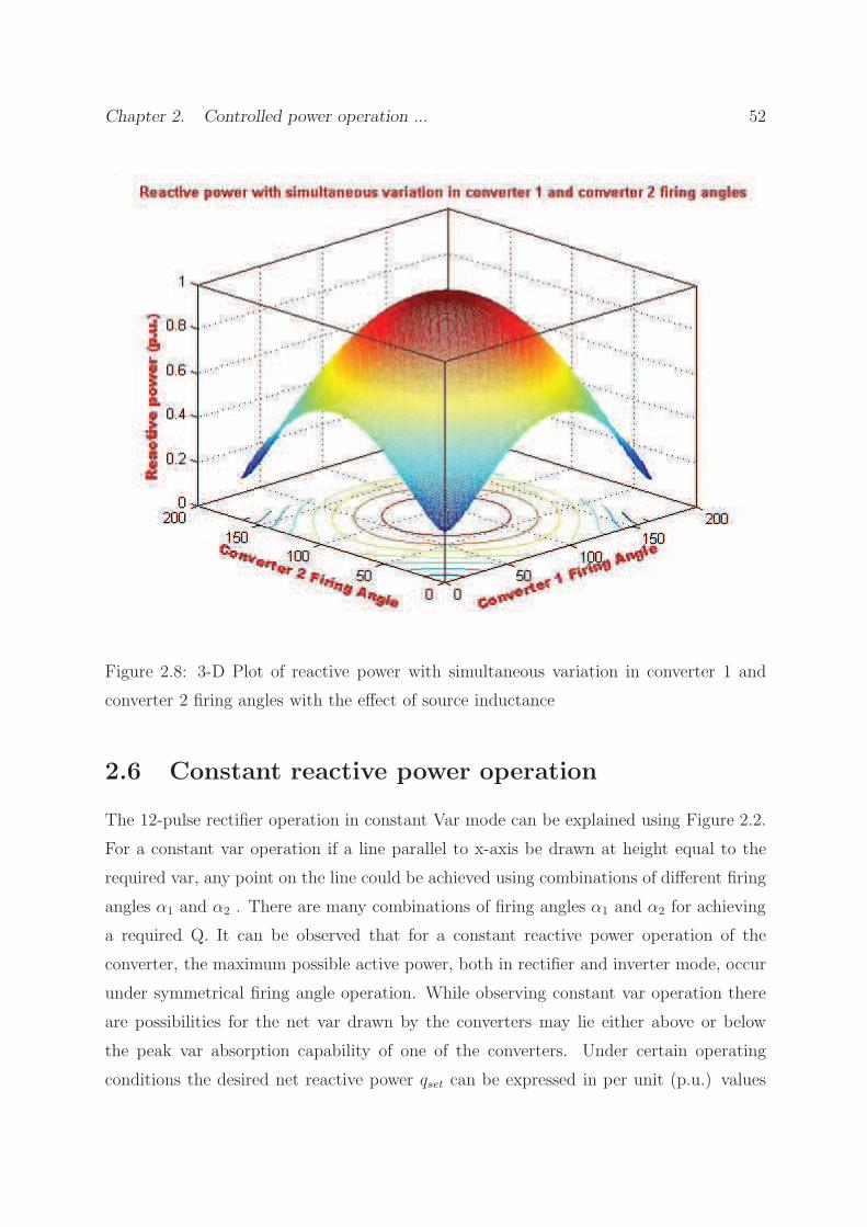
. The net reactive power drawn with source inductance at equal to (0, 0) is higher
than zero. Similarly at (α1, α2 ) equal to end stop, the net reactive power drawn by the
converter is higher than zero. As the source inductance is increased the operating region
is decreased and the end stop value of the firing angle of the individual converter is also
reduced. The diagram also shows the projection of constant Q operation of the converter,
Chapter 2. Controlled power operation ... 51
which are concentric circles plotted on the x-y plane.
Figure 2.7: 3-D Plot of reactive power with simultaneous variation in converter 1 and
converter 2 firing angles without source inductance
Chapter 2. Controlled power operation ... 52
Figure 2.8: 3-D Plot of reactive power with simultaneous variation in converter 1 and
converter 2 firing angles with the effect of source inductance
2.6 Constant reactive power operation
The 12-pulse rectifier operation in constant Var mode can be explained using Figure 2.2.
For a constant var operation if a line parallel to x-axis be drawn at height equal to the
required var, any point on the line could be achieved using combinations of different firing
angles α1 and α2 . There are many combinations of firing angles α1 and α2 for achieving
a required Q. It can be observed that for a constant reactive power operation of the
converter, the maximum possible active power, both in rectifier and inverter mode, occur
under symmetrical firing angle operation. While observing constant var operation there
are possibilities for the net var drawn by the converters may lie either above or below
the peak var absorption capability of one of the converters. Under certain operating
conditions the desired net reactive power qset can be expressed in per unit (p.u.) values
Chapter 2. Controlled power operation ... 53
as sum of the reactive power drawn by constituent converters.
qset(p.u.) = (sinφ1 + sinφ2) ∗ 0.5 (2.13)
At zero firing angle of the both converter the reactive power is given by,
qzero(p.u.) =√
XcId
Vdo
qmax(p.u.) = Smax
qmid(p.u.) = (qmax(p.u.) + qzero(p.u.)) ∗ 0.5 (2.14)
The operation of the 12-pulse converter under this mode can be categorized in two cases.
Case(a) qset ≥ qmid
In this case, there is a minimum firing angle at which each of the converters must work
in order to maintain a constant var. As shown in Figure 2.9, the minimum firing angle
at which one converter will operate will occur when the other converter operates at firing
angle α + µ=90. Thus the minimum firing angle at which each of the converters should
operate are given as under:
q1 =
√
√
√
√1−(
cosα1 −XcId
Smax
)2
(2.15)
q2 = qset − q1
q2 =
√
1−(
cosα2 − XcId
Smax
)2
α2 = cos−1[
(
√
1− q22) +XcId
Smax
)2]
Or
α2 = π − cos−1[
(
√
1− q22) +XcId
Smax
)2]
(2.16)
Chapter 2. Controlled power operation ... 54
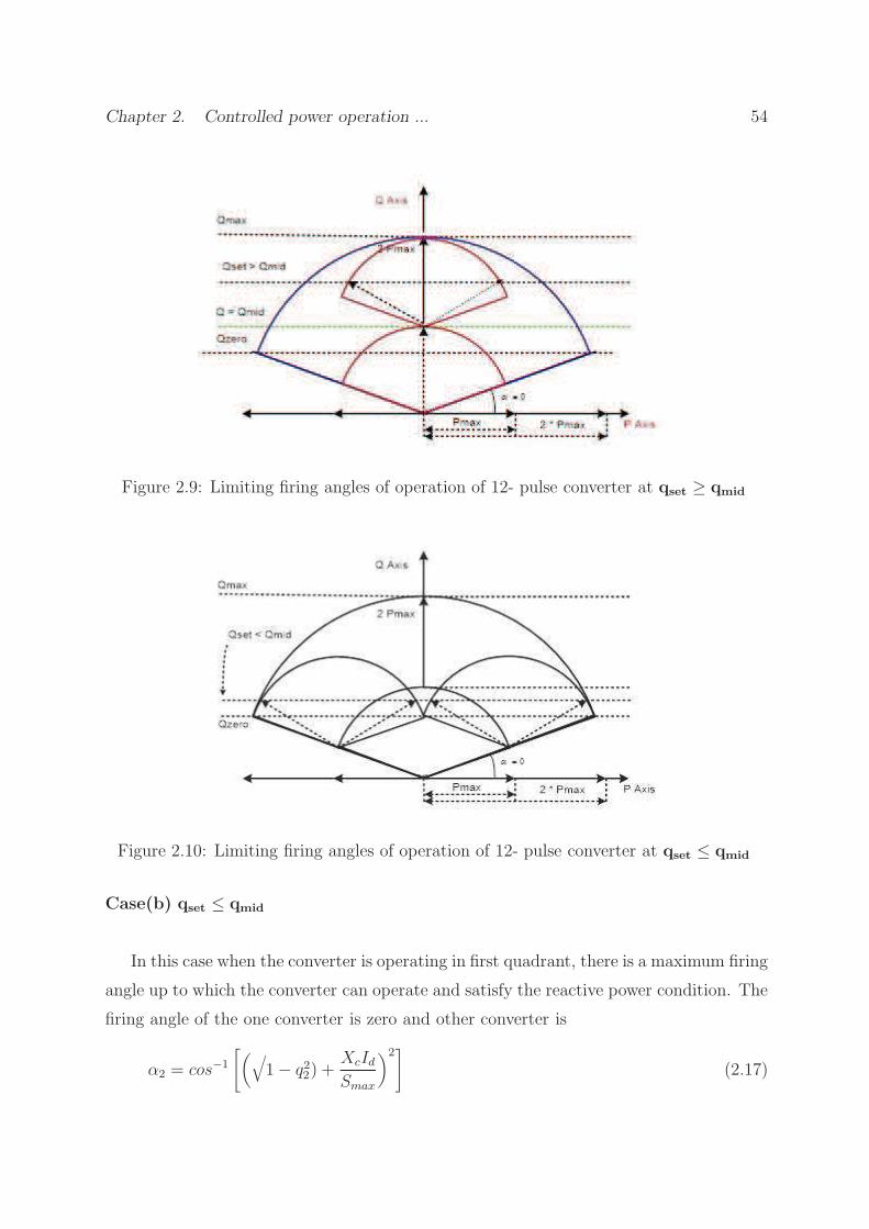
Figure 2.9: Limiting firing angles of operation of 12- pulse converter at qset ≥ qmid
Figure 2.10: Limiting firing angles of operation of 12- pulse converter at qset ≤ qmid
Case(b) qset ≤ qmid
In this case when the converter is operating in first quadrant, there is a maximum firing
angle up to which the converter can operate and satisfy the reactive power condition. The
firing angle of the one converter is zero and other converter is
α2 = cos−1[
(
√
1− q22) +XcId
Smax
)2]
(2.17)
Chapter 2. Controlled power operation ... 55
Or
α2 = π − cos−1[
(
√
1− q22) +XcId
Smax
)2]
(2.18)
This maximum firing angle for one converter occurs when the other converter operates
at a firing angle for minimum Q (i.e. α1). And when the 12-pulse converter is operating in
the second quadrant, and when one of the constituent converters is operating at minimum
Q when α1 = end stop, the minimum firing angle at which the converter must operate
satisfying the reactive power criteria is
α2 = cos−1[
(
√
1− q22) +XcId
Smax
)2]
(2.19)
Or
α2 = π − cos−1[
(
√
1− q22) +XcId
Smax
)2]
(2.20)
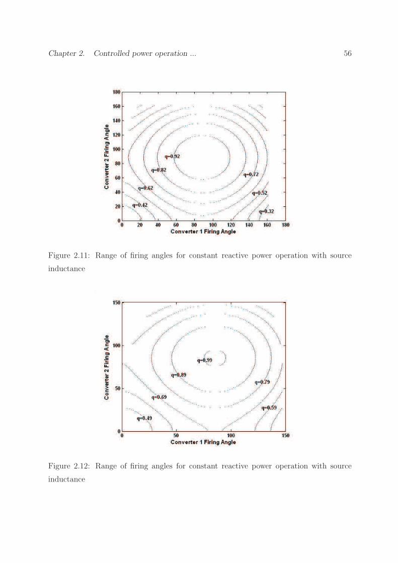
Figure 2.11 represents the range of firing angles at which the two converters need to
operate for different constant Var operating conditions. This figure depicts both the re-
gions of operation. As the value of the source inductance is varied, the region of operation
and range of is also varied. Figure 2.12 and Figure 2.13 shows the same effect for different
valus of source impedance. Same effect can also observed for variation of the load current
as shown in Figure 2.14 and Figure 2.15 with source impedance. Figure 2.11 represents
the range of firing angles at which the two converters need to operate for different constant
Var operating conditions. This figure depicts both the regions of operation. As the value
of the source inductance is varied, the region of operation and range of is also varied.
Figure 2.12 and Figure 2.13 shows the same effect for different valus of source impedance.
Same effect can also observed for variation of the load current as shown in Figure 2.14
and Figure 2.15 with source impedance.
Chapter 2. Controlled power operation ... 56
Figure 2.11: Range of firing angles for constant reactive power operation with source
inductance
Figure 2.12: Range of firing angles for constant reactive power operation with source
inductance
Chapter 2. Controlled power operation ... 57
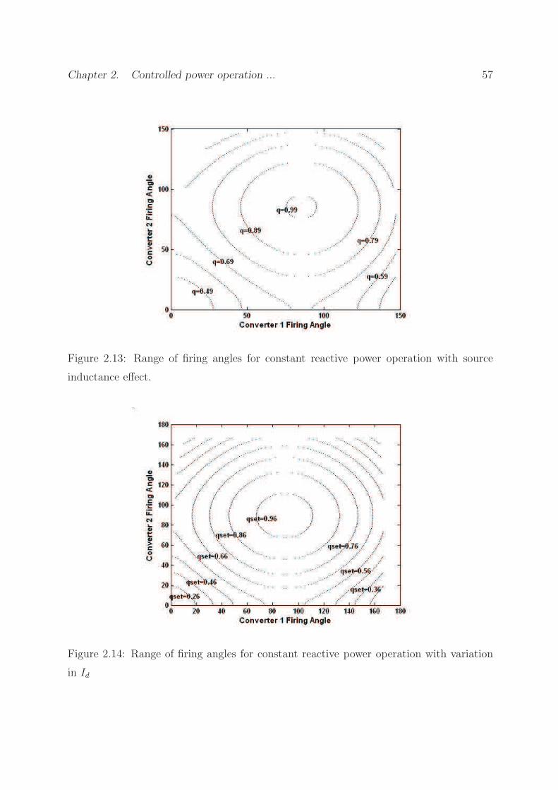
Figure 2.13: Range of firing angles for constant reactive power operation with source
inductance effect.
Figure 2.14: Range of firing angles for constant reactive power operation with variation
in Id
Chapter 2. Controlled power operation ... 58
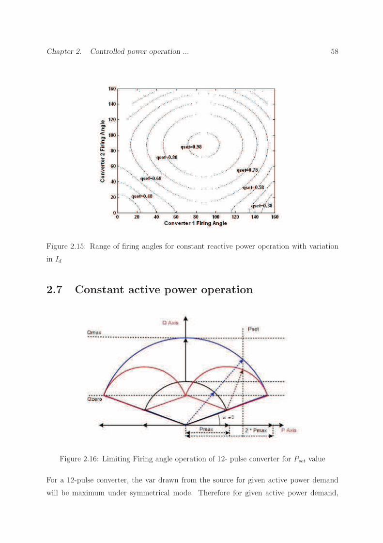
Figure 2.15: Range of firing angles for constant reactive power operation with variation
in Id
2.7 Constant active power operation
Figure 2.16: Limiting Firing angle operation of 12- pulse converter for Pset value
For a 12-pulse converter, the var drawn from the source for given active power demand
will be maximum under symmetrical mode. Therefore for given active power demand,
Chapter 2. Controlled power operation ... 59
only the minimum var condition has to be known. The 12-pulse converter operation in
constant active power mode can be explained using Figure 2.16. In this case, when the
converter is operated in asymmetrical mode, there will be a range of firing angles within
which both the converters must operated to generate constant active power.
Under certain operating condition the desired net active power Pset can be expressed in
per unit (p.u.) values as sum of the active power drawn by the each converter.
qset(p.u.) = (cosφ1 + cosφ2) ∗ 0.5 (2.21)
Or
qset(p.u.) =VdoId
Smax
(cosφ1 + cosφ2)−2XcI
2
d
Smax
(2.22)
at αi = 0
Pmax(p.u.) =(
1−XcId
Vdo
)
(2.23)
And
Pmin(p.u.) =(
cos(end− stop)−XcId
Vdo
)
(2.24)
So the Pset is varied between Pmin and Pmax From Figure 2.9 it is observed that, when
one of the converters is operated at α1 = 00, the other converter must operate at the
firing angle
α2 = cos−1[
2
(
Pset + I2dXc
Smax
)
− cosα1
]
(2.25)
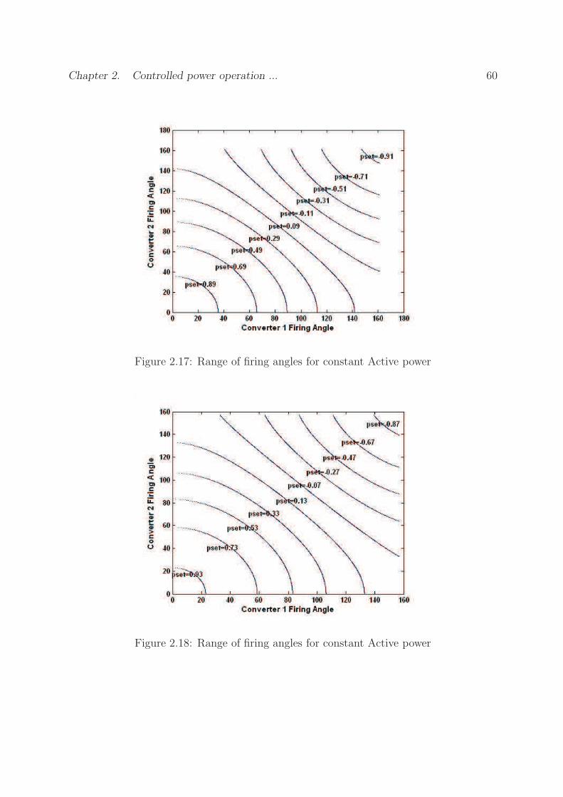
Figure 2.17 shows the curves for the various combinations of the firing angles at the
different values of Pset . At any value of active power transfer, the operating point of α1, α2
may lie at any point on the corresponding curve. The reactive power consumption depends
on the positioning of α1, α2 on that curve. It is observed that the freedom of choice of
α1, α2 reduces with the increase of active power transfer. As the source inductance is
increased this range of is also smaller and end stop limit for the both converter is also
decreasing. The value of the overlap angle is also depends on the load current. Figure
2.18 shows the variation the range of active power (p.u.) as the load current Id is varied.
Chapter 2. Controlled power operation ... 60
Figure 2.17: Range of firing angles for constant Active power
Figure 2.18: Range of firing angles for constant Active power
Chapter 2. Controlled power operation ... 61
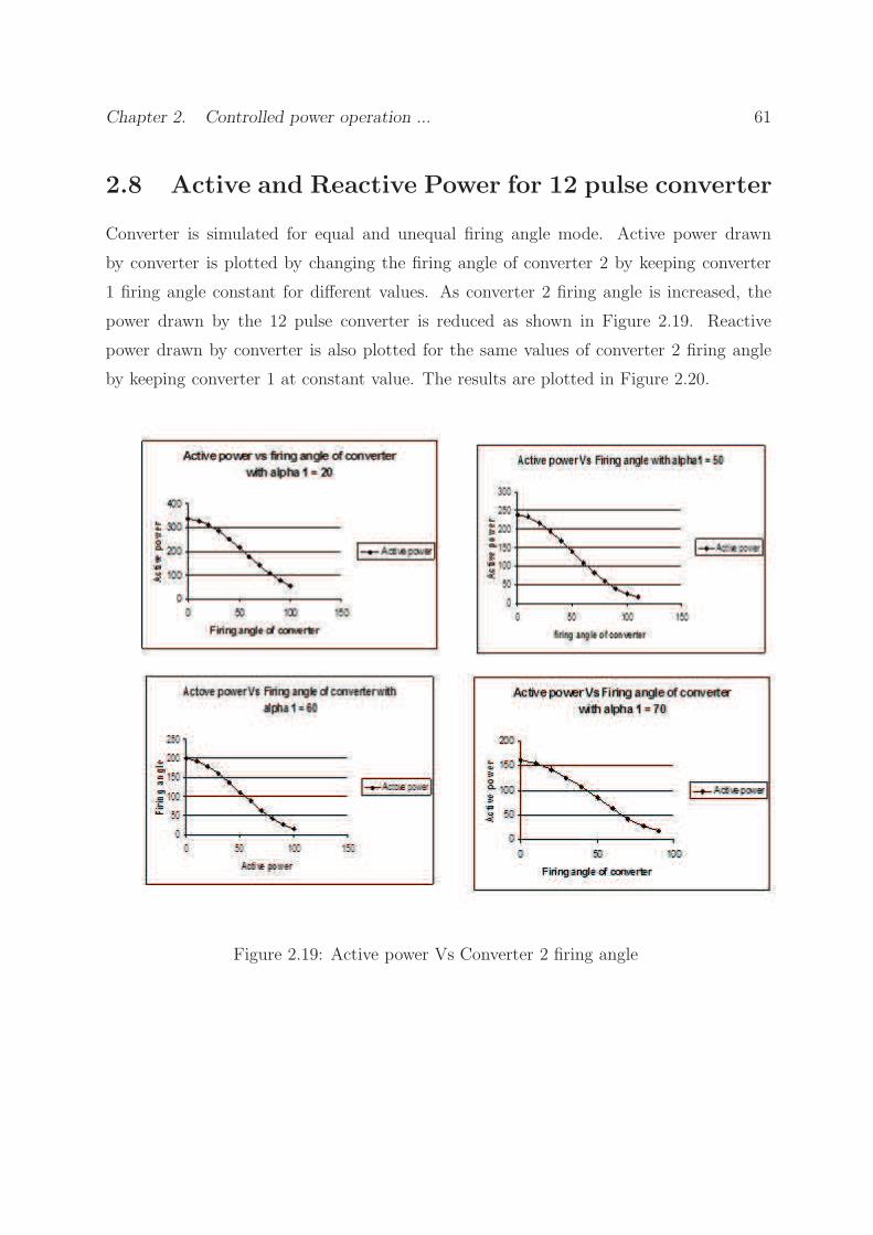
2.8 Active and Reactive Power for 12 pulse converter
Converter is simulated for equal and unequal firing angle mode. Active power drawn
by converter is plotted by changing the firing angle of converter 2 by keeping converter
1 firing angle constant for different values. As converter 2 firing angle is increased, the
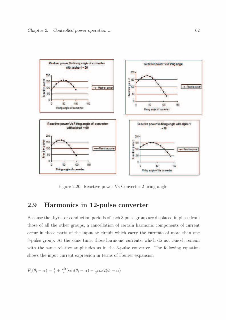
power drawn by the 12 pulse converter is reduced as shown in Figure 2.19. Reactive
power drawn by converter is also plotted for the same values of converter 2 firing angle
by keeping converter 1 at constant value. The results are plotted in Figure 2.20.
Figure 2.19: Active power Vs Converter 2 firing angle
Chapter 2. Controlled power operation ... 62
Figure 2.20: Reactive power Vs Converter 2 firing angle
2.9 Harmonics in 12-pulse converter
Because the thyristor conduction periods of each 3 pulse group are displaced in phase from
those of all the other groups, a cancellation of certain harmonic components of current
occur in those parts of the input ac circuit which carry the currents of more than one
3-pulse group. At the same time, those harmonic currents, which do not cancel, remain
with the same relative amplitudes as in the 3-pulse converter. The following equation
shows the input current expression in terms of Fourier expansion
F1(θi − α) = 1
3+√3
π[sin(θi − α)− 1
2cos2(θi − α)
Chapter 2. Controlled power operation ... 63
−1
4cos4(θi − α)− 1
5sin5(θi − α)− 1
7sin7(θi − α) + 1
8
cos8(θi − α) +1
10cos10(θi − α) +
1
11cos11(θi − α) +
1
13cos13(θi − α)........] (2.26)
2.9.1 Harmonic analysis of 6-pulse converter:
For a star connected primary of the input transformer, the supply current is given by
iSA = F1(θi − α)− F1(θi − α + π)
iSA = 2√3
π[sin(θi − α1)− 1
5sin5(θi − α1)− 1
7sin7(θi − α1)
+1
11sin11(θi − α1) +
1
13sin13(θi − α1)......] (2.27)
Thus the amplitude of the fundamental component of waveform is 3
π∗ peak value and
the harmonic components have the same frequencies and relative amplitudes as those of
star connected input.
iSB = 0.5F1(θi − α+ π
6)− 0.5F1(θi − α− 5π
6) + 0.5F1(θi − α− π
6)
−0.5F1(θi − α + 5π
6)
iSB = 3
π[sin(θi − α2) +
1
5sin5(θi − α2) +
1
7sin7(θi − α2) +
1
11sin11(θi − α2)
+ 1
13sin13(θi − α2).............]
2.9.2 Harmonic analysis of 12-pulse converter:
For obtaining a constant Var operation with wide-range of active power control, the 12-
pulse converter has to be operated under asymmetrical mode. Under this mode (6n± 1)
input current harmonics for all integral values of n appear in the supply. Where as, in
symmetrical mode, only (6n± 1) current harmonics for all n= even integers are present.
The general Fourier series expressions of (6n ± 1) harmonic components of the primary
Chapter 2. Controlled power operation ... 64
input current in a 12-pulse converter can be expressed as follows:
For all odd value of n,
I6n±1 =sin((6n± 1)(α1−α2
2))cos((6n± 1)(wt− (α1−α2
2)))
(6n± 1) ∗ cos(α1−α2
2)sin(wt− (α1−α2
2))
(2.28)
And, for all even value of n,
I6n±1 =cos((6n± 1)(α1−α2
2))cos((6n± 1)(wt− (α1−α2
2)))
(6n± 1) ∗ cos(α1−α2
2)sin(wt− (α1−α2
2))
(2.29)
where,
α1= Firing angle of converter 1
α2= Firing angle of converter 2
The above expressions are ratio of harmonic magnitudes to the fundamental at those
values of converter firing angles α1 and α2.
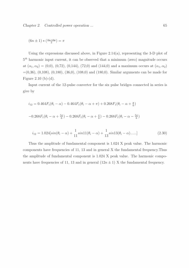
Figure 2.21 presents the 3D plot of per unit 6n ± 1 harmonic magnitudes for n=1,2
of source current for simultaneous variation in firing angles of both the converters. It
can also be observed from the figure that the maximum and minimum values of the p.u
harmonics occur alternately at different combinations of α1 and α2 which can be obtained
by the relationship expressed as follows:
For n=odd, the magnitude of the corresponding harmonic is zero when,
(6n± 1) ∗ (α1−α2
2) = π
And is maximum when,
(6n± 1) ∗ (α1−α2
2) = π
2
For n=even, the magnitude of the corresponding harmonic is zero when,
(6n± 1) ∗ (α1−α2
2) = π
2
And is maximum when,
Chapter 2. Controlled power operation ... 65
(6n± 1) ∗ (α1−α2
2) = π
Using the expressions discussed above, in Figure 2.14(a), representing the 3-D plot of
5th harmonic input current, it can be observed that a minimum (zero) magnitude occurs
at (α1, α2) = (0,0), (0,72), (0,144), (72,0) and (144,0) and a maximum occurs at (α1, α2)
=(0,36), (0,108), (0,180), (36,0), (108,0) and (180,0). Similar arguments can be made for
Figure 2.10 (b)-(d).
Input current of the 12-pulse converter for the six pulse bridges connected in series is
give by
i12 = 0.464F1(θi − α)− 0.464F1(θi − α + π) + 0.268F1(θi − α + π
6)
−0.268F1(θi − α + 5π
6)− 0.268F1(θi − α + π
6)− 0.268F1(θi − α− 5π
6)
i12 = 1.024[sin(θi − α) +1
11sin11(θi − α) +
1
13sin13(θi − α)......] (2.30)
Thus the amplitude of fundamental component is 1.024 X peak value. The harmonic
components have frequencies of 11, 13 and in general X the fundamental frequency.Thus
the amplitude of fundamental component is 1.024 X peak value. The harmonic compo-
nents have frequencies of 11, 13 and in general (12n± 1) X the fundamental frequency.
Chapter 2. Controlled power operation ... 66
Figure 2.21: per unit 5th, 7th, 11th and 13th harmonics for simultaneous variation of
converter 1 and 2 firing angles
Chapter 2. Controlled power operation ... 67
2.10 Harmonic analysis of the 12-pulse converter op-
erating under unequal firing angle
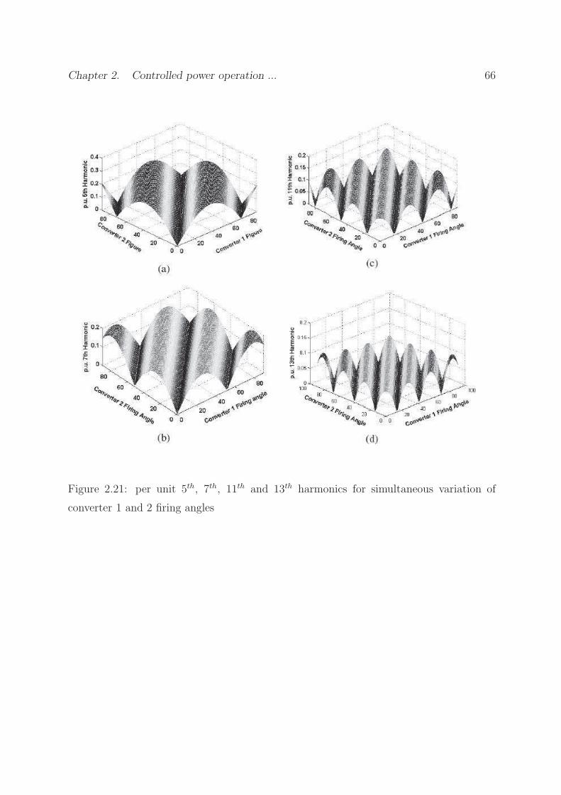
Figure 2.22: % THD 5th, 7th, 11th and 13th harmonic component Vs Converter 2 firing
angle
12 pulse converter is simulated for equal and unequal mode of operation. The % Total
Harmonic Distortion (THD) is measured along with 5th, 7th, 11th and 13th order harmonic
current component for different values of converter 2 firing angle while keeping converter
1 firing angle constant for different values. As shown in Figure 2.22, it follows (6n ± 1)
Chapter 2. Controlled power operation ... 68
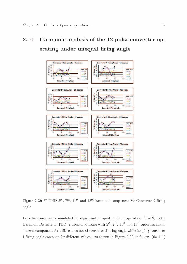
for equal firing angle and (12n ± 1) for unequal firing angle mode. The total patterns
are added for % THD and plotted as shown in Figure 2.23 where variation of % THD
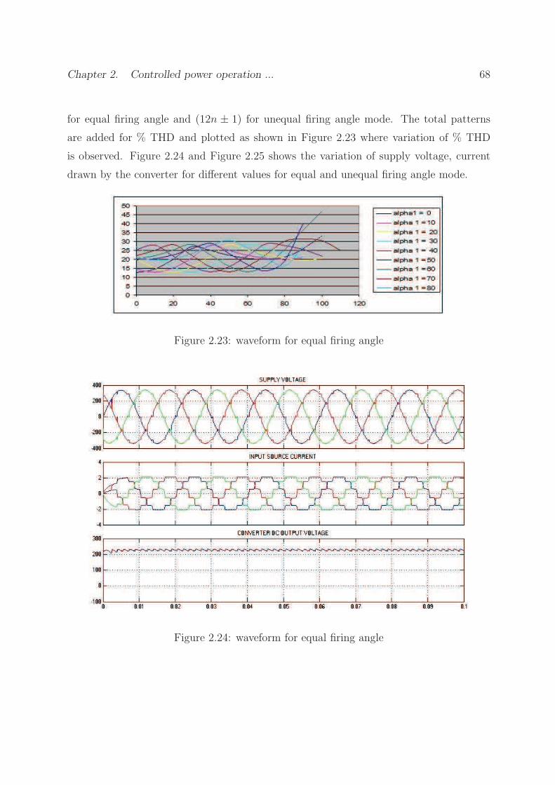
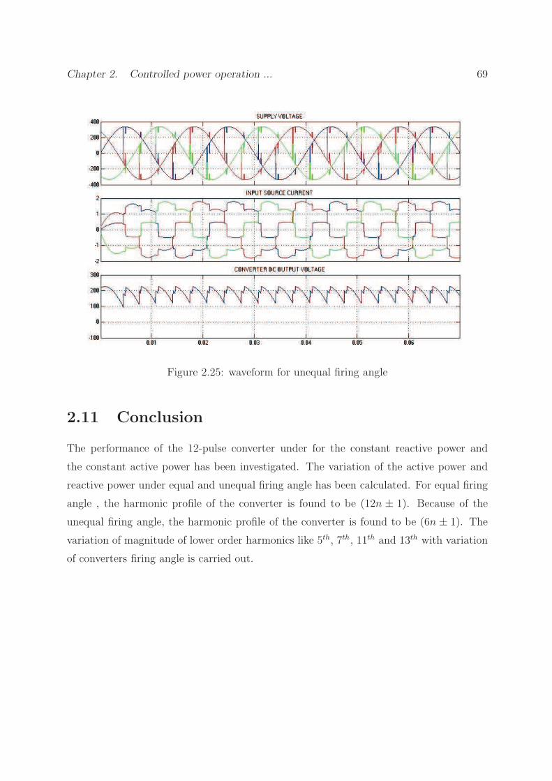
is observed. Figure 2.24 and Figure 2.25 shows the variation of supply voltage, current
drawn by the converter for different values for equal and unequal firing angle mode.
Figure 2.23: waveform for equal firing angle
Figure 2.24: waveform for equal firing angle
Chapter 2. Controlled power operation ... 69
Figure 2.25: waveform for unequal firing angle
2.11 Conclusion
The performance of the 12-pulse converter under for the constant reactive power and
the constant active power has been investigated. The variation of the active power and
reactive power under equal and unequal firing angle has been calculated. For equal firing
angle , the harmonic profile of the converter is found to be (12n ± 1). Because of the
unequal firing angle, the harmonic profile of the converter is found to be (6n ± 1). The
variation of magnitude of lower order harmonics like 5th, 7th, 11th and 13th with variation
of converters firing angle is carried out.