Equity Valuation Models

Chapter 18

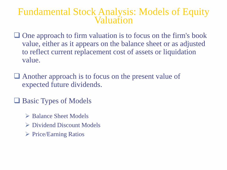
One approach to firm valuation is to focus on the firm's book value, either as it appears on the balance sheet or as adjusted to reflect current replacement cost of assets or liquidation value.

Another approach is to focus on the present value of expected future dividends.

Basic Types of Models

Balance Sheet Models

Dividend Discount Models

Price/Earning Ratios

Fundamental Stock Analysis: Models of Equity Valuation

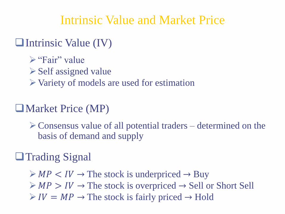
Intrinsic Value (IV)

“Fair” value

Self assigned value

Variety of models are used for estimation

Market Price (MP)

Consensus value of all potential traders – determined on the basis of demand and supply

Trading Signal

𝑀𝑃 < 𝐼𝑉 → The stock is underpriced → Buy

𝑀𝑃 > 𝐼𝑉 → The stock is overpriced → Sell or Short Sell

𝐼𝑉 = 𝑀𝑃 → The stock is fairly priced → Hold

Intrinsic Value and Market Price

VD

ko

t

tt

( )11

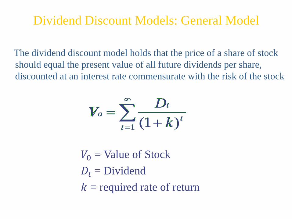
𝑉0 = Value of Stock

𝐷𝑡 = Dividend

𝑘 = required rate of return

Dividend Discount Models: General Model

The dividend discount model holds that the price of a share of stock

should equal the present value of all future dividends per share,

discounted at an interest rate commensurate with the risk of the stock

VD

ko

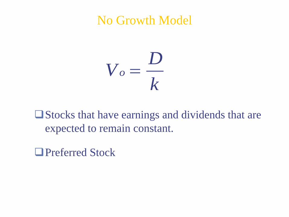
Stocks that have earnings and dividends that are

expected to remain constant.

Preferred Stock

No Growth Model

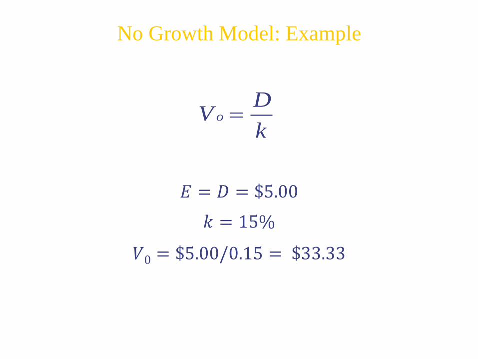
𝐸 = 𝐷 = $5.00

𝑘 = 15%

𝑉0 = $5.00/0.15 = $33.33

VD

ko

No Growth Model: Example

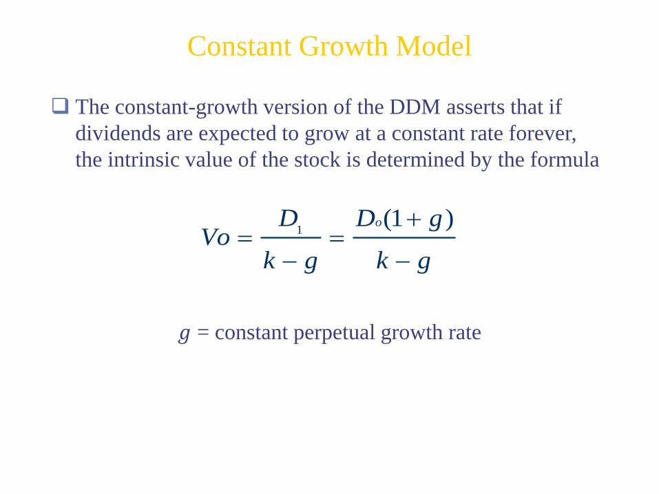
Constant Growth Model

The constant-growth version of the DDM asserts that if

dividends are expected to grow at a constant rate forever,

the intrinsic value of the stock is determined by the formula

𝑔 = constant perpetual growth rate

1(1 )oD D g

Vok g k g

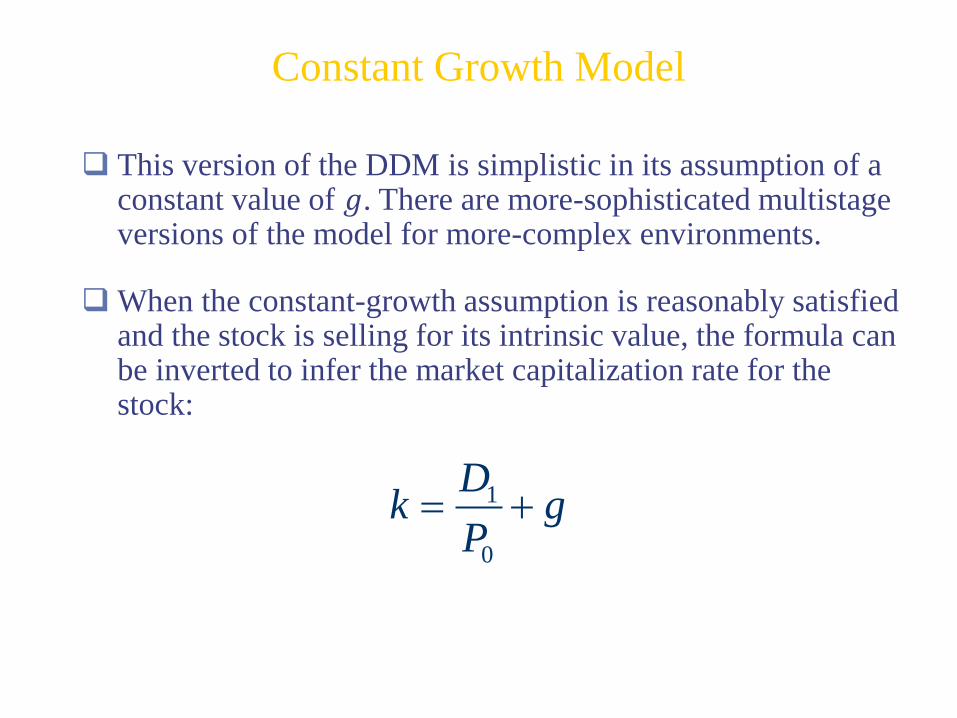
Constant Growth Model

This version of the DDM is simplistic in its assumption of a constant value of 𝑔. There are more-sophisticated multistage versions of the model for more-complex environments.

When the constant-growth assumption is reasonably satisfied and the stock is selling for its intrinsic value, the formula can be inverted to infer the market capitalization rate for the stock:

1

0

Dk g

P

Constant Growth Model

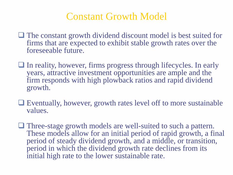
The constant growth dividend discount model is best suited for firms that are expected to exhibit stable growth rates over the foreseeable future.

In reality, however, firms progress through lifecycles. In early years, attractive investment opportunities are ample and the firm responds with high plowback ratios and rapid dividend growth.

Eventually, however, growth rates level off to more sustainable values.

Three-stage growth models are well-suited to such a pattern. These models allow for an initial period of rapid growth, a final period of steady dividend growth, and a middle, or transition, period in which the dividend growth rate declines from its initial high rate to the lower sustainable rate.

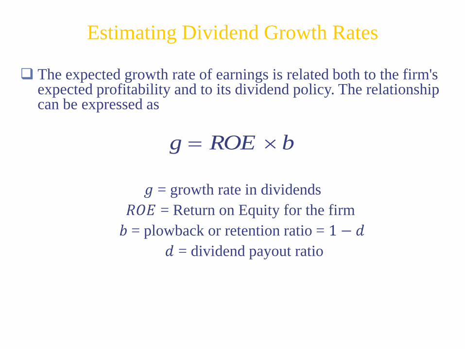
g ROE b

The expected growth rate of earnings is related both to the firm's expected profitability and to its dividend policy. The relationship can be expressed as

𝑔 = growth rate in dividends

𝑅𝑂𝐸 = Return on Equity for the firm

𝑏 = plowback or retention ratio = 1 − 𝑑

𝑑 = dividend payout ratio

Estimating Dividend Growth Rates

1DVo

k g

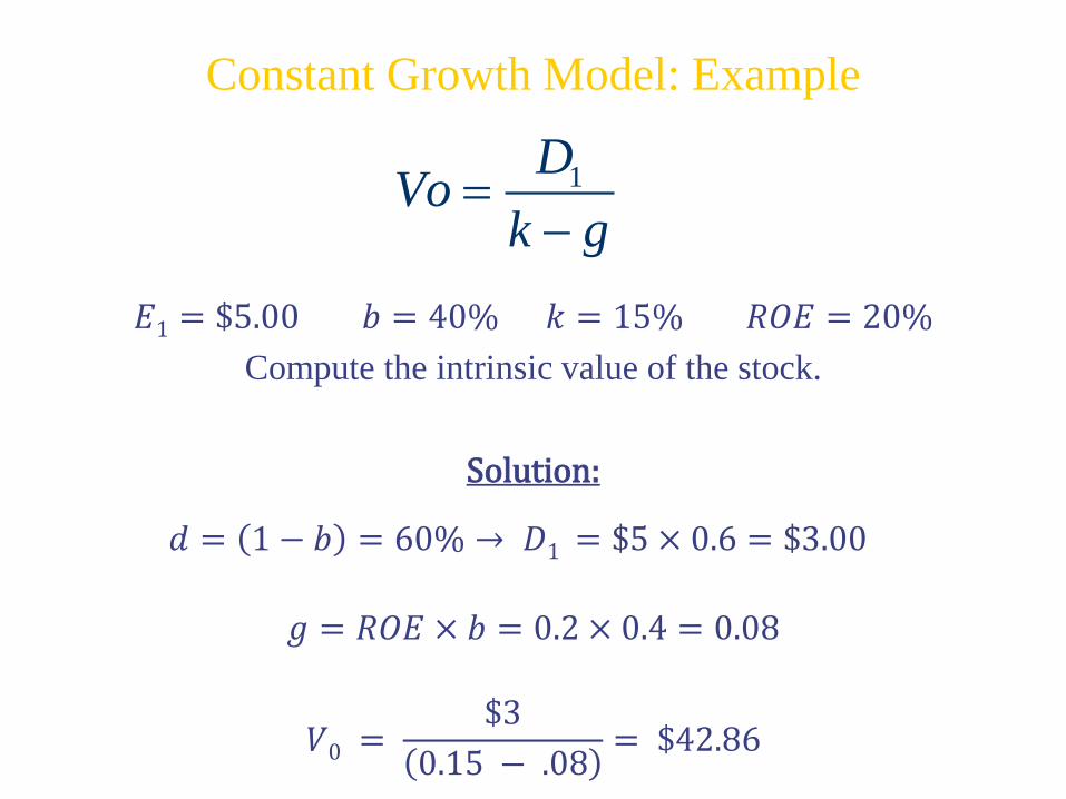
𝐸1 = $5.00 𝑏 = 40% 𝑘 = 15% 𝑅𝑂𝐸 = 20%

Compute the intrinsic value of the stock.

Solution:

𝑑 = 1 − 𝑏 = 60% → 𝐷1 = $5 × 0.6 = $3.00

𝑔 = 𝑅𝑂𝐸 × 𝑏 = 0.2 × 0.4 = 0.08

𝑉0 =$3

0.15 − .08= $42.86

Constant Growth Model: Example

1 2

20...

(1 ) (1 ) (1 )N N

N

D PD DV

k k k

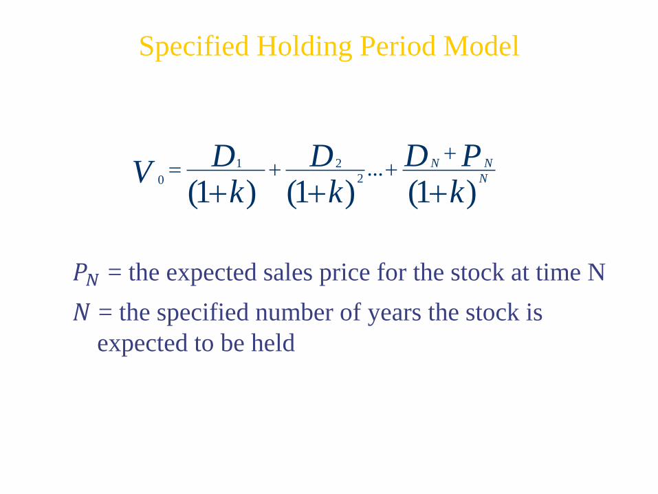
𝑃𝑁 = the expected sales price for the stock at time N

𝑁 = the specified number of years the stock is

expected to be held

Specified Holding Period Model

1

1 1 1(1 )

( )

o

o

EV PVGO

k

E D ED gPVGO

k g k k g k

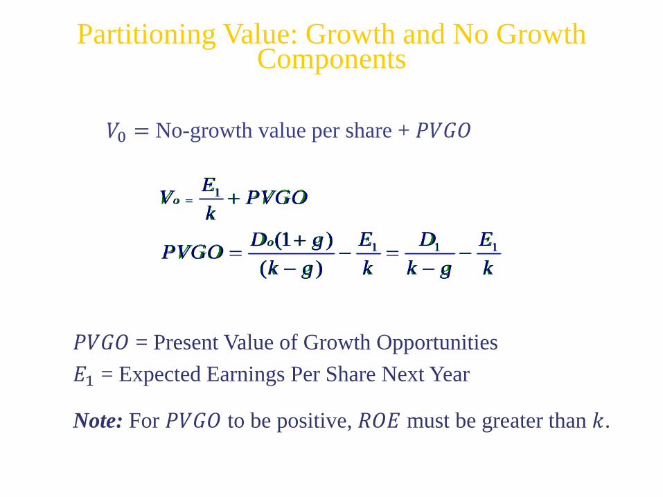
𝑃𝑉𝐺𝑂 = Present Value of Growth Opportunities

𝐸1 = Expected Earnings Per Share Next Year

Note: For 𝑃𝑉𝐺𝑂 to be positive, 𝑅𝑂𝐸 must be greater than 𝑘.

Partitioning Value: Growth and No Growth Components

𝑉0 = No-growth value per share + 𝑃𝑉𝐺𝑂

For 𝑃𝑉𝐺𝑂 to be positive, 𝑅𝑂𝐸 must be greater than 𝑘

If 𝑃𝑉𝐺𝑂 =𝐷1

𝑘−𝑅𝑂𝐸×𝑏−

𝐸1

𝑘> 0

→𝐷1

𝑘 − 𝑅𝑂𝐸 × 𝑏>𝐸1𝑘

→ 𝐷1 > 𝐸1 −𝐸1𝑘𝑅𝑂𝐸 × 𝑏

→𝐸1𝑘𝑅𝑂𝐸 × 𝑏 > 𝐸1 − 𝐷1

→ 𝑅𝑂𝐸 >(𝐸1−𝑑𝐸1)𝑘

𝑏𝐸1=𝐸1 1 − 𝑑 𝑘

𝑏𝐸1=𝑏𝐸1𝑏𝐸1

𝑘 = 𝑘

→ 𝑅𝑂𝐸 > 𝑘

𝑅𝑂𝐸 = 20% 𝑑 = 60% 𝑏 = 40%

𝐸1 = $5.00 𝐷1 = $3.00 𝑘 = 15%

𝑔 = 0.20 × 0.40 = .08 𝑜𝑟 8%

Partitioning Value: Example

$3$42.86

(0.15 0.08)

$5$33.33

0.15

$42.86 $33.33 $9.52

o

o

V

NGV

PVGO

𝑉0 = value with growth

𝑁𝐺𝑉0 = no growth component value

𝑃𝑉𝐺𝑂 = Present Value of Growth Opportunities

In this example, 𝑅𝑂𝐸 > 𝑘

If 𝑅𝑂𝐸 = 15%, 𝑃𝑉𝐺𝑂 = 0. If 𝑅𝑂𝐸 =10%, 𝑃𝑉𝐺𝑂 = −15.59

Partitioning Value: Example

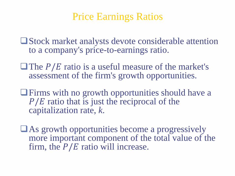
Stock market analysts devote considerable attention to a company's price-to-earnings ratio.

The 𝑃/𝐸 ratio is a useful measure of the market's assessment of the firm's growth opportunities.

Firms with no growth opportunities should have a 𝑃/𝐸 ratio that is just the reciprocal of the capitalization rate, k.

As growth opportunities become a progressively more important component of the total value of the firm, the 𝑃/𝐸 ratio will increase.

Price Earnings Ratios

Price Earnings Ratios

𝑃/𝐸 Ratios are a function of two factors

Required Rates of Return (𝑘)

Expected growth in Dividends

Uses

Relative valuation

Extensive Use in industry

10

0

1

1

EP

k

P

E k

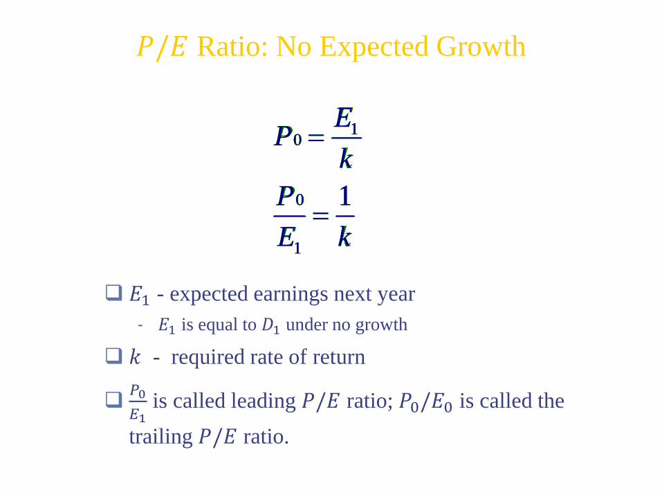
𝐸1 - expected earnings next year

- 𝐸1 is equal to 𝐷1 under no growth

𝑘 - required rate of return

𝑃0

𝐸1is called leading 𝑃/𝐸 ratio; 𝑃0/𝐸0 is called the

trailing 𝑃/𝐸 ratio.

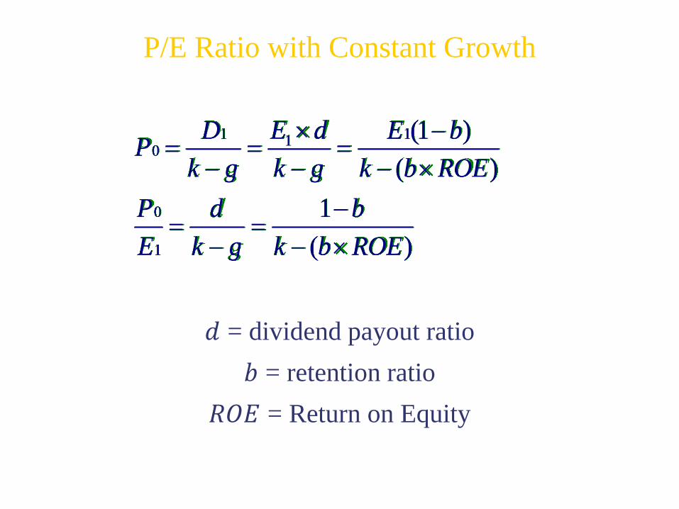
𝑃/𝐸 Ratio: No Expected Growth

1 110

0

1

(1 )

( )

1

( )

E dD E bP

k g k g k b ROE

P d b

E k g k b ROE

𝑑 = dividend payout ratio

𝑏 = retention ratio

𝑅𝑂𝐸 = Return on Equity

P/E Ratio with Constant Growth

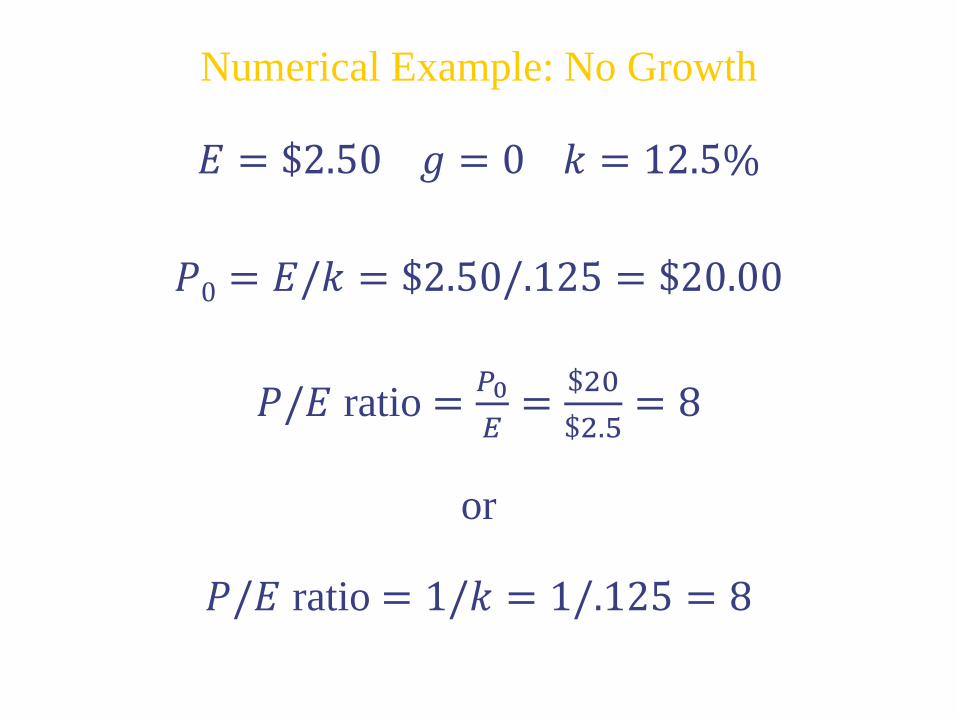
𝐸 = $2.50 𝑔 = 0 𝑘 = 12.5%

𝑃0 = 𝐸/𝑘 = $2.50/.125 = $20.00

𝑃/𝐸 ratio =𝑃0

𝐸=

$20

$2.5= 8

or

𝑃/𝐸 ratio = 1/𝑘 = 1/.125 = 8

Numerical Example: No Growth

𝑏 = 60% 𝑅𝑂𝐸 = 15% 𝑑 = (1 − 𝑏) = 40%

𝐸1 = $2.50 1 + 0.15 0.6 = $2.73

𝐷1 = $2.73(0.4) = $1.09

𝑘 = 12.5% 𝑔 = 9%

𝑃0 =$1.09

0.125 − .09= $31.14

Leading 𝑃/𝐸 =$31.14

$2.73= 11.4

or

Leading 𝑃/𝐸 =𝑑

𝑘−𝑔=

0.4

0.125−0.09= 11.4

Numerical Example with Growth

Pitfalls in P/E Analysis

Many analysts form their estimate of a stock's value by

multiplying their forecast of next year's 𝐸𝑃𝑆 by a 𝑃/𝐸 multiple

derived from some empirical rule.

This rule can be consistent with some version of the 𝐷𝐷𝑀,

although often it is not.

Often people use average 𝑃/𝐸 ratio using past data, which

ignores the growth opportunity of the firm.

Use of accounting earnings also has its problems, e.g.,

- Historical costs in depreciation and inventory valuation: during high

inflation period, the use of historical cost would underestimate cost thus

overestimate earnings and underestimate 𝑃/𝐸 ratio.

Inflation and Equity Valuation

Inflation has an impact on real stock returns.

Research shows that real rates of return are lower with

higher rates of inflation.

Remember Fisher effect?

𝑟 = 𝑅– 𝑖 (approximate)

Empirical research shows that inflation has an

adverse effect on equity values.

Inflation and Equity Valuation

One reason is the lower real after-tax earnings and dividends attributable to inflation-induced distortions in the tax system.

Often govt. tries to implement contractionary fiscal policy i.e. raise taxes to reduce inflationary pressure.

Practice Problems

Chapter 18:

4, 5, 6, 7, 8, 9, 10, 11