Bioinformatics – From Genomes to Therapies (volume I, pp. 491-539) IN PRESS

To be published in 12/2006.

Editor: Thomas Lengauer

Publisher: Wiley-VCH

Chapter 15: RNA tertiary structure prediction François Major and Philippe Thibault

Institute for Research in Immunology and Cancer and Department of Computer Science and

Operations Research, Université de Montréal, PO Box 6128, downtown station, Montreal,

Quebec, Canada H3C 3J7.

1 GOAL AND CHAPTER ORGANIZATION

During the last decade, the number of high-quality X-ray crystallographic ribonucleic acid (RNA)

three-dimensional (3-D) structures has increased significantly, and the resolution of the large

ribosomal subunit crystal structure was considered a major step towards a better understanding of

RNA tertiary structure and folding. The recent discovery of the RNA interference (RNAi)

pathway (see Chapter 46) has also contributed greatly to the popularity of RNAs, by suggesting

their direct implication in genetic expression and regulation. More than ever, determining rapidly

and precisely the tertiary structure and function of non-coding RNAs is a crucial step towards our

understanding of several cellular metabolic pathways.

This chapter is dedicated to the RNA tertiary structure prediction problem, the determination of

the complete set of chemical interactions, and therefore 3-D fold, of an RNA from sequence data.

To achieve RNA structure prediction, one needs to discover and apply its structural and

architectural principles, which can be learnt from thermodynamics, as well as from structural data

gathered from X-ray crystallography and other high-resolution, but also low-resolution,

experimental methods. Here, we present a series of nomenclatures and formalisms to describe

RNA tertiary structure, as well as computer data structures and algorithms that implement three

important research activities with the aim of solving RNA tertiary structure prediction:

annotation, motif discovery, and modeling.

We present in Section 2 a series of RNA structure components and the terms employed by the

RNA specialists to discuss them, their universe of discourse, that are nowadays referred to as their

ontology. First, we present an ontology of nucleotide conformations and binary interactions.

Then, visual or automated inspection of RNA 3-D structures is necessary to depict higher-order

architectural principles (the next abstraction levels). In Section 3, we introduce a definition of

n-ary nucleotide interactions to describe RNA higher-order motifs, which are found repeated in

2

RNA structures and are often linked to specific structural and biochemical functions, and an

approach to search them. Finally, in Section 4, we present how accurate computer models of

RNA tertiary structures can be generated, and how, by challenging them experimentally, they

bring insights about function.

The flowchart in Figure 1 shows the relationships between structural data and hypotheses, and

how the research activities that aim at solving the RNA tertiary structure prediction problem are

intimately linked. The high-resolution (better than 3 Å) X-ray crystal structures of the Protein

Data Bank (PDB) (www.rcsb.org) [1] constitute an excellent structural (learning) data set that

aliments the research, and from which RNA tertiary structure prediction algorithms can be

inspired and tested. The characterization and formalization of RNA structural data (annotation),

the discovery of high-order components (motif discovery), and the building of RNA tertiary

structure models (modeling) contribute directly to the learning and discovery processes, leading

to new knowledge that is fed back to research.

An ultimate solution to the tertiary structure prediction problem will provide us invaluable

structural information, and will allow us to determine the function and the evolutionary

relationships of RNAs. Knowledge of RNA tertiary structure impacts in molecular medicine

techniques to control genetic expression, and to inhibit and activate specific cellular functions.

The cell controls its own genetic expression by processing micro RNAs through the RNAi

pathway. As we discover and characterize the elements of RNAi, we learn how to design RNAs

that interfere and block the expression of several genes. Knowledge of the structure and of the

interplay between the RNAs and the other RNAi elements is fundamental. Alternatively, we

could target the natural micro RNAs of the cell using drugs. Again, knowledge of the targeted

RNA structure is necessary to design accurate drugs. Targeting the non-coding RNAs of the cell

allows us to manipulate its fundamental mechanisms prior to protein translation; like playing with

the “source code” of the cell. Antibiotics such as aminoglycosides and macrolides target the site-

A of prokaryotic ribosomes, which block protein translation and kill them. The search and

discovery of other sites in the ribosome or in other RNAs involved in such fundamental

mechanisms require the determination of their tertiary structure if we want to design drugs

capable of inhibiting them. Ribozymes are catalytic RNAs that can cleave a substrate efficiently

and precisely. For instance, ribozymes can be used to cleave a messenger prior to its translation

by the ribosome. Here again, knowledge of the tertiary structure of ribozymes and of their

complex with the substrate is essential for rational design.

3

2 ANNOTATION

The annotation of an RNA tertiary structure is the assignment (manual or automated) of

appropriate symbols, taken from the RNA ontology, that apply to a given RNA. One can see

annotation as a data refinement process that complements the 3-D atomic coordinates, a different

and perhaps higher level of abstraction which can be thought of as an efficient and sound data

format to study further tertiary structures.

A human RNA expert recognizes the attributes of tertiary structures by visualization using

interactive computer graphics, and can therefore annotate a given RNA 3-D structure. An

automated procedure loads the RNA 3-D atomic coordinates in memory and then computes the

annotations. Gendron, Lemieux, and Major have developed a computer program, MC-Annotate,

which annotates a fraction of the current RNA ontology, in particular the terms related to the

nucleotide conformations, as well as base stacking (bs) and base pairing (bp) types [2] (see

Sections 2.2). MC-Annotate can be run over the Web (www-lbit.iro.umontreal.ca; under Research

and MC-Annotate). Westhof and co-workers, in collaboration with the PDB, developed RNAView,

a computer program that draws the secondary structure of an RNA while using the LW

nomenclature (see Sections 2.2.2) to display the bp types [3]. RNAView is accessible on the Web

(ndbserver.rutgers.edu/services).

In this Section, we present a series of RNA tertiary structure attributes, and how they can be

computed from 3-D atomic coordinates, from X-ray crystallographic structures of the PDB. We

present the nucleotide conformations (Section 2.1) and interactions (Section 2.2), which are

needed to define higher-order RNA components (Section 3) and to build and describe RNA

tertiary structure (Section 4).

2.1 Nucleotide conformations

RNAs are polymeric molecules. The monomer unit is a ribonucleotide, or simply nucleotide,

which divides in three units: the nucleobase (or simply base), the ribose, and the phosphate group

(see Figure 2). There are four bases: adenine (A), guanine (G), cytosine (C), and uracil (U). The

four bases partition in two families: the pyrimidines (Y) C and U, which are composed of a single

pyrimidine ring, and the purines (R) A and G, which are composed of the fusion of the pyrimidine

ring (C4H4N2) and of an imidazole ring (C3H4N2). The International Union of Pure and Applied

Chemistry (IUPAC) defined a one-letter code for all possible subsets of {A, C, G, U} (shown in

Table 1).

The ribose links the phosphate groups to which the bases are attached by the glycosidic bond:

C1’-N9 in purines and C1’-N1 in pyrimidines. The riboses and the phosphate groups constitute

4

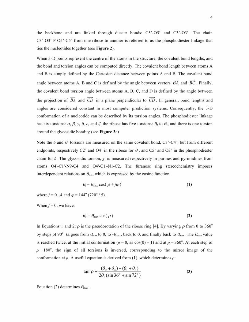
the backbone and are linked through diester bonds: C5’-O5’ and C3’-O3’. The chain

C3’-O3’-P-O5’-C5’ from one ribose to another is referred to as the phosphodiester linkage that

ties the nucleotides together (see Figure 2).

When 3-D points represent the centre of the atoms in the structure, the covalent bond lengths, and

the bond and torsion angles can be computed directly. The covalent bond length between atoms A

and B is simply defined by the Cartesian distance between points A and B. The covalent bond

angle between atoms A, B and C is defined by the angle between vectors

!

BA and BC . Finally,

the covalent bond torsion angle between atoms A, B, C, and D is defined by the angle between

the projection of BA and CD in a plane perpendicular to CD . In general, bond lengths and

angles are considered constant in most computer prediction systems. Consequently, the 3-D

conformation of a nucleotide can be described by its torsion angles. The phosphodiester linkage

has six torsions: α, β, γ, δ, ε, and ζ, the ribose has five torsions: θ0 to θ4, and there is one torsion

around the glycosidic bond: χ (see Figure 3a).

Note the δ and θ1 torsions are measured on the same covalent bond, C3’-C4’, but from different

endpoints, respectively C2’ and O4’ in the ribose for θ1, and C5’ and O3’ in the phosphodiester

chain for δ. The glycosidic torsion, χ, is measured respectively in purines and pyrimidines from

atoms O4'-C1'-N9-C4 and O4'-C1'-N1-C2. The furanose ring stereochemistry imposes

interdependent relations on θ0-4, which is expressed by the cosine function:

θj = θmax cos( ρ + jϕ ) (1)

where j = 0...4 and ϕ = 144o (720o / 5).

When j = 0, we have:

θ0 = θmax cos( ρ ) (2)

In Equations 1 and 2, ρ is the pseudorotation of the ribose ring [4]. By varying ρ from 0 to 360o

by steps of 90o, θ0 goes from θmax to 0, to -θmax, back to 0, and finally back to θmax. The θmax value

is reached twice, at the initial conformation (ρ = 0, as cos(0) = 1) and at ρ = 360o. At each step of

ρ + 180o, the sign of all torsions is inversed, corresponding to the mirror image of the

conformation at ρ. A useful equation is derived from (1), which determines ρ:

)72sin36(sin2

)()( tan

0

3142

oo+

+!+=

"

""""# (3)

Equation (2) determines θmax.

5

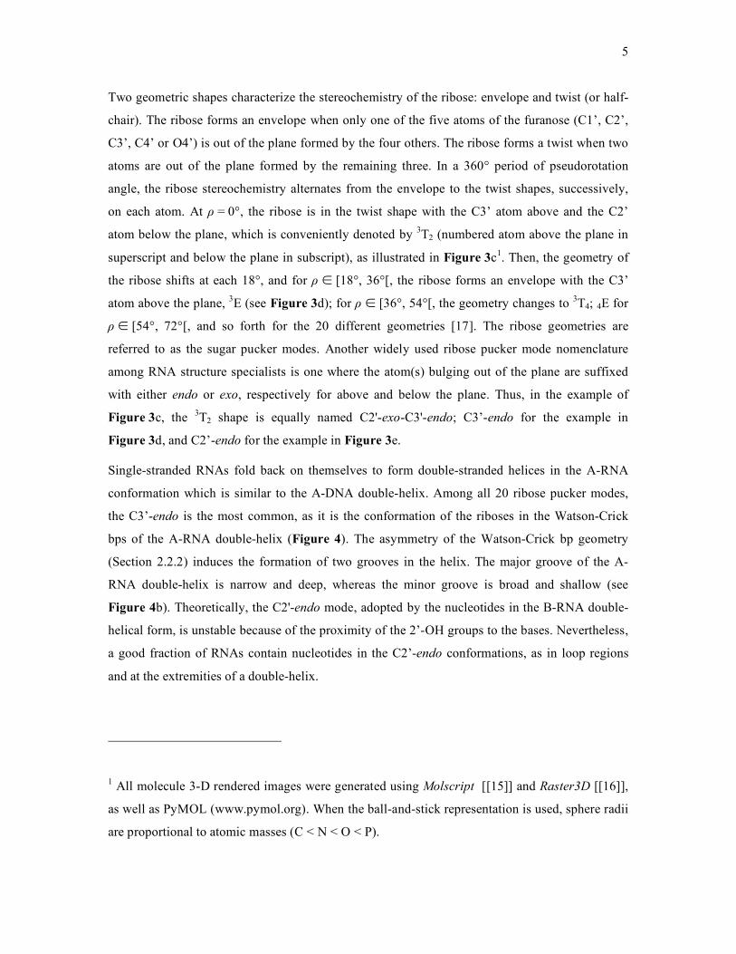
Two geometric shapes characterize the stereochemistry of the ribose: envelope and twist (or half-

chair). The ribose forms an envelope when only one of the five atoms of the furanose (C1’, C2’,

C3’, C4’ or O4’) is out of the plane formed by the four others. The ribose forms a twist when two

atoms are out of the plane formed by the remaining three. In a 360° period of pseudorotation

angle, the ribose stereochemistry alternates from the envelope to the twist shapes, successively,

on each atom. At ρ = 0°, the ribose is in the twist shape with the C3’ atom above and the C2’

atom below the plane, which is conveniently denoted by 3T2 (numbered atom above the plane in

superscript and below the plane in subscript), as illustrated in Figure 3c1. Then, the geometry of

the ribose shifts at each 18°, and for ρ ! [18°, 36°[, the ribose forms an envelope with the C3’

atom above the plane, 3E (see Figure 3d); for ρ ! [36°, 54°[, the geometry changes to 3T4; 4E for

ρ ! [54°, 72°[, and so forth for the 20 different geometries [17]. The ribose geometries are

referred to as the sugar pucker modes. Another widely used ribose pucker mode nomenclature

among RNA structure specialists is one where the atom(s) bulging out of the plane are suffixed

with either endo or exo, respectively for above and below the plane. Thus, in the example of

Figure 3c, the 3T2 shape is equally named C2'-exo-C3'-endo; C3’-endo for the example in

Figure 3d, and C2’-endo for the example in Figure 3e.

Single-stranded RNAs fold back on themselves to form double-stranded helices in the A-RNA

conformation which is similar to the A-DNA double-helix. Among all 20 ribose pucker modes,

the C3’-endo is the most common, as it is the conformation of the riboses in the Watson-Crick

bps of the A-RNA double-helix (Figure 4). The asymmetry of the Watson-Crick bp geometry

(Section 2.2.2) induces the formation of two grooves in the helix. The major groove of the A-

RNA double-helix is narrow and deep, whereas the minor groove is broad and shallow (see

Figure 4b). Theoretically, the C2'-endo mode, adopted by the nucleotides in the B-RNA double-

helical form, is unstable because of the proximity of the 2’-OH groups to the bases. Nevertheless,

a good fraction of RNAs contain nucleotides in the C2’-endo conformations, as in loop regions

and at the extremities of a double-helix.

1 All molecule 3-D rendered images were generated using Molscript [[15]] and Raster3D [[16]],

as well as PyMOL (www.pymol.org). When the ball-and-stick representation is used, sphere radii

are proportional to atomic masses (C < N < O < P).

6

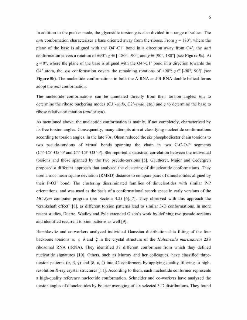
In addition to the pucker mode, the glycosidic torsion χ is also divided in a range of values. The

anti conformation characterizes a base oriented away from the ribose. From χ = 180°, where the

plane of the base is aligned with the O4’-C1’ bond in a direction away from O4’, the anti

conformation covers a rotation of ±90°: χ ! [-180°, -90°[ and χ ! [90°, 180°[ (see Figure 5a). At

χ = 0°, where the plane of the base is aligned with the O4’-C1’ bond in a direction towards the

O4’ atom, the syn conformation covers the remaining rotations of ±90°: χ ! [-90°, 90°[ (see

Figure 5b). The nucleotide conformations in both the A-RNA and B-RNA double-helical forms

adopt the anti conformation.

The nucleotide conformations can be annotated directly from their torsion angles: θ0-4 to

determine the ribose puckering modes (C3’-endo, C2’-endo, etc.) and χ to determine the base to

ribose relative orientation (anti or syn).

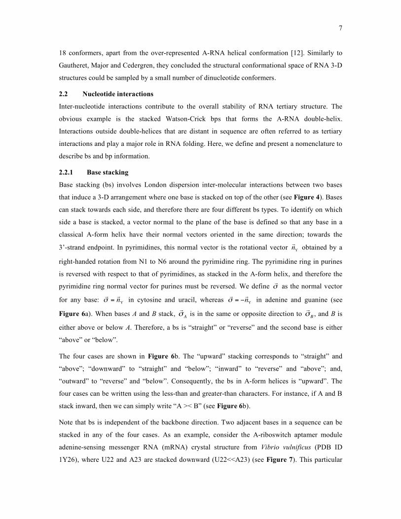
As mentioned above, the nucleotide conformation is mainly, if not completely, characterized by

its free torsion angles. Consequently, many attempts aim at classifying nucleotide conformations

according to torsion angles. In the late 70s, Olson reduced the six phosphodiester chain torsions to

two pseudo-torsions of virtual bonds spanning the chain in two C-C-O-P segments

(C4’-C5’-O5’-P and C4’-C3’-O3’-P). She reported a statistical correlation between the individual

torsions and those spanned by the two pseudo-torsions [5]. Gautheret, Major and Cedergren

proposed a different approach that analyzed the clustering of dinucleotide conformations. They

used a root-mean-square deviation (RMSD) distance to compare pairs of dinucleotides aligned by

their P-O3’ bond. The clustering discriminated families of dinucleotides with similar P-P

orientations, and was used as the basis of a conformational search space in early versions of the

MC-Sym computer program (see Section 4.2) [6],[7]. They observed with this approach the

“crankshaft effect” [8], as different torsion patterns lead to similar 3-D conformations. In more

recent studies, Duarte, Wadley and Pyle extended Olson’s work by defining two pseudo-torsions

and identified recurrent torsion patterns as well [9].

Hershkovitz and co-workers analyzed individual Gaussian distribution data fitting of the four

backbone torsions α, γ, δ and ζ in the crystal structure of the Haloarcula marismortui 23S

ribosomal RNA (rRNA). They identified 37 different conformers from which they defined

nucleotide signatures [10]. Others, such as Murray and her colleagues, have classified three-

torsion patterns (α, β, γ) and (δ, ε, ζ) into 42 conformers by applying quality filtering to high-

resolution X-ray crystal structures [11]. According to them, each nucleotide conformer represents

a high-quality reference nucleotide conformation. Schneider and co-workers have analyzed the

torsion angles of dinucleotides by Fourier averaging of six selected 3-D distributions. They found

7

18 conformers, apart from the over-represented A-RNA helical conformation [12]. Similarly to

Gautheret, Major and Cedergren, they concluded the structural conformational space of RNA 3-D

structures could be sampled by a small number of dinucleotide conformers.

2.2 Nucleotide interactions

Inter-nucleotide interactions contribute to the overall stability of RNA tertiary structure. The

obvious example is the stacked Watson-Crick bps that forms the A-RNA double-helix.

Interactions outside double-helices that are distant in sequence are often referred to as tertiary

interactions and play a major role in RNA folding. Here, we define and present a nomenclature to

describe bs and bp information.

2.2.1 Base stacking

Base stacking (bs) involves London dispersion inter-molecular interactions between two bases

that induce a 3-D arrangement where one base is stacked on top of the other (see Figure 4). Bases

can stack towards each side, and therefore there are four different bs types. To identify on which

side a base is stacked, a vector normal to the plane of the base is defined so that any base in a

classical A-form helix have their normal vectors oriented in the same direction; towards the

3’-strand endpoint. In pyrimidines, this normal vector is the rotational vector Ynr

obtained by a

right-handed rotation from N1 to N6 around the pyrimidine ring. The pyrimidine ring in purines

is reversed with respect to that of pyrimidines, as stacked in the A-form helix, and therefore the

pyrimidine ring normal vector for purines must be reversed. We define !r as the normal vector

for any base: Ynrr

=! in cytosine and uracil, whereas Ynrr

!=" in adenine and guanine (see

Figure 6a). When bases A and B stack,

!

r " A

is in the same or opposite direction to

!

r " B

, and B is

either above or below A. Therefore, a bs is “straight” or “reverse” and the second base is either

“above” or “below”.

The four cases are shown in Figure 6b. The “upward” stacking corresponds to “straight” and

“above”; “downward” to “straight” and “below”; “inward” to “reverse” and “above”; and,

“outward” to “reverse” and “below”. Consequently, the bs in A-form helices is “upward”. The

four cases can be written using the less-than and greater-than characters. For instance, if A and B

stack inward, then we can simply write “A >< B” (see Figure 6b).

Note that bs is independent of the backbone direction. Two adjacent bases in a sequence can be

stacked in any of the four cases. As an example, consider the A-riboswitch aptamer module

adenine-sensing messenger RNA (mRNA) crystal structure from Vibrio vulnificus (PDB ID

1Y26), where U22 and A23 are stacked downward (U22<<A23) (see Figure 7). This particular

8

stacking interaction occurs at a junction that connects two fragments inside the adenine-sensing

pocket. Both U22 and A23 participate in base triples (a base simultaneously pairs to two other

bases) [13].

MC-Annotate implements bs as in Gabb and co-authors [14], by using the distance between the

ring centres, and the dihedral angle and horizontal shift between the rings. As purines are made of

two rings, the pyrimidine and imidazole, both are verified. The bs interactions are labelled

according to the nomenclature above. Note that biased cut-offs on each parameter are needed to

decide whether two bases stack.

2.2.2 Base pairing

Base pairing (bp) involves the formation of hydrogen bonds (HBs) between exocyclic hydrogen

donor groups (mainly NH and NH2) and acceptor groups (mainly CO and N). The well-known

canonical Watson-Crick G=C and A-U bps have three and two HBs, respectively. Successive

Watson-Crick bps that stack upward result in the A-form helix, also called stem (see Figure 4).

The determination of the helices of an RNA from sequence data is the goal of secondary structure

prediction (see Chapter 14). Because stems have a tight and local 3-D structure, they are often

manipulated as rigid objects in computer modeling. Other than Watson-Crick bps abound in

RNAs; near 20% in the yeast phenylalanine transfer (tRNA-Phe) and near 50% in the large

ribosomal subunit), and are often qualified as “non-canonical”, or non Watson-Crick.

In his famous 1984 book, Saenger compiled 28 bp patterns involving at least two HBs [17]. Each

bp was assigned a roman number: for instance XIX for the G=C Watson-Crick bp, XX for the

A-U Watson-Crick bp, XXIII for the “Hoogsteen” A-U bp, XXIV for the “reverse Hoogsteen”

A-U bp, XI for the “sheared” G-A bp; see the book at page 120 for the complete list.

More recently, Leontis and Westhof proposed a new nomenclature, LW [18]. In LW, three HB

contact edges (W: Watson-crick, H: Hoogsteen, and S: Sugar) were defined in each base (see

Figure 8). To describe a bp, one has simply to name its interacting edges. For the Watson-Crick

bp, since the HBs are formed by chemical groups on the W edges of each base, we refer to it as

W/W. In addition, the relative orientation of the riboses with respect to the plane of the bp is

annotated as cis or trans, respectively if the glycosidic bonds extend towards the ribose are in the

same (as in the A-form helix) or opposite orientation (see Figure 9a).

To introduce more precision and distinguished among possible ambiguities of the LW, and in

particular in one-HB bps, Lemieux and Major divided each contact edge in three regions they

named faces [19]. In this extension of LW, LW+, each possible HB face is named by its

9

corresponding LW edge, to which one of three possible orientations was added: w, h and s. For

instance, the W edge has the Ww (or simply W) face at the centre of the edge, the Wh face

towards the H edge, and the Ws face towards the S edge (see Figure 8). The Wobble GU bp is

annotated W/W in LW, and more precisely Ww/Ws in LW+. Bifurcated HBs that oscillate

between two LW edges have their own faces in LW+: Bh between W and H edges, and Bs

between W and S edges.

Finally, the normal vector !r used to annotate base stacking can also be used in base pairing to

address the relative orientation (parallel or antiparallel) of the two bases in a bp. The cis W/W bps

in the A-form helix are characterized by the antiparallel orientation (see Figure 9b).

In order to limit the bias of using cut-offs, Gendron, Lemieux and Major, in MC-Annotate,

implemented the detection of the bp types by using unsupervised learning [19]. Single HBs are

selected by Gaussian distribution fitting of three geometric parameters calculated between all

pairs of bases: the hydrogen, the donor, the acceptor, and lone electron pair (positioned at 1 Å

away from the acceptor in the direction of the orbital). The subset of HBs between two bases are

selected by solving the equilibrium state of the maximal flow of the directed bipartite graph

formed by all possible HBs between the two bases. The bp is labelled according to the LW+

nomenclature. The relative orientations of the glycosidic bonds (cis or trans) and of the normal

vectors (parallel or antiparallel) are also computed. The RNAView annotation procedure of bps

differs considerably from the one implemented in MC-Annotate, as it is based on geometrical cut-

offs.

Lee and Gutell proposed an alternative topological nomenclature, LG. Starting with the Watson-

Crick C=G or A-U, or even with the wobble G-U bp, they defined 14 families by successively

manipulating the base plane and glycosidic bond relative orientations: shearing, flipping,

reversing, paralleling or slipping. The resulting 14 families are the Watson-Crick (WC), wobble

(Wb), slipped Watson-Crick (sWC), slipped wobble (sWb), reversed Watson-Crick (rWC),

reversed wobble (rWb), Hoogsteen (H), reversed Hoogsteen (rH), sheared (S), reversed sheared

(rS), flipped sheared (fS), parallel flipped sheared (pfS), parallel sheared (pS) and reversed parallel

sheared (rpS) [20].

2.2.3 Isosteric base pairs

Bps are isosteric if they preserve a local tertiary structure and, thus, function, as observed in

evolutionary related RNAs whose sequences may diverge. Leontis, Stombaugh and Westhof have

superimposed the geometry of all possible bps according to their C1’-C1’ distances and cis/trans

base orientations [21]. Then, they mapped all sixteen combinations to the twelve families of the

10

LW nomenclature, which resulted in isostericity matrices from which it can be shown that all

canonical Watson-Crick combinations are isosteric, and that the wobble G-U bp is isosteric to the

protonated A-C bp. Walberer, Cheng and Frankel defined isostericity from a theoretical analysis

[22]. They generated a bp database for all possible HB arrangements and deduced an isostericity

measure based on glycosidic bond overlap. They observed high isostericity values in helical bps,

validating their approach, and more surprisingly in several purine-purine and pyrimidine-

pyrimidine combinations.

Accurate RNA sequence comparison requires precise (structural) alignments in order to ensure

the positions compared truly correspond in the tertiary structure. Including isosteric information

in sequence alignment gives better insights into the sequence requirement of structural motifs (see

Section 3) across RNA phylogenies [23]. The presence of isosteric bps is another fact that

supports a rather structural than sequential RNA evolution.

3 MOTIF DISCOVERY

In the previous section, we presented a series of nomenclature and formalisms to describe some

already acknowledged components of RNA tertiary structure: the nucleotide conformations and

interactions. Here we take one step beyond and describe higher-order RNA components.

The increase in high-resolution X-ray crystallographic structures, and in particular the resolution

of the large ribosomal subunit [24][25][26], has increased the literature describing repeated RNA

fragments, or motifs [27]. Many occurrences of each of these fragments can be found in one or

among several different 3-D structures, are conserved among evolutionary related RNAs, and are

often related to specific structural and biochemical functions.

One can think of RNA motifs as RNA fundamental building blocks. Therefore, finding and

characterizing all of them should provide us with invaluable knowledge about RNA folding and

aid substantially in tertiary structure prediction. Here, we present some classical RNA motifs and

introduce a formal definition allowing us to computationally represent, search, and discover them.

3.1 RNA Motifs

The most obvious RNA motif is the double-helix, which is composed of a succession of stacked

Watson-Crick bps. Similarly to the double-helix, RNA motifs are thermodynamically stable and

fold into similar tertiary structures that can be found in various structural contexts.

Let us define an RNA motif as a graph of nucleotide conformations and interactions, where the

nucleotides are the vertices of the graph. An arc between two nucleotides is present if the two

nucleotides are adjacent in the sequence or if their bases interact. Note that if we use the

11

nomenclature introduced in the previous section, then this definition is equivalent to our formal

representation of an annotated RNA tertiary structure; and is in fact the output of the

MC-Annotate computer program.

While RNA graphs are easily represented in computer programs by classical data structures, there

is currently no consensus in the RNA ontology nor is there a data file format to represent them.

RNA graphs in computer programs such as MC-Annotate are serialized into opaque binary files

using the C++ MC-Core library developed in our laboratory (also freely available at

sourceforge.net/projects/mccore). The RNAML format, derived from XML (extensible markup

language), can handle RNA graphs and is portable among many different RNA applications

[28][29].

Since RNA motifs can be represented by characteristic RNA graphs, they can be searched within

hosting RNA tertiary structures via graph isomorphism; the occurrences of an RNA motif are

simply the isomorphic sub-graphs in the hosting graphs. Our laboratory implemented the classical

graph isomorphism algorithm [30] in a computer program called MC-Search. The input to

MC-Search is a description of the target RNA structure, or pattern, from which MC-Search

returns all occurrences of the target motif found in a set of pre-selected PDB files.

3.1.1 Classical examples

Consider the sarcin/ricin motif (Figure 10), which has been predicted to occur in many different

locations of the large ribosomal subunit by comparative sequence analysis [31]. The MC-Search

descriptor file for the sarcin/ricin motif is shown in Figure 10b. MC-Search finds seven

occurrences of this motif in the crystal structure of the Haloarcula marismortui 23S rRNA (PDB

ID 1JJ2). All occurrences found share a maximum RMSD of 0.93 Å. Interestingly, the annotation

of the found occurrences revealed four conserved base stacking interactions (see Figure 10c),

including those among non-adjacent nucleotides: AX1 <> UX3 (outward), GX2 >< GY1 (inward) and

AX4 <> AY2 (outward). Here, the two strands involved in the motif were arbitrarily named X and

Y, and their nucleotides numbered, respectively, 1 to 4 and 1 to 3.

A motif corresponding to the T-loop conserved across tRNAs was matched in the ribosome. In

tRNAs, the loop capping the T stem is characterized by a trans W/H U-A bp stacked on the last

W/W G=C bp of the stem with a two or three nucleotide bulge on the A side. Several instances of

the motif where found by visual inspection in H. marismortui 23S and in Thermus thermophilus

16S subunits [32]. These tRNA T-loop motifs in the ribosome were found to interact with other

elements of their rRNA through tertiary interactions, similarly to the interactions found between

12

the T- and the D-loop in tRNAs. Two instances of the two-nucleotide bulge version are found by

MC-Search in the H. marismortui 23S subunit (Figure 11).

The frequently observed A-minor motif [33] is made of an adenine that interacts with the minor

groove of a double-helix, and is of particular interest since it is involved in the selection of tRNAs

by the ribosome [34]. Nine instances of the A-minor motif are found by MC-Search in the H.

marismortui 23S subunit (Figure 12). Note that the S edge in the bp annotation of the double-

helix nucleotide indicates the minor groove interaction. The A-minor motif is a key element of

the larger K-turn motif which induces a bend between two double-helices [35]. The core of the K-

turn motif is constituted of two S/H G-A bps. There is only one occurrence of the K-turn motif in

the H. marismortui 23S subunit (Figure 13).

The tetraloop/receptor motif is most frequent in RNAs. It stabilizes the conformation of a hairpin

loop interacting with the minor groove of a stem. It was discovered in the hammerhead ribozyme

[36] and in the group I intron [37]. The tetraloop/receptor participates in protein translation

fidelity and in the association of the rRNA 16S and 30S subunits, as mutations in the motif induce

loss of ribosomal activity [38]. In T. thermophilus rRNA, a conserved GCAA tetraloop (refereed

to as loop 900), caps helix 27 in the 16S subunit and binds to the minor groove of helix 24 in the

30S subunit. Two occurences of the tetraloop/receptor motif binding stems of at least three W/W

bps are found by MC-Search in the H. marismortui 23S subunit (Figure 14). Interestingly, the

two occurrences found have different bp orientations.

As found in many pathogenic viruses, the formation of a pseudoknot motif in mRNAs may

induce frameshifting in the protein translation [39][40]. The pseudoknot is made of a hairpin

stem-loop whose nucleotides in the loop participate in the formation of a second stem. In fact, a

pseudoknot occurs when the four strands, A5’, A3’, B5’, and B3’, involved in the formation of

two stems, A and B, interleave in the sequence: A5’-B5’-A3’-B3’. Pseudoknots are reported by

the MC-Annotate computer program, and fifteen are found in the crystal structure of the H.

marismortui 23S rRNA (PDB ID 1JJ2). In the feline immunodeficiency virus (FIV), a

pseudoknot was found by comparative sequence and mutagenesis analyses [41]. The secondary

and tertiary structures of the FIV pseudoknot are shown in Figure 15. See in Section 4.3.2 how

Fabris and his collaborators combined mass spectroscopy and computer modeling to determine

the FIV pseudoknot tertiary structure [42].

3.2 Catalytic motifs

The structure and function of catalytic RNAs (ribozymes) have extensively been studied [43]-

[51]. In particular, the crystal structure of the hammerhead ribozyme shows a three-way junction

13

catalytic core [45]. The three-way junction motif is made of three double-helices, and its topology

has been much studied by Lescoute and Westhof [52]. Interestingly, the H/H and S/S loop-loop

interactions involved in the catalytic mechanism of the hammerhead have been characterized by

3-D modeling by Massire and Westhof, using their computer program MANIP [53][54].

Another relationship between the structure and catalytic activity of RNAs was discovered in the

Neurospora Varkud Satellite (VS) ribozyme. Six helical domains characterize the secondary

structure of the self-cleaving VS ribozyme (see Figure 16a). The substrate domain at stem-loop I

is recognized by the catalytic core by, so far, unknown loop-loop interactions between stem-loop

I and V [55]. The cleavage mechanism of this ribozyme is induced by a modification of the bp

registry in stem I (see Figure 16bc). C637 is paired to G623 in the active state, reducing the size of

the 3’ strand of the internal loop from three to two.

To get a deeper insight into the 3-D structure of the VS ribozyme active conformation, a nuclear

magnetic resonance (NMR) spectroscopy structure of a stem-loop I mutant (SL1’) was built to

mimic the active conformation [56]. In previous NMR structures of the inactive stem-loop I, the

3-3 internal loop was composed of three stacked bps, two S/H G-A and a wobble A-C bps. In the

SL1’ active structure, the A-C bp is broken by the helix shift, resulting in a double S/H bp shared

between both As on the 5’ strand and the G on 3’ strand (see Figure 16c).

This distinctive internal loop motif was searched in other RNAs with the MC-Search computer

program without any specific interaction types in the loop, by using the “pairing” keyword. The

pattern matched a fragment in helix 44 of the T. thermophilus 16S rRNA, which is at 1.4 Å of

RMSD to the NMR structure of the interior loop of SL1’ (see Figure 17). Helix 44 in the rRNA

interacts with helix 13 to form a ribose zipper motif [57], which is defined by ribose-ribose

interactions and the presence of the A-minor motif. Both adenines share one sheared (S/H) G-A

bp. The SL1’ structure became a model for the active substrate element of the VS ribozyme,

which can bind to another helix and form a ribose zipper motif. Since the catalytic mechanism is

characterized by tertiary interactions between stem loop I and V (see Figure 16a), the authors

suggest that the specific interaction needed for an accurate recognition of the substrate is this

ribose zipper.

3.3 Transport and localization

A joint effort between Chartrand’s laboratory in Montreal and our group resulted in a deeper

understanding of the molecular basis behind cytoplasmic mRNA transport and localization to the

yeast bud [58]. A small RNA motif was found conserved across four localization elements within

14

the mRNA of the ASH1 protein. The motif was found to interact with She2p, one of the important

components of the yeast mRNA localization machinery in Saccharomyces cerevisiae.

Three localization elements occur in the coding region (E1, E2A and E2B) [59] and the fourth is

located in the 3’ untranslated region (E3) [60]. Conserved nucleotides in each element were

identified by in vivo selection from a PCR library. Similar She2p RNA motif-binding sites were

characterized, and their secondary structures predicted. The generalized motif is composed of two

loops, separated by a short stem, which contains a conserved C on the 3’ strand and a CGA

sequence on the 5’ strand (see Figure 18), but for E3 for which the loops are inversed.

A structural rule of the generalized She2p-binding motif was deduced: i:s:j, where i is the number

of nucleotides in the loop before the conserved CGA sequence (cf. 1 in the 5’ loop of E1:

GCGAAGA), j the number of nucleotides before the conserved C in the 3’ loop (cf. 1 in the 3’

loop of E1: ACCCAAC), and s the length of the stem separating the two loops (cf. 4 in E1). The

localization element E1 is thus a 1:4:1 motif, E2A and E2B are 2:4:0, and E3 is a 0:5:1. The sum

i+s+j = 6 is invariant.

To find a structural explanation of the invariant rule, MC-Search was used to scan the high-

resolution RNA 3-D structures to seek occurrences of these three types of She2p-binding motifs

(see Figure 19). 123 matches were found for type 1:4:1 (E1), 85 for type 2:4:0 (E2A/E2B) and

717 for type 0:5:1 (E3). The distance between the 3’ phosphate groups of the two conserved

cytosines in all occurrences was 28.3 ± 0.9 Å for type 1:4:1, 28.0 ± 1.0 Å for type 2:4:0 and

28.2 ± 0.7 Å for type 0:5:1. Increasing the length of the She2p-binding motif stem in each

localization elements in the yeast three-hybrids assay resulted in a total loss of interaction with

She2p.

The resolution of the X-ray crystal structure of She2p revealed a helical region essential for its

interaction with ASH1 mRNA localization elements. This helical region covers a distance of

about 27 Å. It was thus logical to the authors to propose a model of the ASH1 mRNA localization

element motif binding to this region of the protein through interactions between the two

conserved Cs. An interesting conclusion from this project is that tertiary structure conservation of

the RNA motif is more relevant to the binding function than sequence conservation.

4 MODELING

In the previous sections, we introduced an ontology to model RNA tertiary structure components

and motifs. Here we employ the term “modeling” to describe 3-D model building. Two types of

3-D models exist: physical or handicraft models (wood, plastic, metal or any other artistic

15

materials) and computer models (interactively built or directly generated). Often, scientists start

with the former type, mainly to draft ideas and to get a global picture of the RNA tertiary

structure, and then, when enough structural data are gathered, they switch to the latter.

The goal of RNA tertiary structure modeling is to summarize and project in 3-D structural data. In

the last few decades, many low-resolution techniques, for instance footprinting, and enzymatic

and chemical probing, have improved and produced a large quantity of structural data.

Consequently, RNA tertiary structure modeling has become very popular and useful in the 90’s to

translate these structural data in precise 3-D models. The low-resolution techniques compensate

when higher-resolution ones cannot be applied, for instance in the case of in vivo or reactive

conformations.

In this Section, we focus on computer assisted model building. There are two major approaches to

3-D modeling. The first one starts with all nucleotides in an extended or randomized state, which

is then successively modified until a folded and satisfactory state is reached. The conformational

space of such folding methods is defined by the number of accessible states. For instance,

molecular mechanics is a folding method that defines satisfaction as the optimum of an objective

function. Harvey’s laboratory has developed an RNA objective function composed of penalty

terms corresponding to experimentally determined nucleotide interactions and distances. The

objective function is penalized if the observed interactions and distances are not present in a state.

They simplified the RNA model by using one to five points per nucleotide to speedup the folding

operations. Using YAMMP, their computer program, they were able to build models of large

ribosomal subunits [61]. In the second approach, one assembles the components of the RNA by

using construction operators to position and orient them in 3-D space. MANIP [54], an interactive

system, and MC-Sym [62], an automated procedure, are among the most employed computer

systems to model RNA tertiary structures.

In this section, we present how RNA tertiary structure modeling can be mapped to the discrete

constraint satisfaction problem (CSP) and how the CSP solver was implemented in the MC-Sym

computer program.

4.1 The CSP (Constraint Satisfaction Problem)

The CSP can be described by three finite sets: the variables V = {v1, v2, …, vn}, the domains

D = {d1, d2, …, dn} and the constraints C = {c1, c2, …, cm} [63][64]. A variable vi is assigned

values from domain di = {di,1, di,2, …, di,|di|}. Each constraint restricts the assignment of a subset

16

of V, called the constraint scope. For example, if the scope of c1 ∈ C is {v2, v4, v5} ⊂ V, then

c1 ⊂ d2 × d4 × d5.

The three sets are defined in the context of the problem application. In RNA tertiary structure

prediction, the variables could be the nucleotides and the domains their possible 3-D coordinates.

An example of constraint would be two nucleotides that form a bp. The scope of the bp constraint

is the two nucleotide partners which link their relative positions and orientations in 3-D space.

A solution to the CSP is a complete variable assignment, vi ∈ di for i ∈ {1…n}, so that all

constraints in C, cj ∈ C for j ∈ {1…m} are satisfied. A constraint cj is satisfied only if its scope in

the solution is assigned according to the relation it defines. Solving the CSP consists in finding

one, many or all solutions.

The search space of a CSP is the Cartesian product of all di:

!=

n

i

id

1

(4)

The size of a CSP search space is exponential in the number of variables domain sizes. The

solutions of a CSP are found by exploring the variable assignments of its search space and

verifying if they satisfy the constraints. Backtracking is the classical search algorithm to solve a

CSP deterministically and exhaustively. In backtracking, the variables are assigned values

systematically, one at a time and to the next available value from its associated domain. When all

the values of a domain have been tried, the domain is reset and backtracking moves to the

previous variable, assigning its next value, before continuing. The search finishes when the

domain of the first variable is reset, indicating that all possible assignments have been tried.

Backtracking develops a search tree (see Figure 20), where the nodes are visited in a depth-first

manner. A path from the root of the search tree to a leaf represents a solution if all of its nodes are

consistent (the black nodes in Figure 20). The search tree size is given by Equation 5:

!"= =

+n

i

i

j

id

1 1

1 (5)

However, the search can avoid visiting most inconsistent nodes by pruning from the search tree

inconsistent branches (those with grey nodes in Figure 20), as soon as one inconsistent node is

found. This trick does not change the search time complexity of backtracking, which is

exponential in n and |di|, but can reduce the search time in practice. Using MC-Sym (see next

section), the search space of a particular instance of the CSP for the yeast tRNA-Phe tertiary

17

structure was 1026, but the constraints used to explore it defined a consistent search tree of only

about 5 × 105, which was explored in seconds and included only about 30 solutions [65]. The best

model was at approximately 3.0 Å of RMSD to the yeast tRNA-Phe, as well as with the yeast

tRNA-Asp crystal structures (crystal structure resolution). In RNA tertiary structure prediction, it

is customary to assess the quality of a prediction method by evaluating its performances at

refolding known structures, and RMSD is a very popular quantitative measure.

4.2 MC-Sym

MC-Sym (Macromolecular Conformations by SYMbolic programming) is a computer program

for building RNA tertiary structure models from syntactic descriptions of the RNA, similar to the

ones used for MC-Search. The computer program implements a CSP solver with backtracking,

and thus generates models that are consistent with the constraints [6][62][65][66].

In MC-Sym, the variables, V, correspond to the vertices, v, and arcs, a, of the RNA graph (see

Section 3.1). The domains of the vertices, Dv, are rigid nucleotides (the relative 3-D atomic

coordinates never change), and those of the arcs, Da, are linear transformation matrices encoding

bs and bp. Consequently, the domains, D, are taken from the Cartesian product, D = Dv X Da. The

goal is to generate consistent and 3-D atomic coordinates to each nucleotide in the global frame

of the RNA. The rigid sets of nucleotide 3-D atomic coordinates, as well as the linear

transformation matrices, are extracted from the PDB [1]. The nucleotide is defined by cutting the

phosphodiester chain at the O3’-P bond.

The linear transformation matrices combine nucleotide rotations and translations in 4-D

homogeneous coordinates, which represent the spatial relation between two stacked or paired

bases. As we saw in Section 2.2, nucleotide interactions involve their bases, and thus we represent

their spatial relations by coordinate frame relative transformations. The frames are defined at the

terminal nitrogen atom (N9 in purines and N1 in pyrimidines), with the XY plane aligned with the

base plane (see Figure 21ab).

For any coordinate frames A and B, the relative transformation AMB expresses B’s position (right

subscript) in A’s coordinates (left superscript). For example, let AMB be a relative transformation

that expresses a stacking interaction between an adenine (frame A) and a cytosine (frame B).

Because the relative transformation AMB is defined in A’s frame, B can be moved from a position

aligned on A’s frame to a position that expresses the stacking interaction between the two bases

(Figure 21c). This relative transformation places B in the local frame of A, independently of A’s

position in the global frame. Then, to obtain B’s position in the global frame, O, it must be

transformed by the relative matrix OMA, which expresses A’s position in the global frame.

18

Using such transformations, all nucleotides of an RNA graph can be positioned relatively to

another by starting with an initial origin nucleotide, which frame defines the global frame, O. A

construction order is defined by selecting a spanning tree of the RNA graph rooted at the origin

nucleotide. The transformations of the arcs of the spanning tree applied to the rigid coordinates of

the vertices build the RNA (see Figure 22). Ideally, the chosen spanning tree of the RNA graph

would include all arcs. However, RNA graphs are rarely trees1, as they include cycles of

interactions. Consequently, the missing arcs must be represented by constraints in the CSP, C. As

we will see in Section 4.3.3, this problem can be overcome.

The search space for an RNA tertiary structure prediction problem defined with this instance of

the CSP is given by the spanning tree n nucleotide variables and n-1 interactions. Equation 6

gives the size of the search space, the Cartesian product Dv X Da, where xi ∈ Dv , yi ∈ Da.

!

xii=1

n

" # yii=1

n$1

" (6)

Two types of constraints need to be verified at each variable assignment: the atomic clashes and

the O3’-P covalent bond distances. The scope of the atomic clash constraints is all nucleotide

pairs, and they are needed to insure that any pair of atoms from both nucleotides is not

overlapping. A threshold inter-atomic distance, typically 1 Å, implements the steric clash

constraints.

The adjacency constraint, as we name it, has a scope of two adjacent nucleotides in the sequence

and is used to verify the covalent O3’-P bond distance (dashed lines in Figure 22b), as the

nucleotide backbone are positioned independently. The distance threshold is fixed by a user

distance range, typically set to [1, 2] Å, as the O-P theoretical distance is approximately 1.6 Å

(see Section 4.3). Note that choosing a lower bound smaller that the atomic clash threshold would

be useless. Increasing the upper bound is equivalent to “relaxing” the CSP. If an overstretched

backbone results from choosing a high upper bound, it can easily be fixed by applying numerical

refinement [6].

1 The only situation where a RNA graph is a tree is when the only information available is the sequence.

19

4.2.1 Backbone optimization

In the above mapping of the RNA tertiary structure CSP, the adjacency constraint is violated

more than 50% of the time, even if its range is relaxed to [1, 5] Å. This problem comes from the

rigid nucleotide conformations that do not reflect well the overall flexibility of the backbone.

To address this problem, we propose a slight modification of the above CSP mapping. We make

the assumption that the RNA tertiary structure is driven by rigid base interactions. Consequently,

the backbone conformation can be derived from the bases, and we can define a new CSP on the

bases alone. The new CSP defines a search space over the transformation matrices, Da, reducing

considerably its size to

!

yii=1

n"1

# (see Equation 6).

To reduce the complexity of building a complete backbone from six free torsion angles (eleven in

total minus the five of the furanose), we define rigid conformations made of the base and the

phosphate group. The ribose interconnects a base with two phosphate groups. To position all of

the ribose atoms, six free torsions are needed: θ0, θ1, θ2, θ3, θ4 and χ (see Figure 3a). But we know

from Equations 1 and 3 that θ0 to θ4 are all related by the single pseudorotation angle ρ (Section

2.1). Hence, by fixing all covalent bond lengths and angles to their theoretical values, a ribose

structure can be built by optimizing a suitable function, f (ρ, χ). f builds a ribose using torsions ρ

and χ and returns the RMSD between the theoretical and the implicit values of the C5’-O5’ and

C3’-O3’ bonds (see Figure 23). Equation 7 gives the value of f (ρ, χ), where lk are the measured

distances and λk are the theoretical distances, k = 5’ or k = 3’ respectively for the C5’-O5’ or the

C3’-O3’ bond.

( )( ) ( )

2,

2

'3'3

2

'5'5!!

"#$+$

=ll

f (7)

Finding the optimal parameters (that minimize) Equation 7 builds a ribose attached to its base and

interconnecting phosphate groups. The minimization can be solved using classical optimization

methods, such as the cyclic coordinate method that does not require derivatives [67]. In this

context, each evaluation of the function builds a different ribose conformation. Consequently, the

time complexity is proportional to the number of evaluations needed. However, we recently

derived an optimal parameter estimation of Equation 7, which solves the ribose optimization in

constant time.

Theoretically, the backbone construction can be applied once all variables of the CSP are

assigned values; when all bases and phosphate groups are in place. After the backbone

20

construction, however, there is no guarantee that the final model is free of any steric conflicts.

Therefore, in practice, as soon as the two phosphate groups adjacent to a base are in place, the

backbone is built for this nucleotide and the steric clashes verified. This, as the former

backtracking, allows us to prune the search tree.

4.2.2 Probabilistic backtracking

Exhaustive searches for all valid RNA 3-D structures are useful to analyze possible alternative

foldings of an RNA. However, sometimes only one or few valid models are desired. We recently

developed a probabilistic search algorithm that generates valid structures faster and with an

increased diversity rate than that of the deterministic backtracking.

We select a random path from the root node of the search tree to any leaf. If at any variable

assignment along the random path a constraint is not satisfied, a fixed-size regular backtracking is

run until a consistent node is found, which resumes the probabilistic search. If the fixed-size

regular backtracking cannot find a consistent node, then a new random path from the root node is

selected.

4.2.3 Divide-and-conquer

As for many problems, the “divide and conquer” paradigm has proven useful in RNA tertiary

structure prediction as well. A divide-and-conquer algorithm splits a complex problem in many

smaller and simpler to resolve sub-problems. The solutions of the smaller problems are then

combined in complete solutions of the larger problem.

RNA structures can be split into smaller fragments (as we saw in Section 3). Each fragment can

be built independently, and then merged in complete tertiary structures. In the CSP context,

solving a fragment means locally enforcing the constraints in its scope: solving subset W ⊂ V

involves the verification of the constraints defined on W only. The solutions of W become the

values of the domain of a new variable, say w, which is added to the CSP. The new CSP, CSP’, is

defined over the variables V’ = (V \ W) ∪ {w}, the new domain for w, and the new constraints

C’ = C \ Cw.

The search space sizes of CSP and CSP’ can be compared. Let D = {d1, …, dn} be the domains

for the n variables in V, and as defined in the CSP. E = {e1, …, ek} are the domains for the k

variables in W, E ⊂ D. The domain for the new variable, w, is dw, the solutions of W. If S and S’

are respectively the search space sizes of CSP and CSP’, then from Equation 4 we obtain:

21

!!!

!

==

=

= <"<#"<k

i

iw

n

i

iwk

i

i

n

i

i

eddd

e

d

SS

11

1

1'

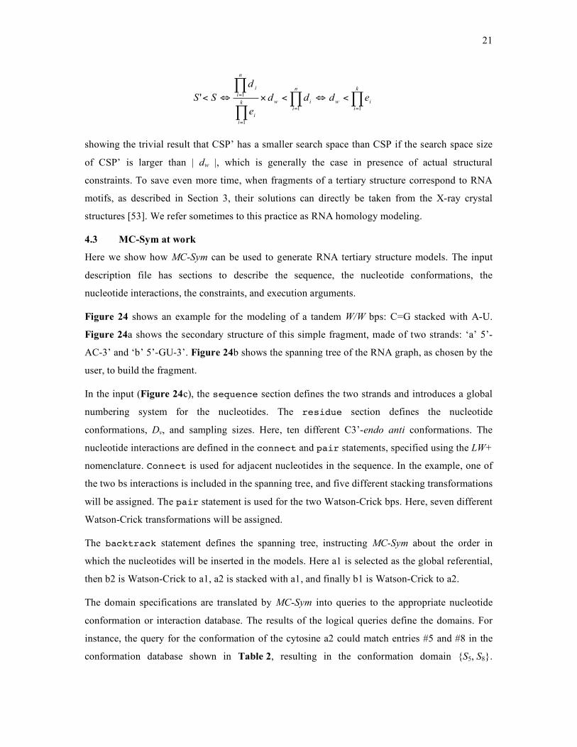
showing the trivial result that CSP’ has a smaller search space than CSP if the search space size

of CSP’ is larger than | dw |, which is generally the case in presence of actual structural

constraints. To save even more time, when fragments of a tertiary structure correspond to RNA

motifs, as described in Section 3, their solutions can directly be taken from the X-ray crystal

structures [53]. We refer sometimes to this practice as RNA homology modeling.

4.3 MC-Sym at work

Here we show how MC-Sym can be used to generate RNA tertiary structure models. The input

description file has sections to describe the sequence, the nucleotide conformations, the

nucleotide interactions, the constraints, and execution arguments.

Figure 24 shows an example for the modeling of a tandem W/W bps: C=G stacked with A-U.

Figure 24a shows the secondary structure of this simple fragment, made of two strands: ‘a’ 5’-

AC-3’ and ‘b’ 5’-GU-3’. Figure 24b shows the spanning tree of the RNA graph, as chosen by the

user, to build the fragment.

In the input (Figure 24c), the sequence section defines the two strands and introduces a global

numbering system for the nucleotides. The residue section defines the nucleotide

conformations, Dv, and sampling sizes. Here, ten different C3’-endo anti conformations. The

nucleotide interactions are defined in the connect and pair statements, specified using the LW+

nomenclature. Connect is used for adjacent nucleotides in the sequence. In the example, one of

the two bs interactions is included in the spanning tree, and five different stacking transformations

will be assigned. The pair statement is used for the two Watson-Crick bps. Here, seven different

Watson-Crick transformations will be assigned.

The backtrack statement defines the spanning tree, instructing MC-Sym about the order in

which the nucleotides will be inserted in the models. Here a1 is selected as the global referential,

then b2 is Watson-Crick to a1, a2 is stacked with a1, and finally b1 is Watson-Crick to a2.

The domain specifications are translated by MC-Sym into queries to the appropriate nucleotide

conformation or interaction database. The results of the logical queries define the domains. For

instance, the query for the conformation of the cytosine a2 could match entries #5 and #8 in the

conformation database shown in Table 2, resulting in the conformation domain {S5, S8}.

22

Similarly, the Watson-Crick query for the a2-b1 interaction could match database entries #1, #3

and #8 in Table 3, resulting in the transformation domain {T1, T3, T8}.

As indicated in Tables 2 and 3, the conformation and transformation domains come from X-ray

crystal structures. The atomic coordinates for the conformations are directly extracted. The

transformation between two nucleotides, A and B, is extracted by computing the relative

transformation that places B’s frame in A’s local frame (Figure 25). If OMA and OMB are

respectively the relative transformations that place the frame of A and B in the global frame, O,

then we extract the relative transformation AMB so that OMB = OMA × AMB. Isolating for AMB, we

obtain AMB = OMA-1 × OMB. We save the AMB matrix in the database so that it can be reproduced

for any other pair of bases in any local frame.

The MC-Sym database contains near 3000 nucleotide conformations and near 20000 base

interactions, hence the domain size argument next to each conformation and interaction. It is the

task of the modeler to assign domain sizes so that the conformational space of a given tertiary

structure is correctly addressed; not too small to miss valid models and not too large to avoid

prohibitive search space sizes.

4.3.1 Modeling a yeast tRNA-Phe stem-loop

In Figure 26, we present a modeling example for the yeast tRNA-Phe T-stem-loop tertiary

structure. The secondary structure of the stem-loop is shown in Figure 26a. The stem and hairpin

loop are modeled independently, and the results of each modeling merged. Figure 26b-d shows

the three inputs. The first describes the structure of the first four bps of the stem. The second

describes the hairpin loop, closed by the last bp of the stem. The last merges the resulting

fragments and, thus, model the entire stem-loop. Figure 26e-g illustrates the spanning trees

defined by the three inputs.

The res_clash and adjacency statements parameterize the steric clashes and adjacency

constraints, respectively. The explore statement launches the CSP solver. The RNA graph of

the loop is divided into two sections by the W/H U54-A58 bp, leaving the sequence adjacency

implicit to the construction between G57 and A58, and between C60 and C61. Figure 26h shows

one solution.

4.3.2 Modeling a pseudoknot

To model the tertiary structure of the FIV pseudoknot (see Section 3.1.1), a novel methodological

protocol based on mass spectroscopy and computer modeling was designed by Fabris and his co-

workers. The experimental data were generated using multiplexing solvent-accessibility probes

23

and chemical bifunctional crosslinkers with a characterization by an electrospray ionization

Fourier transform mass spectrometry method (ESI-FTMS) [68]. The chemical and enzymatic

probes cleave at specific sites or attack specific chemical groups that are exposed to the solvent.

The secondary structure, detailed protection maps, and inter-nucleotide distance information were

then input to MC-Sym, which generated a set of consistent tertiary structures. Finally, the modeled

structures were refined by energy minimization using the Crystallography and NMR System

(CNS) [69].

4.3.3 Cycles of interactions

Traversal of a spanning tree to build tertiary structures implies a conceptual problem, as was

pointed out in Section 4.2. A spanning tree does not cover all the arcs of the RNA graph. User

constraints must be added to the input to make sure the dropped interactions are satisfied.

However, such ad hoc constraints are difficult to define and compute. Lemieux and Major have

designed a novel building approach to decompose an RNA graph in a series of minimum cycles

of interactions, which solutions can be combined by superimposing common arcs. The RNA

graph in Figure 24, for instance, is a minimum cycle of four nucleotides. The product of the four

transformation matrices is the identity matrix, representing an additional constraint to insure the

consistency of the cycle and the satisfaction of the four interactions.

These minimum interaction cycles could well be used as first-class objects in stochastic graph

grammars [70][71] to represent the tertiary structure of related RNAs and of their sequence

alignment. This is similar, but yet more expressive, than stochastic context-free grammars

employed to represent RNA secondary structures [72][73].

5 Perspectives

Accurate prediction of RNA tertiary structures from sequence alone is still an unresolved

problem. In the meantime, formalizing RNA attributes, searching for higher-order levels of

structural organization, and modeling their tertiary structure represent current efforts towards

better understanding of the RNA architectural principles. In addition, formalizing RNA structural

knowledge in computer programs offers the possibility to apply it in a systematic and objective

manner, allowing us to generate new and experimentally testable data.

The recent resolution of several RNA structures by X-ray crystallography, NMR, but also by

computer modeling has allowed us to observe repeated RNA fragments, or motifs, and to infer

their function. We are starting to understand the sequence constraints imposed by the tertiary

structure of these fragments and to discover local and global folding rules. In the coming years, as

24

we can also expect agreement on an RNA ontology (nomenclatures and formalisms), we might

assist in the deployment and implementation of these folding rules into accurate RNA tertiary

structure prediction algorithms. An RNA ontology will enable the interoperability of research

results. Consequently, as we will identify the RNAs of key cellular processes, determine their

structure, and characterize their role, we will be in a better position to manipulate them. As a

result, we should observe an increase in the number and an improvement in the accuracy of RNA-

based molecular medicine techniques.

25

6 Bibliography

[1] Berman, H. M., J. Westbrook, Z. Feng, G. Gilliland, T. N. Bhat, H. Weissig, I. N. Shindyalov and P. E. Bourne. 2000. The Protein Data Bank. Nucleic Acids Res 28:235-242.

[2] Gendron, P., S. Lemieux and F. Major. 2001. Quantitative analysis of nucleic acid three-dimensional structures. J Mol Biol 308:919-936.

[3] Yang, H., F. Jossinet, N. B. Leontis, L. Chen, J. Westbrook, H. M. Berman and E. Westhof. 2003. Tools for the automatic identification and classification of RNA base pairs. Nucleic Acids Res 31:3450-3460.

[4] Altona, C. and M. Sundaralingam. 1972. Conformational analysis of the sugar ring in nucleosides and nucleotides. A new description using the concept of pseudorotation. J Amer Chem Soc 94:8205-8212.

[5] Olson, W. K. 1980. Configurational statistics of polynucleotide chains. An updated virtual bond model to treat effects of base stacking. Macromolecules 13:721-728.

[6] Major, F., M. Turcotte, D. Gautheret, G. Lapalme, E. Fillion and R. Cedergren. 1991. The combination of symbolic and numerical computation for three-dimensional modeling of RNA. Science 253:1255-1260.

[7] Gautheret, D., F. Major and R. Cedergren. 1993. Modeling the three-dimensional structure of RNA using discrete nucleotide conformational sets. J Mol Biol 229:1049-1064.

[8] Paul, R. P. 1981. Robot manipulators: mathematics, programming and control. MIT Press, Cambridge, USA.

[9] Duarte, C. M., L. M. Wadley and A. M. Pyle. 2003. RNA structure comparison, motif search and discovery using a reduced representation of RNA conformational space. Nucleic Acids Res 31:4755-4761.

[10] Hershkovitz, E., E. Tannenbaum, S. B. Howerton, A. Sheth, A. Tannenbaum and L. D. Williams. 2003. Automated identification of RNA conformational motifs: theory and application to the HM LSU 23S rRNA. Nucleic acids Res 31:6249-6257.

[11] Murray, L. J. W., W. B. III Arendall, D. C. Richardson and J. S. Richardson. 2003. RNA backbone is rotameric. Proc Natl Acad Sci USA, 100:13904-13909.

[12] Schneider, B., Z. Morávek and H. M. Berman. 2004. RNA conformational classes. Nucleic Acids Res 32:1666-1677.

[13] Serganov, A., Y. R. Yuan, O. Pikovskaya, A. Polonskaia, L. Malinina, A. T. Phan, C. Hobartner, R. Micura, R. R. Breaker and D. J. Patel. 2004. Structural basis for discriminative regulation of gene expression by adenine- and guanine-sensing mRNAs. Chem Biol 11:1729-1741.

[14] Gabb, H. A., S. R. Sanghani, C. H. Robert and C. Prévost. 1996. Finding and visualizing nucleic acid base stacking. J Mol Graphics 14:6-11.

[15] Kraulis, P. J. 1991. Molscript: a program to produce both detailed and schematic plots of protein structures. J Appl Crystallogr 24:946-950.

[16] Merritt, E. A. and M. E. Murphy. 1994. Raster3D version 2.0. A program for photorealistic molecular graphics. Acta Crystallogr Sect D: Biol Crystallogr 50:869-873.

[17] Saenger, W. 1984. Principles of nucleic acid structure. Springer-Verlag, New York, USA.

26

[18] Leontis, N. B. and E. Westhof. 2001. Geometric nomenclature and classification of RNA base pairs. RNA 7:499-512.

[19] Lemieux, S. and F. Major. 2002. RNA canonical and non-canonical base pairing types: a recognition method and complete repertoire. Nucleic Acids Res 30:4250-4263.

[20] Lee, J. C. and R. R. Gutell. 2004. Diversity of base-pair conformations and their occurrence in rRNA structure and RNA structural motifs. J Mol Biol 344:1225-1249.

[21] Leontis, N. B., J. Stombaug and E. Westhof. 2002. The non-Watson-Crick base pairs and their associated isostericity matrices. Nucleic Acids Res 30:3479-3531.

[22] Walberer, B. J., A. C. Cheng and A. D. Frankel. 2003. Structural diversity and isomorphism of hydrogen-bonded base interactions in nucleic acids. J Mol Biol 327:767-780.

[23] Lescoute, A., N. B. Leontis, C. Massire and E. Westhof. 2005. Recurrent structural RNA motifs, isostericity matrices and sequence alignments. Nucleic Acids Res. 33:2395-2409.

[24] Ban, N., P. Nissen, J. Hansen, P. B. Moore and T. A. Steitz. 2000. The complete atomic structure of the large ribosomal subunit at 2.4 Å resolution. Science 289:905-920.

[25] Wimberly, B. T., D. E. Brodersen, W. M. Jr. Clemons, R. J. Morgan-Warren, A. P. Carter, C. Vonrhein, T. Hartsch and V. Ramakrishnan. 2000. Structure of the 30S ribosomal subunit. Nature 407:327-339.

[26] Harms, J., F. Schluenzen, R. Zarivach, A. Bashan, S. Gat, I. Agmon, H. Bartels, F. Franceschi and A. Yonath. 2001. High resolution structure of the large ribosomal subunit from a mesophilic eubacterium. Cell 107:679-688.

[27] Leontis, N. B. and E. Westhof. 2003. Analysis of RNA motifs. Curr Opin Struct Biol 13:300-308.

[28] Waugh, A., P. Gendron, R. Altman, J. W. Brown, D. Case, D. Gautheret, S. C. Harvey, N. B. Leontis, J. Westbrook, E. Westhof, M. Zuker and F. Major. 2002. RNAML: a standard syntax for exchanging RNA information. RNA 8:707-717.

[29] Jossinet, F. and E. Westhof. 2005. Sequence to structure (S2S): display, manipulate and interconnect RNA data from sequence to structure. Bioinformatics 1:3320-3321.

[30] Ullman, J. R. 1976. An Algorithm for Subgraph Isomorphism. J Assoc Comp Machinery 23:31-42.

[31] Leontis, N. B., J. Stombaugh and E. Westhof. 2002. Motif prediction in ribosomal RNAs. Lessons and prospects for automated motif prediction in homologous RNA molecules. Biochimie 84:961-973.

[32] Nagaswamy, U. and G. E. Fox. 2002. Frequent occurrence of the T-loop RNA folding motif in ribosomal RNAs. RNA 8:1112-1119.

[33] Nissen, P., J. A. Ippolito, N. Ban, P. B. Moore and T. A. Steitz. 2001. RNA tertiary interactions in the large ribosomal subunit: the A-minor motif. Proc Natl Acad Sci USA 98:4899-4903.

[34] Ogle, J. M., F. V. IV Murphy, M. J. Tarry and V. Ramakrishnan. 2002. Selection of tRNA by the ribosome requires a transition from an open to a closed form. Cell 111:721-732.

[35] Klein, D. J., T. M. Schmeing, P. B. Moore and T. A. Steitz. 2001. The kink-turn: a new RNA secondary structure motif. EMBO J, 20:4214-4221.

[36] Pley, H. W., K. M. Flaherty and D. B. McKay. 1994. Model for an RNA tertiary interaction from the structure of an intermolecular complex between a GAAA tetraloop and an RNA helix. Nature 372:111-113.

27

[37] Jaeger, L., F. Michel and E. Westhof. 1994. Involvement of a GNRA tetraloop in long-range RNA tertiary interactions. J Mol Biol 236:1271-1276.

[38] Bélanger, F., M. G. Gagnon, S. V. Steinberg, P. R. Cunningham and L. Brakier-Gingras. 2004. Study of the functional interaction of the 900 tetraloop of 16S ribosomal RNA with helix 24 within the bacterial ribosome. J Mol Biol 338:683-693.

[39] ten Dam, E., C. W. A. Pleij and D. E. Draper. 1992. Structural and functional aspects of RNA pseudoknots. Biochemistry 47:11665-11676.

[40] Giedroc, D. P., C. A. Theimer and P. L. Nixon. 2000. Structure, stability and function of RNA pseudoknots involved in stimulating ribosomal frameshifting. J Mol Biol 298:167-185.

[41] Morikawa, S. and D. H. L. Bishop. 1992. Identification and analysis of the gap-pol ribosomal frameshift site of feline immunodeficiency virus. Virology 186:389-397.

[42] Yu, E. T., Q. Zhang and D. Fabris. 2005. Untying the FIV frameshifting pseudoknot structure by MS3D. J Mol Biol 345:69-80.

[43] Ruffner, D. E., G. D. Stormo and O. C. Uhlenbeck. 1990. Sequence requirements of the hammerhead RNA self-cleavage reaction. Biochemistry 29:10695–10702.

[44] Pley, H. W., K. M. Flaherty and D. B. McKay. 1994. Three-dimensional structure of a hammerhead ribozyme. Nature 372:68–74.

[45] Scott, W. G., J. T. Finch and A. Klug. 1995. The crystal structure of an all-RNA hammerhead ribozyme: a proposed mechanism for RNA catalytic cleavage. Cell 81:991–1002.

[46] Legault, P., C. G. Hoogstraten, E. Metlitzky and A. Pardi. 1998. Order, dynamics and metal-binding in the lead-dependent ribozyme. J Mol Biol 284:325-335.

[47] Lemieux, S, P. Chartrand, R. Cedergren and F. Major. 1998. Modeling active RNA structures using the intersection of conformational space: application to the lead-activated ribozyme. RNA 4:739-749.

[48] Wedekind, J. E. and D. B. McKay. 1999. Crystal structure of a lead-dependent ribozyme revealing metal binding sites relevant to catalysis. Nature Struct Biol 6:261-268.

[49] David, L., D. Lambert, P. Gendron and F. Major. 2001. Leadzyme, in Ribonucleases, Methods in Enzymology. Nicholson, A. W. eds, Academic Press Inc., New York, USA, 341, 518-540.

[50] Pinard, R., D. Lambert, J. E. Heckman, J. A. Esteban, B. Gundlach, G. Click, N. G. Walter, F. Major and J. M. Burke. 2001. The hairpin ribozyme substrate binding domain: A highly constrained D-shaped conformation. J Mol Biol 307:51-65.

[51] Pinard, R., D. Lambert, G. Pothiawala, F. Major and J. M. Burke. 2004. Modifications and deletions of helices within the hairpin ribozyme-substrate complex: an active ribozyme lacking helix 1. RNA 10:395-402.

[52] Lescoute, A. and E. Westhof. 2006. Topology of the three-way junctions in folded RNAs. RNA 12:83-93.

[53] Khvorova, A., A. Lescoute, E. Westhof and S. D. Jayasena. 2003. Sequence elements outside the hammerhead ribozyme catalytic core enable intracellular activity. Nature Struct Biol 10:708-712.

[54] Massire, C. and E. Westhof. 1998. MANIP: an interactive tool for modeling RNA. J Mol. Graphics Mod 16:197-205.

[55] Hiley, S. L. and R. A. Collins. 2001. Rapid formation of a solvent_inaccessible core in the Neurospora Varkud satellite ribozyme. EMBO J 20:5461-5469.

28

[56] Hoffmann, B., G. T. Mitchell, P. Gendron, F. Major, A. A. Andersen, R. A. Collins and P. Legault. 2003. NMR structure of the active conformation of the Varkud satellite ribozyme cleavage site. Proc Natl Acad Sci USA 100:7003-7008.

[57] Tamura, M. and S. R. Holbrook. 2002. Sequence and structural conservation in RNA riboses. J Mol Biol 320:455-474.

[58] Olivier, C., G. Poirier, P. Gendron, A. Boisgontier, F. Major and P. Chartrand. 2005. Identification of a conserved RNA motif essential for She2p recognition and mRNA localization to the yeast bud. Mol Cell Biol 25:4752-4766.

[59] Chartrand, P., X.-H. Meng, R. H. Singer and R. M. Long. 1999. Structural elements required for the localization of ASH1 mRNA and of a green fluorescent protein reporter particle in vivo. Curr Biol 9:333-336.

[60] Long, R. M., W. Gu, E. Lorimer, R. H. Singer and P. Chartrand. 2000. She2p is a novel RNA-binding protein that recruits the Myo4p-She3p complex to ASH1 mRNA. EMBO J 19:6592-6601.

[61] Malhotra, A., R. K. Tan and S. C. Harvey. 1990. Prediction of the three-dimensional structure of Escherichia coli 30S ribosomal subunit: a molecular mechanics approach. Proc Natl Acad Sci USA 87:1950-1954.

[62] Major, F. 2003. Building three-dimensional ribonucleic acid structures. IEEE Computing in Science and Engineering sept.-oct. 2003:44-53.

[63] Hentenryck, P. V. 1989. Constraint Satisfaction in Logic Programming. The MIT Press, Cambridge, USA.

[64] Dechter, R. and D. Frost. 2002. Backjump-based backtracking for constraint satisfaction problems. Artificial Intelligence 136:147-188.

[65] Major, F., D. Gautheret and R. Cedergren. 1993. Reproducing the three-dimensional structure of a tRNA molecule from structural constraints. Proc Natl Acad Sci USA 90:9408-9412.

[66] Lemieux, S., S. Oldziej and F. Major. 1998. Nucleic acids: qualitative modeling, in Encyclopedia of Computational Chemistry. Schleyer, P. v. R., N. L. Allinger, T. Clark, J. Gasteiger, P. A. Kollman, H. F. III Schaefer and P. R. Schreiner eds., John Wiley & Sons, West Sussex, UK.

[67] Bazaraa, M. S. and C. M. Shetty. 1979. Nonlinear Programming theory and algorithms. John Wiley & Sons, New York, USA.

[68] Yu, E. T. and D. Fabris. 2003. Direct probing of RNA structures and RNA-protein interactions in the HIV-1 packaging signal by chemical modification and electrospray ionization Fourier transform mass spectrometry. J Mol Biol 330:211-223.

[69] Brünger, A.T., P. D. Adams, G. M. Clore, W. L. DeLano, P. Gros, R. W. Grosse-Kunstleve, J. S. Jiang, J. Kuszewski, M. Nilges, N. S. Pannu, R. J. Read, L. M. Rice, T. Simonson and G. L. Warren. 1998. Crystallography & NMR system: a new software suite for macromolecular structure determination. Acta Crystallogr Sect D: Biol Crystallogr 54:905-921.

[70] Nagl, M. 1987. Set theoretic approaches to graph grammars, in Graph-grammars and their application to computer science. Ehrig, H., M. Nagl, G. Rozenberg and A. Rosenfeld eds, Springer-Verlag, Berlin, 41-54.

[71] Jones, C. V. 1993. An integrated modeling environment based on attributed graphs and graph-grammars. Decision Support Systems 10:255-275.

29

[72] Sakakibara, Y., M. Broen, R. Hughey, I. S. Mian, K. Sjölander, R. C. Underwood and D. Haussler. 1994. Stochastic context-free grammars for tRNA modeling. Nucleic Acids Res 22:5112-5120.

[73] Dowell, R. D. and S. R. Eddy. 2004. Evaluation of several lightweight stochastic context-free grammars for RNA secondary structure prediction. BMC Bioinformatics 5:71.

30

7 Figure legends

Figure 1. Data flow and research activities of tertiary structure prediction. Structural data are used to develop the (computational) tools employed by the researchers to annotate, inspect and model RNA tertiary structures. Structural hypotheses are generated and, challenged experimentally, bring new structural data to research.

Figure 2. RNA chemical structure. The polynucleotide chain (on the left) is made of the bases (hexagons), riboses (pentagons), and phosphate groups (diamonds). The four common types of bases (on the right): the two purines adenine and guanine, and the two pyrimidines cytosine and uracil. The phosphodiester linkage (middle) connects two nucleotides. The ribose (center) links two phosphate groups: one to its 5’ oxygen (above) and the other to its 3’ oxygen (below). The conventional atomic numbering system is used. Small black circles represent the carbon atoms and their complementary hydrogen atoms are not shown.

Figure 3. The nucleotide torsion angles. (a) Individual torsions are shown using grey arrows: χ on the glycosidic bond between the base and the ribose, θ0-4 around the ribose, and α, β, γ, δ, ε and ζ along the phosphodiester chain (θ1 and δ are defined on the same covalent bond). (b) θ0 measurement. The torsion is computed as the angle between the projection of vectors

'1'2CC and

'4'3CC in the plane perpendicular to vector

'3'2CC (crossed circle). (c) The 2T3 twist shape

C2’-exo-C3’-endo ribose pucker mode. (d) The 3E envelope shape C3’-endo ribose pucker mode. (e) The 2E envelope shape C2’-endo ribose pucker mode.

Figure 4. Type A-RNA double-helix. (a) The bases form stacked Watson-Crick bps. The 5’-strand is shown in dark; 3’-strand in light. The thread follows the phosphorus atoms. The hydrogen atoms are not shown. (b) Major and minor grooves. The bases are in red; the backbone in blue. The 3-D structures were generated by MC-Sym (see Section 4.2).

Figure 5. The glycosidic bond torsion. The ranges of χ values are shown in grey. (a) The anti conformation aligns the base away from the ribose. (b) The syn conformation aligns the base towards the ribose.

Figure 6. Base stacking. (a) The base normal vector !r in term of the pyrimidine ring normal

vector Ynr

. In pyrimidines (left, here a cytosine), !r is defined as

Ynr

, the rotational vector obtained from a right-handed rotation around the pyrimidine ring from atoms 1 to 6. In purines (right, here a guanine), !

r is defined as Ynr

! . (b) Nomenclature of the four stacking cases. Bases A and B are represented by planes.

Figure 7. A-riboswitch aptamer. (a) Secondary structure. The bases shown in color are involved

in two base triples: U22 (blue) with A52 (red) and A73 (orange), and G46 (green) with U23

(blue) and C53 (red). U22 and A23 are stacked downward. The LW nomenclature is used: w for

water-mediated; circle for W; square for H; triangle for S. (b) Tertiary structure of the two base

triples. The arrows indicate each normal vector, !r .

31

Figure 8. Base pairing patterns. The two canonical Watson-Crick bps and their HBs (in dashed lines) are shown (top: G=C, bottom: A-U). The LW nomenclature is shown by engulfing shaded triangles, where the arcs represent the W, H and S edges on the four standard bases. Here the W edges are in contact in both bps. Notches along each edge delimit the LW+ faces for each base. The major groove of the A-RNA double-helix is on the H side, wheras the minon groove is on the S side.

Figure 9. Base pairing orientations. (a) From the plane of the bp, if both glycosidic bonds are oriented on the same side of the line that splits the plane evenly in two (dashed gray line), the bp is cis (left). Else, if the glycosidic bonds are on each side, the bp is trans (right). (b) Base normal vector !

r relative orientation. Two bases, A and B, represented here by planes in perspective view, are either “parallel”, if their !

r are oriented in the same direction (left), or “antiparallel” if their !

r are oriented in opposite directions (right).

Figure 10. Sarcin/ricin motif. The motif is made of two strands, here named X (shown in blue) and Y (red), and their nucleotides respectively numbered 1 to 4 and 1 to 3. (a) A schematic representation using LW (circle for W; square for H; triangle for S). (b) MC-Search input. (c) The seven occurrences in H. marismortui 23S rRNA crystal structure optimally aligned (stereoview). The threads follow the phosphorus atoms in each strand. The hydrogens atoms are not shown.

Figure 11. T-loop motif. The motif is made of one strand, here named X, and the nucleotides respectively numbered 1 to 9. (a) A schematic representation using LW (circle for W; square for H; triangle for S). (b) MC-Search input. (c) The two occurrences in H. marismortui 23S rRNA crystal structure (PDB 1JJ2) optimally aligned (stereoview). The instance found at X1 = 0334 is shown in blue; the one at X1 = 01387 in red. The threads follow the phosphorus atoms in each strand. The hydrogen atoms are not shown.

Figure 12. A-minor motif. The motif is made of three strands, here named X (shown in blue), Y (green), and Z (red); the nucleotides are respectively numbered 1 to 3, 1 to 3, and 1. (a) A schematic representation using LW (circle for W; square for H; triangle for S). (b) MC-Search input. (c) The nine occurrences in H. marismortui 23S rRNA crystal structure optimally aligned (stereoview). The threads follow the phosphorus atoms in each strand. The hydrogen atoms are not shown.

Figure 13. K-turn motif. The motif is made of two strands, here named X (shown in blue) and Y (red), and their nucleotides respectively numbered 1 to 4 and 1 to 7. (a) A schematic representation using LW (circle for W; square for H; triangle for S). (b) MC-Search input. (c) The one occurrence in H. marismortui 23S rRNA crystal structure (stereoview). The threads follow the phosphorus atoms in each strand. The hydrogen atoms are not shown.

Figure 14. Tetraloop receptor. The motif is made of three strands, here named X (shown in blue), Y (gree), and Z (red); the nucleotides respectively numbered 1 to 3, 1 to 3, and 1 to 4. (a) A schematic representation using LW (circle for W; square for H; triangle for S). (b) MC-Search input. (c) The occurrence in H. marismortui 23S rRNA crystal structure at position X1 = 01552; Y1 = 01567; Z1 = 01629. The Z4-Y2 bp is parallel. (d) The occurrence in H. marismortui 23S rRNA crystal structure at position X1 = 02529; Y1 = 02490; Z1 = 01055. The Z4-Y2 bp is antiparallel. The threads follow the phosphorus atoms in each strand. The hydrogen atoms are not shown.

Figure 15. FIV pseudoknot structure. (a) Secondary structure. The phosphodiester linkage is shown by thin lines. The W/W bps are shown by think lines. The tertiary interactions predicted by chemical cross-linking are shown in dashed lines. (b) Tertiary structure (stereoview). The thread shows the phosphodiester backbone. The hydrogen atoms are not shown.

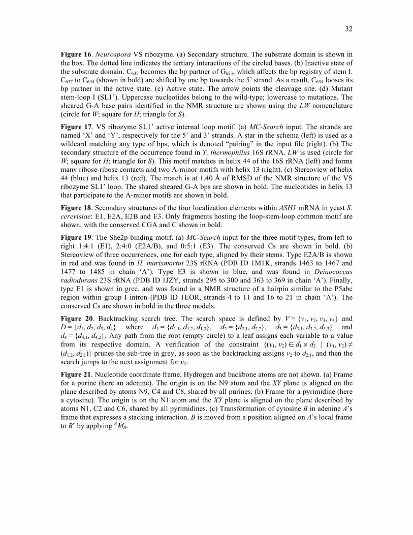
32

Figure 16. Neurospora VS ribozyme. (a) Secondary structure. The substrate domain is shown in the box. The dotted line indicates the tertiary interactions of the circled bases. (b) Inactive state of the substrate domain. C637 becomes the bp partner of G623, which affects the bp registry of stem I. C637 to C634 (shown in bold) are shifted by one bp towards the 5’ strand. As a result, C634 looses its bp partner in the active state. (c) Active state. The arrow points the cleavage site. (d) Mutant stem-loop I (SL1’). Uppercase nucleotides belong to the wild-type; lowercase to mutations. The sheared G-A base pairs identified in the NMR structure are shown using the LW nomenclature (circle for W; square for H; triangle for S).

Figure 17. VS ribozyme SL1’ active internal loop motif. (a) MC-Search input. The strands are named ‘X’ and ‘Y’, respectively for the 5’ and 3’ strands. A star in the schema (left) is used as a wildcard matching any type of bps, which is denoted “pairing” in the input file (right). (b) The secondary structure of the occurrence found in T. thermophilus 16S rRNA. LW is used (circle for W; square for H; triangle for S). This motif matches in helix 44 of the 16S rRNA (left) and forms many ribose-ribose contacts and two A-minor motifs with helix 13 (right). (c) Stereoview of helix 44 (blue) and helix 13 (red). The match is at 1.40 Å of RMSD of the NMR structure of the VS ribozyme SL1’ loop. The shared sheared G-A bps are shown in bold. The nucleotides in helix 13 that participate to the A-minor motifs are shown in bold.

Figure 18. Secondary structures of the four localization elements within ASH1 mRNA in yeast S. cerevisiae: E1, E2A, E2B and E3. Only fragments hosting the loop-stem-loop common motif are shown, with the conserved CGA and C shown in bold.

Figure 19. The She2p-binding motif. (a) MC-Search input for the three motif types, from left to right 1:4:1 (E1), 2:4:0 (E2A/B), and 0:5:1 (E3). The conserved Cs are shown in bold. (b) Stereoview of three occurrences, one for each type, aligned by their stems. Type E2A/B is shown in red and was found in H. marismortui 23S rRNA (PDB ID 1M1K, strands 1463 to 1467 and 1477 to 1485 in chain ‘A’). Type E3 is shown in blue, and was found in Deinococcus radiodurans 23S rRNA (PDB ID 1JZY, strands 295 to 300 and 363 to 369 in chain ‘A’). Finally, type E1 is shown in gree, and was found in a NMR structure of a hairpin similar to the P5abc region within group I intron (PDB ID 1EOR, strands 4 to 11 and 16 to 21 in chain ‘A’). The conserved Cs are shown in bold in the three models.

Figure 20. Backtracking search tree. The search space is defined by V = {v1, v2, v3, v4} and D = {d1, d2, d3, d4} where d1 = {d1,1, d1,2, d1,3}, d2 = {d2,1, d2,2}, d3 = {d3,1, d3,2, d3,3} and d4 = {d4,1, d4,2}. Any path from the root (empty circle) to a leaf assigns each variable to a value from its respective domain. A verification of the constraint {(v1, v2) ∈ d1 × d2 | (v1, v2) ≠ (d1,2, d2,1)} prunes the sub-tree in grey, as soon as the backtracking assigns v2 to d2,1, and then the search jumps to the next assignment for v2.

Figure 21. Nucleotide coordinate frame. Hydrogen and backbone atoms are not shown. (a) Frame for a purine (here an adenine). The origin is on the N9 atom and the XY plane is aligned on the plane described by atoms N9, C4 and C8, shared by all purines. (b) Frame for a pyrimidine (here a cytosine). The origin is on the N1 atom and the XY plane is aligned on the plane described by atoms N1, C2 and C6, shared by all pyrimidines. (c) Transformation of cytosine B in adenine A’s frame that expresses a stacking interaction. B is moved from a position aligned on A’s local frame to B’ by applying AMB.

33

Figure 22. A two stacked G=C bps CSP. (a) RNA graph. The vertices are in uppercase; arcs in lowercase. The arcs of a chosen spanning tree are shown in bold; rooted at vertex A (shaded). (b) One solution: the nucleotide structure for each vertex and a local transformation matrix for each arc (Mi for arc ‘i’). The root is aligned to the global coordinate frame O. B is positioned by applying Ma = AMB in the local frame A, which is aligned with O, and thus B is directly placed in the global frame by Ma; vertex C directly placed by Mb = AMC. Finally, to position D, Mc = CMD is applied in the local frame of C, which is then moved to the global frame by applying Mb = AMC. The O3’-P bond lengths shown in dashed lines are verified by a distance constraint. In this spanning tree, arc d is not considered in the construction.

Figure 23. Ribose construction. (a) A base and two phosphate groups. (b) The ribose structure is appended to the base and is parameterized by ρ and χ. The length of the implicit interconnections (shown in dashed lines), l5’ and l3’, respectively represent the covalent C5’-O5’ and C3’-O3’ bonds, which quantifies the precision of the construction.

Figure 24. Tandem W/W bps. (a) RNA graph. (b) Spanning tree. (c) MC-Sym input. The “stack” keyword is used as a wildcard matching any of the four stacking types: upward, downward, inward or outward.

Figure 25. Extraction of the A14-U8 H/W bp transformation in the yeast tRNA-Phe X-ray crystal structure (PDB ID 1EVV). A thread follows the strands by the phosphorus atoms. Hydrogen atoms are not shown. The bp is zoomed and shown with the frames (OMA14 and OMU8) defined in the global frame, O. The transformation A14MU8 = OMA14

-1 × OMU8 is extracted.

Figure 26. Yeast tRNA T-stem-loop. (a) Secondary structure. (b) MC-Sym input for the stem fragment. (c) MC-Sym input for the loop fragment. (d) MC-Sym input for merging both fragments. (e) Spanning tree of (b). (f) Spanning tree of (c). (g) Spanning tree of (d). (h) Stereoview of a final model generated by MC-Sym. The bases are shown in blue; the U54-A58 W/H bp in lighter blue. The backbone is shown in yellow. The thread follows the phosphodiester chain. Hydrogen atoms are not shown.