Embed Size (px)
Citation preview
User’s Guide for MapMark4—An R Package for the Probability Calculations in Three-Part Mineral Resource Assessments
Chapter 14 ofSection C, Computer ProgramsBook 7, Automated Data Processing and Computations
Techniques and Methods 7–C14
U.S. Department of the InteriorU.S. Geological Survey

User’s Guide for MapMark4— An R Package for the Probability Calculations in Three-Part Mineral Resource Assessments
By Karl J. Ellefsen
Chapter 14 ofSection C, Computer ProgramsBook 7, Automated Data Processing and Computations
Techniques and Methods 7–C14
U.S. Department of the InteriorU.S. Geological Survey

U.S. Department of the InteriorRYAN K. ZINKE, Secretary
U.S. Geological SurveyWilliam H. Werkheiser, Acting Director
U.S. Geological Survey, Reston, Virginia: 2017
For more information on the USGS—the Federal source for science about the Earth, its natural and living resources, natural hazards, and the environment—visit https://www.usgs.gov or call 1–888–ASK–USGS.
For an overview of USGS information products, including maps, imagery, and publications, visit https://store.usgs.gov.
Any use of trade, firm, or product names is for descriptive purposes only and does not imply endorsement by the U.S. Government.
Although this information product, for the most part, is in the public domain, it also may contain copyrighted materials as noted in the text. Permission to reproduce copyrighted items must be secured from the copyright owner.
Suggested citation:Ellefsen, K.J., 2017, User’s guide for MapMark4—An R package for the probability calculations in three-part mineral resource assessments: U.S. Geological Survey Techniques and Methods, book 7, chap. C14, 23 p., https://doi.org/10.3133/tm7C14.
ISSN 2328-7055 (online)
iii
Contents
Abstract ...........................................................................................................................................................1Introduction.....................................................................................................................................................1Overview of Probability Calculations .........................................................................................................1Data for Probability Calculations ................................................................................................................2
Grade and Tonnage Model ..................................................................................................................2Estimates of the Number of Undiscovered Deposits ......................................................................3
Preparatory Steps ..........................................................................................................................................4Probability Calculations ................................................................................................................................4
Metadata ................................................................................................................................................4Distribution for the Ore Tonnages ......................................................................................................5Distribution for the Grades ..................................................................................................................7Distribution for the Number of Undiscovered Deposits ...............................................................11Simulation.............................................................................................................................................12Distribution for the Total Ore and Mineral Resource Tonnages in all Simulated
Undiscovered Deposits ........................................................................................................12Archive of the Calculation Results ............................................................................................................16Acknowledgments .......................................................................................................................................17References Cited..........................................................................................................................................17Appendix 1. Probability Calculations for a Tonnage Model ..............................................................19
Overview...............................................................................................................................................19Data .......................................................................................................................................................19Preparatory Steps, Probability Calculations, and Archive of the Results .................................19
Appendix 2. Custom Distribution for the Number of Undiscovered Deposits ................................21Appendix 3. Installation Instructions ....................................................................................................23
Required Packages.............................................................................................................................23Installation Instructions for MapMark4 When Using RStudio ....................................................23Installation Instructions for MapMark4 When Using RGui ..........................................................23
Appendix 4. Calculation Scripts .............................................................................................................23
Figures
1. Diagram showing general relations among the inputs to the probability calculations, the six software classes, and the output ........................................................................................2
2. A, Graphs showing probability density function that represents the ore tonnage in an undiscovered deposit. B, Corresponding cumulative distribution function ..............6
3. Histograms (A, B, and C) and cumulative distribution functions (D, E, and F ) that are calculated from the probability density function representing the grades .................8
4–6. Graphs showing: 4. A, Negative binomial probability mass function representing the number of
undiscovered deposits in the permissive tract. B, Probability mass function recast as elicitation percentiles and compared to the estimated numbers of undiscovered deposits ...................................................................................................11
iv
5. A, Univariate, marginal, probability density functions and B, univariate, marginal, complementary cumulative distribution functions for the total ore and mineral resource tonnages in all undiscovered deposits within the permissive tract .................. 13
6. A–I, Univariate and bivariate marginal distributions for the ore and mineral resource tonnages in all undiscovered deposits within the permissive tract ..........14
Appendix Figures
1–1. Diagram showing general relations among the inputs to the probability calculations, the five software classes, and the output ......................................................................................... 19
2–1. Graph showing example of a custom pmf for the number of undiscovered deposits in the permissive tract ............................................................................................................................ 21
Conversion Factors
International System of Units to Inch/Pound
Multiply By To obtainMass
kilogram (kg) 2.205 pound avoirdupois (lb)
User’s Guide for MapMark4—An R Package for the Probability Calculations in Three-Part Mineral Resource Assessments
By Karl J. Ellefsen
Abstract
MapMark4 is a software package that implements the probability calculations in three-part mineral resource assessments. Functions within the software package are written in the R statistical programming language. These functions, their documenta-tion, and a copy of this user’s guide are bundled together in R’s unit of shareable code, which is called a “package.” This user’s guide includes step-by-step instructions showing how the functions are used to carry out the probability calculations. The calcu-lations are demonstrated using test data, which are included in the package.
Introduction
MapMark4 is a software package that implements the probability calculations in three-part mineral resource assessments. The name is derived from the descriptive phrase “mineral assessment program mark4”—the name “mark4” is chosen because the previ-ous, similar program was called “mark3” (Root and others, 1992). Functions within the software package are written in the R statis-tical programming language, which is called either “R language” or “R” in this user’s guide. These functions, their documentation, and a copy of this user’s guide are bundled together in R’s unit of sharable code, which is called a “package.” MapMark4 provides the essential R functions to perform the probability calculations but does not provide a graphical user’s interface.
This user’s guide provides an overview of the MapMark4 package, showing you how to use the functions to carry out the probability calculations. As an overview, the scope of this user’s guide is limited. It does not provide detailed descriptions of the functions because this information is available in the package Help. It describes neither the underlying probability model nor the mathematics of the calculations, because this information is published in Ellefsen (2017).
We assume that you are familiar with the R language, statistical methods, compositional data analysis, and the method of three-part mineral resource assessment. That is, we assume that you are an advanced user. Furthermore, we assume that you are using the Windows operating system. If not, then you must modify those steps in the user’s guide that are related to files and directories.
The goals of this user’s guide are most readily achieved by showing the step-by-step calculations for an actual dataset. Thus, the package includes two datasets for your use. This user’s guide includes the R-language scripts that carry out the step-by-step calculations on these datasets. We strongly encourage you to execute these scripts yourself because this effort will help you become familiar with the calculations.
This user’s guide focuses primarily on probability calculations involving grade and tonnage models, which specify ore ton-nage and mineral resource grades. However, probability calculations also can be performed for tonnage models, which specify contained metal tonnage. These calculations are described in Appendix 1.
In this user’s guide, R language scripts, program variables, data structures, and so on are typeset using the Courier New font (for example, setwd(“F:\\tmp\\PT001”)).
Overview of Probability Calculations
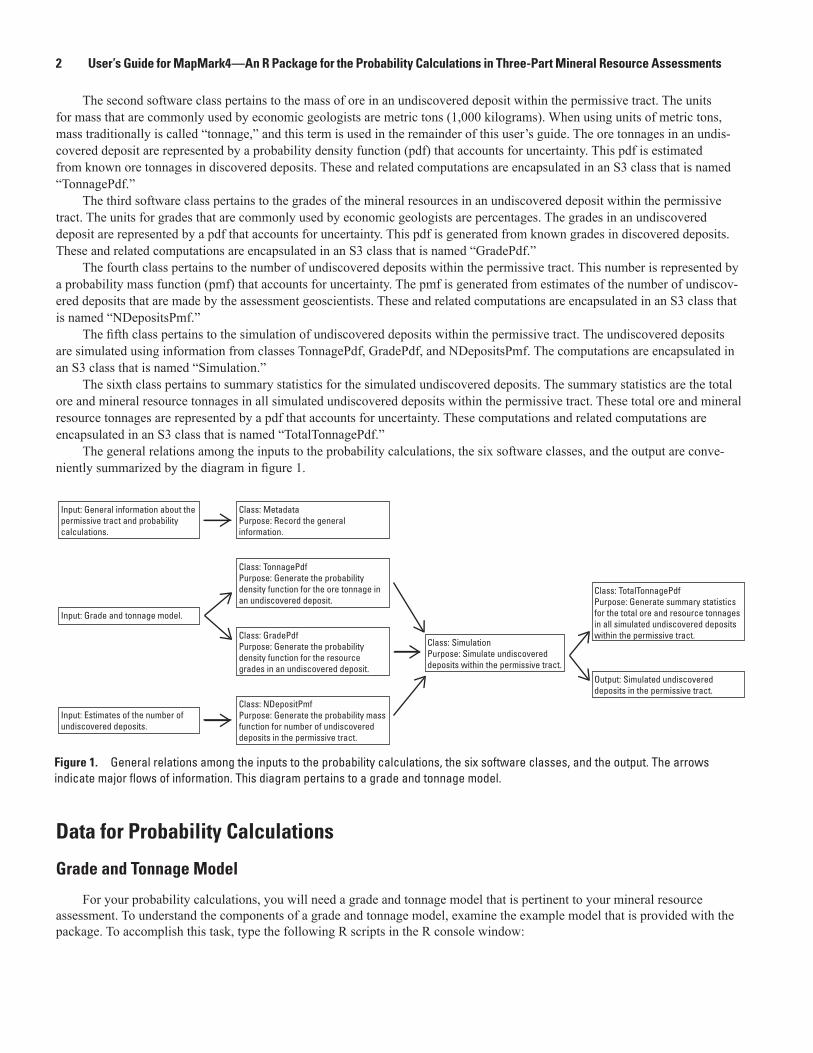
The probability calculations are conveniently divided into six groups, which are implemented as software classes. The first class pertains to the metadata that describes the permissive tract. The metadata are encapsulated in an S3 class, which is one type of an R language class (R Core Team, 2015). This class is named “Metadata.”
2 User’s Guide for MapMark4—An R Package for the Probability Calculations in Three-Part Mineral Resource Assessments
The second software class pertains to the mass of ore in an undiscovered deposit within the permissive tract. The units for mass that are commonly used by economic geologists are metric tons (1,000 kilograms). When using units of metric tons, mass traditionally is called “tonnage,” and this term is used in the remainder of this user’s guide. The ore tonnages in an undis-covered deposit are represented by a probability density function (pdf) that accounts for uncertainty. This pdf is estimated from known ore tonnages in discovered deposits. These and related computations are encapsulated in an S3 class that is named “TonnagePdf.”
The third software class pertains to the grades of the mineral resources in an undiscovered deposit within the permissive tract. The units for grades that are commonly used by economic geologists are percentages. The grades in an undiscovered deposit are represented by a pdf that accounts for uncertainty. This pdf is generated from known grades in discovered deposits. These and related computations are encapsulated in an S3 class that is named “GradePdf.”
The fourth class pertains to the number of undiscovered deposits within the permissive tract. This number is represented by a probability mass function (pmf) that accounts for uncertainty. The pmf is generated from estimates of the number of undiscov-ered deposits that are made by the assessment geoscientists. These and related computations are encapsulated in an S3 class that is named “NDepositsPmf.”
The fifth class pertains to the simulation of undiscovered deposits within the permissive tract. The undiscovered deposits are simulated using information from classes TonnagePdf, GradePdf, and NDepositsPmf. The computations are encapsulated in an S3 class that is named “Simulation.”
The sixth class pertains to summary statistics for the simulated undiscovered deposits. The summary statistics are the total ore and mineral resource tonnages in all simulated undiscovered deposits within the permissive tract. These total ore and mineral resource tonnages are represented by a pdf that accounts for uncertainty. These computations and related computations are encapsulated in an S3 class that is named “TotalTonnagePdf.”
The general relations among the inputs to the probability calculations, the six software classes, and the output are conve-niently summarized by the diagram in figure 1.
Data for Probability Calculations
Grade and Tonnage Model
For your probability calculations, you will need a grade and tonnage model that is pertinent to your mineral resource assessment. To understand the components of a grade and tonnage model, examine the example model that is provided with the package. To accomplish this task, type the following R scripts in the R console window:
Input: General information about thepermissive tract and probability calculations.
Class: MetadataPurpose: Record the generalinformation.
Class: SimulationPurpose: Simulate undiscovereddeposits within the permissive tract.
Class: TonnagePdfPurpose: Generate the probabilitydensity function for the ore tonnage inan undiscovered deposit.
Class: TotalTonnagePdfPurpose: Generate summary statisticsfor the total ore and resource tonnagesin all simulated undiscovered depositswithin the permissive tract.Class: GradePdf
Purpose: Generate the probabilitydensity function for the resourcegrades in an undiscovered deposit.
Class: NDepositPmfPurpose: Generate the probability massfunction for number of undiscovereddeposits in the permissive tract.
Input: Estimates of the number ofundiscovered deposits.
Output: Simulated undiscovereddeposits in the permissive tract.
Input: Grade and tonnage model.
Figure 1. General relations among the inputs to the probability calculations, the six software classes, and the output. The arrows indicate major flows of information. This diagram pertains to a grade and tonnage model.
Data for Probability Calculations 3
library(MapMark4)
ExampleGatm
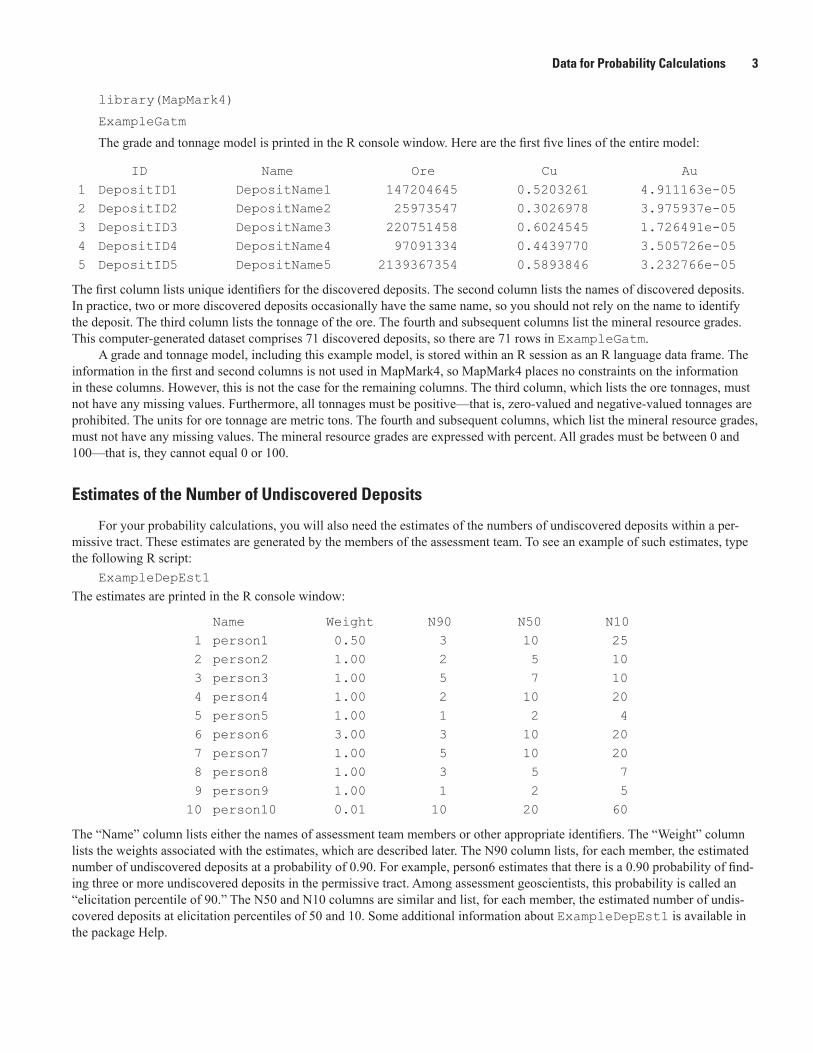
The grade and tonnage model is printed in the R console window. Here are the first five lines of the entire model:
ID Name Ore Cu Au1 DepositID1 DepositName1 147204645 0.5203261 4.911163e-052 DepositID2 DepositName2 25973547 0.3026978 3.975937e-053 DepositID3 DepositName3 220751458 0.6024545 1.726491e-054 DepositID4 DepositName4 97091334 0.4439770 3.505726e-055 DepositID5 DepositName5 2139367354 0.5893846 3.232766e-05
The first column lists unique identifiers for the discovered deposits. The second column lists the names of discovered deposits. In practice, two or more discovered deposits occasionally have the same name, so you should not rely on the name to identify the deposit. The third column lists the tonnage of the ore. The fourth and subsequent columns list the mineral resource grades. This computer-generated dataset comprises 71 discovered deposits, so there are 71 rows in ExampleGatm.
A grade and tonnage model, including this example model, is stored within an R session as an R language data frame. The information in the first and second columns is not used in MapMark4, so MapMark4 places no constraints on the information in these columns. However, this is not the case for the remaining columns. The third column, which lists the ore tonnages, must not have any missing values. Furthermore, all tonnages must be positive—that is, zero-valued and negative-valued tonnages are prohibited. The units for ore tonnage are metric tons. The fourth and subsequent columns, which list the mineral resource grades, must not have any missing values. The mineral resource grades are expressed with percent. All grades must be between 0 and 100—that is, they cannot equal 0 or 100.
Estimates of the Number of Undiscovered Deposits
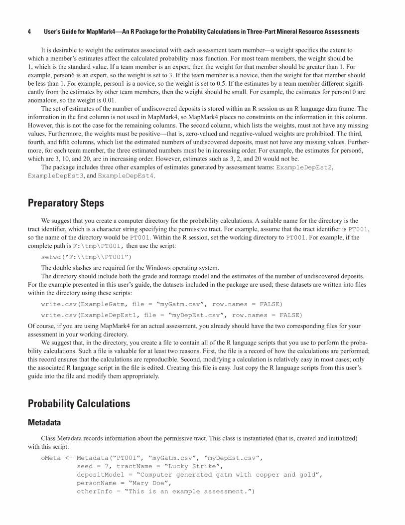
For your probability calculations, you will also need the estimates of the numbers of undiscovered deposits within a per-missive tract. These estimates are generated by the members of the assessment team. To see an example of such estimates, type the following R script:
ExampleDepEst1
The estimates are printed in the R console window:
Name Weight N90 N50 N101 person1 0.50 3 10 252 person2 1.00 2 5 103 person3 1.00 5 7 104 person4 1.00 2 10 205 person5 1.00 1 2 46 person6 3.00 3 10 207 person7 1.00 5 10 208 person8 1.00 3 5 79 person9 1.00 1 2 5
10 person10 0.01 10 20 60
The “Name” column lists either the names of assessment team members or other appropriate identifiers. The “Weight” column lists the weights associated with the estimates, which are described later. The N90 column lists, for each member, the estimated number of undiscovered deposits at a probability of 0.90. For example, person6 estimates that there is a 0.90 probability of find-ing three or more undiscovered deposits in the permissive tract. Among assessment geoscientists, this probability is called an “elicitation percentile of 90.” The N50 and N10 columns are similar and list, for each member, the estimated number of undis-covered deposits at elicitation percentiles of 50 and 10. Some additional information about ExampleDepEst1 is available in the package Help.
4 User’s Guide for MapMark4—An R Package for the Probability Calculations in Three-Part Mineral Resource Assessments
It is desirable to weight the estimates associated with each assessment team member—a weight specifies the extent to which a member’s estimates affect the calculated probability mass function. For most team members, the weight should be 1, which is the standard value. If a team member is an expert, then the weight for that member should be greater than 1. For example, person6 is an expert, so the weight is set to 3. If the team member is a novice, then the weight for that member should be less than 1. For example, person1 is a novice, so the weight is set to 0.5. If the estimates by a team member different signifi-cantly from the estimates by other team members, then the weight should be small. For example, the estimates for person10 are anomalous, so the weight is 0.01.
The set of estimates of the number of undiscovered deposits is stored within an R session as an R language data frame. The information in the first column is not used in MapMark4, so MapMark4 places no constraints on the information in this column. However, this is not the case for the remaining columns. The second column, which lists the weights, must not have any missing values. Furthermore, the weights must be positive—that is, zero-valued and negative-valued weights are prohibited. The third, fourth, and fifth columns, which list the estimated numbers of undiscovered deposits, must not have any missing values. Further-more, for each team member, the three estimated numbers must be in increasing order. For example, the estimates for person6, which are 3, 10, and 20, are in increasing order. However, estimates such as 3, 2, and 20 would not be.
The package includes three other examples of estimates generated by assessment teams: ExampleDepEst2, ExampleDepEst3, and ExampleDepEst4.
Preparatory Steps
We suggest that you create a computer directory for the probability calculations. A suitable name for the directory is the tract identifier, which is a character string specifying the permissive tract. For example, assume that the tract identifier is PT001, so the name of the directory would be PT001. Within the R session, set the working directory to PT001. For example, if the complete path is F:\tmp\PT001, then use the script:
setwd(“F:\\tmp\\PT001”)
The double slashes are required for the Windows operating system.The directory should include both the grade and tonnage model and the estimates of the number of undiscovered deposits.
For the example presented in this user’s guide, the datasets included in the package are used; these datasets are written into files within the directory using these scripts:
write.csv(ExampleGatm, file = “myGatm.csv”, row.names = FALSE)
write.csv(ExampleDepEst1, file = “myDepEst.csv”, row.names = FALSE)
Of course, if you are using MapMark4 for an actual assessment, you already should have the two corresponding files for your assessment in your working directory.
We suggest that, in the directory, you create a file to contain all of the R language scripts that you use to perform the proba-bility calculations. Such a file is valuable for at least two reasons. First, the file is a record of how the calculations are performed; this record ensures that the calculations are reproducible. Second, modifying a calculation is relatively easy in most cases; only the associated R language script in the file is edited. Creating this file is easy. Just copy the R language scripts from this user’s guide into the file and modify them appropriately.
Probability Calculations
Metadata
Class Metadata records information about the permissive tract. This class is instantiated (that is, created and initialized) with this script:
oMeta <- Metadata(“PT001”, “myGatm.csv”, “myDepEst.csv”, seed = 7, tractName = “Lucky Strike”, depositModel = “Computer generated gatm with copper and gold”, personName = “Mary Doe”, otherInfo = “This is an example assessment.”)
Probability Calculations 5
The first argument is the tract identifier, which is a character string that uniquely identifies the tract. The tract identifier is used to generate file names for which the associated files record information about the probability calculations. Consequently, it is important to pick a tract identifier that is also suitable for file names—it should not contain nonstandard characters. The second argument is the name of the file containing the grade and tonnage model. The third argument is the name of the file containing the estimates of the number of undiscovered deposits that were made by the assessment team. The remaining arguments are optional. Argument seed, which is a positive integer, is used to set the state of the random number generator. If seed is speci-fied, then probability calculations will always yield the same results—the probability calculations will be exactly reproducible. Argument tractName is the name of the tract. Argument depositModel is the name of the descriptive model used for the mineral resource that is being assessed (Singer and Menzie, 2010, p. 29–41). Argument personName is the name of the person performing the probability calculations. Argument otherInfo contains additional information regarding the probability calcu-lations and the assessment itself.
This scriptsummary(oMeta)
prints the following summary to the R console:Metadata for the permissive tract-----------------------------------------------------------------------------------Tract identifier: PT001Name of file containing the model: myGatm.csvName of file containing the estimates of the number of deposits: myDepEst.csvSeed: 7Tract name: Lucky StrikeDeposit model: Computer generated gatm with copper and goldCalculation date: Fri Dec 09 11:13:08 2016Name of person performing the calculations: Mary DoeOther information: This is an example assessment.
##################################################################################
Notice that the summary includes an additional field Calculation date, which is the date and time that the probability calculations are performed. This field can be set manually using an argument to function MetaData—see the package Help for details.
Distribution for the Ore Tonnages
Class TonnagePdf generates the pdf that represents the ore tonnages in an undiscovered deposit within the permissive tract. The pdf is estimated from the grade and tonnage model, which is described in section “Data for probability calculations.” The grade and tonnage model is read with this script:
gatm <- read.csv(getModelFilename(oMeta))
Function getModelFilename gets the name of the file containing the grade and tonnage model from the metadata, and then function read.csv reads that file. Then class TonnagePdf is instantiated with this script:
oTonPdf <- TonnagePdf(gatm, seed = getSeed(oMeta))
The first argument is the R-language data frame containing the grade and tonnage model. The second argument seed is set to the value that is stored in the metadata, which is obtained with function getSeed. There are two additional, optional arguments to function TonnagePdf that are particularly important. Argument pdfType specifies the type of pdf. The default type is normal, which is a normal pdf. The other available type is kde, which is a kernel density estimate. Argument isTruncated specifies whether the pdf is truncated at the lowest and highest ore tonnages in the grade and tonnage model. The default value is FALSE, and the other value is TRUE.
When there are less than roughly 50 discovered deposits in the grade and tonnage model, there are, of course, few ore ton-nages with which to estimate the pdf. In such cases, we suggest that you use the normal pdf. Conversely, when there are more than roughly 50 discovered deposits in the grade and tonnage model, you might consider using the kernel density estimate pdf. These guidelines are not rules, so you should check the pdfs generated with both methods.
A simple way to check the pdf is to plot both it and its cumulative distribution function (cdf):plot(oTonPdf)
6 User’s Guide for MapMark4—An R Package for the Probability Calculations in Three-Part Mineral Resource Assessments
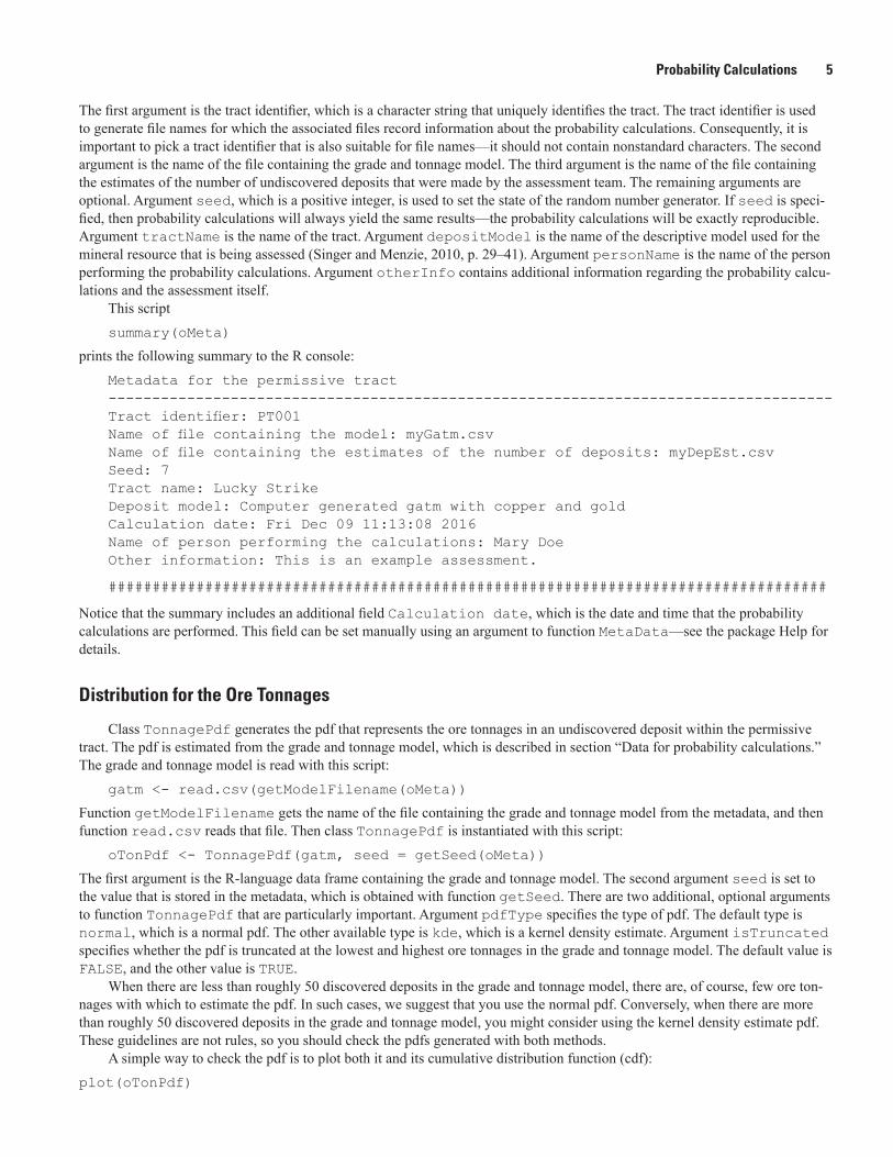
The resulting plot is shown in figure 2. Notice that both horizontal axes are logarithmic because the range of the ore tonnage is enormous. In fig. 2A, the pdf, which is represented by the histogram, spans the range of the ore tonnages from the grade and tonnage model. Furthermore, the pdf is large exactly where the density of ore tonnages is high (that is, roughly 3×10⁷ to 1×10⁹ metric tons). In fig. 2B, the cdf matches the empirical cdf. Thus, we conclude that the pdf adequately represents the ore tonnages in the grade and tonnage model.
Deviance (fig. 2B) is a statistic that quantifies the misfit between the ore tonnages from the discovered deposits and the pdf that represents those ore tonnages. Small values indicate a better fit than large values do. This information can help you decide which type of pdf is best suited for your data.
0
0.2
0.4
0.6 1.00
0.75
0.50
0.25
01e+07 1e+071e+09 1e+09
Dens
ity
A B
Deviance = –26
Ore tonnage, in metric tons Ore tonnage, in metric tons
Prob
abili
ty
DEN0041_fig_02\\IGSKAHCMVSFS002\Pubs_Common\Jeff\den17_cmrp00_0041_tm_ellefson\report_figures
Figure 2. A, Probability density function that represents the ore tonnage in an undiscovered deposit. The vertical lines at the bottom represent the ore tonnages from the grade and tonnage model. B, Corresponding cumulative distribution function (solid line). The red dots constitute the empirical cumulative distribution function for the ore tonnages from the grade and tonnage model.
This script
summary(oTonPdf)
prints the following summary to the R console:
Summary comparison of the pdf representing the tonnage and the actual tonnages in the model.
--------------------------------------------------------------------------------------
Pdf type: normal
Pdf is not truncated.
Number of discovered deposits in the model: 71
Deviance = -26.0251
--------------------------------------------------------------------------------------
This table pertains to the log-transformed tonnages.
Column Gatm refers to the actual tonnages in the
grade and tonnage model; column Pdf refers to the pdf
representing the tonnages.
Gatm Pdf
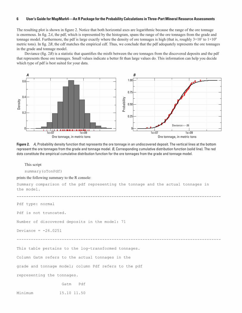
Minimum 15.10 11.50
Probability Calculations 7
0.25 quantile 18.00 18.00
Median 19.00 19.00
0.75 quantile 20.30 20.10
Maximum 22.20 26.20
Mean 19.00 19.00
Standard deviation 1.49 1.49
--------------------------------------------------------------------------------------
This table pertains to the (untransformed) tonnages.
Column Gatm refers to the tonnages in the grade and
tonnage model; column Pdf refers to the pdf representing the tonnages.
Gatm Pdf
Minimum 3.70e+06 9.73e+04
0.25 quantile 6.64e+07 6.85e+07
Median 1.72e+08 1.87e+08
0.75 quantile 6.26e+08 5.13e+08
Maximum 4.39e+09 2.35e+11
Mean 4.67e+08 5.68e+08
Standard deviation 6.89e+08 1.61e+09
######################################################################################
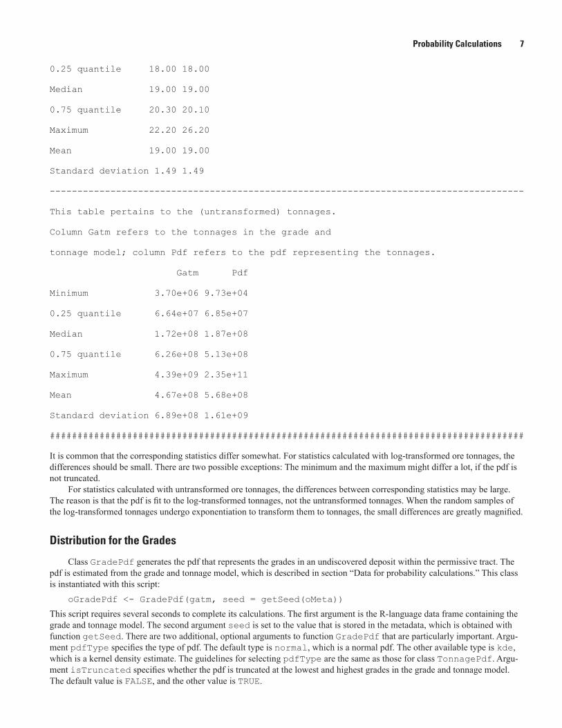
It is common that the corresponding statistics differ somewhat. For statistics calculated with log-transformed ore tonnages, the differences should be small. There are two possible exceptions: The minimum and the maximum might differ a lot, if the pdf is not truncated.
For statistics calculated with untransformed ore tonnages, the differences between corresponding statistics may be large. The reason is that the pdf is fit to the log-transformed tonnages, not the untransformed tonnages. When the random samples of the log-transformed tonnages undergo exponentiation to transform them to tonnages, the small differences are greatly magnified.
Distribution for the Grades
Class GradePdf generates the pdf that represents the grades in an undiscovered deposit within the permissive tract. The pdf is estimated from the grade and tonnage model, which is described in section “Data for probability calculations.” This class is instantiated with this script:
oGradePdf <- GradePdf(gatm, seed = getSeed(oMeta))
This script requires several seconds to complete its calculations. The first argument is the R-language data frame containing the grade and tonnage model. The second argument seed is set to the value that is stored in the metadata, which is obtained with function getSeed. There are two additional, optional arguments to function GradePdf that are particularly important. Argu-ment pdfType specifies the type of pdf. The default type is normal, which is a normal pdf. The other available type is kde, which is a kernel density estimate. The guidelines for selecting pdfType are the same as those for class TonnagePdf. Argu-ment isTruncated specifies whether the pdf is truncated at the lowest and highest grades in the grade and tonnage model. The default value is FALSE, and the other value is TRUE.
8 User’s Guide for MapMark4—An R Package for the Probability Calculations in Three-Part Mineral Resource Assessments
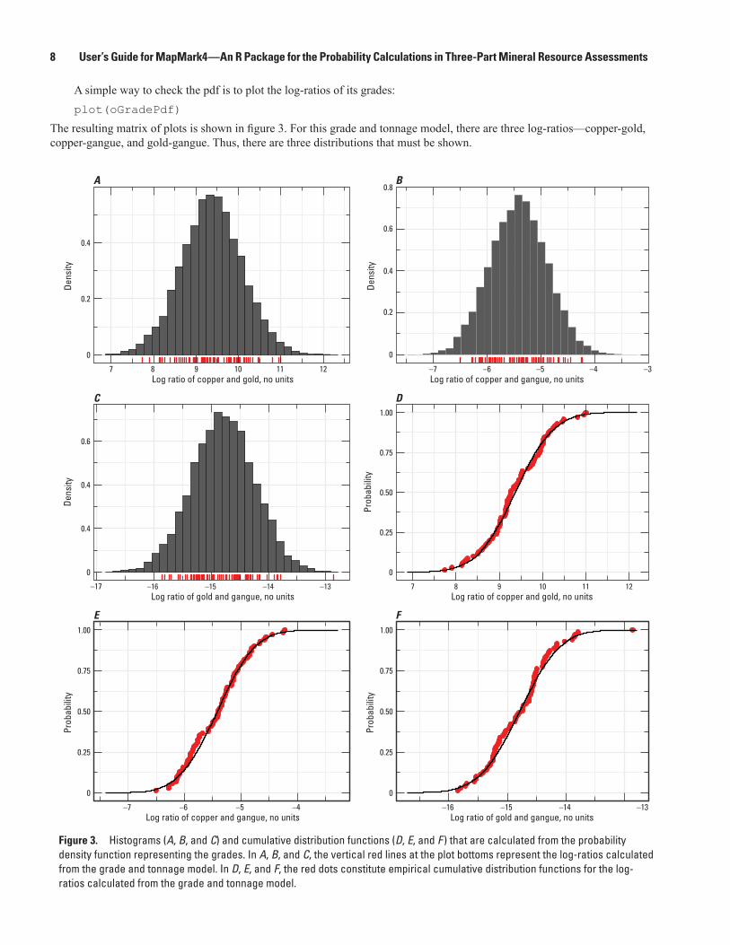
A simple way to check the pdf is to plot the log-ratios of its grades:plot(oGradePdf)
The resulting matrix of plots is shown in figure 3. For this grade and tonnage model, there are three log-ratios—copper-gold, copper-gangue, and gold-gangue. Thus, there are three distributions that must be shown.
0.4
0.6
0.4
0.4
0
0.6
0.4
0.2
0
0.8
0.2
0
7 8 10 11 12 –7 –6 –5 –4 –39
Dens
ityDe
nsity
0.50
0.25
0
0.75
1.00
Prob
abili
ty
0.50
0.25
0
0.75
1.00
Prob
abili
ty
0.50
0.25
0
0.75
1.00
Prob
abili
tyDe
nsity
Log ratio of copper and gold, no units
–17 –16 –15 –14 –13Log ratio of gold and gangue, no units
–7 –6 –5 –4Log ratio of copper and gangue, no units
–16 –15 –14 –13Log ratio of gold and gangue, no units
7 8 9 10 11 12Log ratio of copper and gold, no units
Log ratio of copper and gangue, no units
A B
C D
E F
Figure 3. Histograms (A, B, and C) and cumulative distribution functions (D, E, and F ) that are calculated from the probability density function representing the grades. In A, B, and C, the vertical red lines at the plot bottoms represent the log-ratios calculated from the grade and tonnage model. In D, E, and F, the red dots constitute empirical cumulative distribution functions for the log-ratios calculated from the grade and tonnage model.
Probability Calculations 9
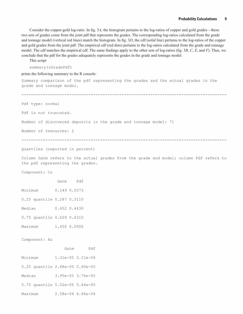
Consider the copper-gold log-ratio. In fig. 3A, the histogram pertains to the log-ratios of copper and gold grades—these two sets of grades come from the joint pdf that represents the grades. The corresponding log-ratios calculated from the grade and tonnage model (vertical red lines) match the histogram. In fig. 3D, the cdf (solid line) pertains to the log-ratios of the copper and gold grades from the joint pdf. The empirical cdf (red dots) pertains to the log-ratios calculated from the grade and tonnage model. The cdf matches the empirical cdf. The same findings apply to the other sets of log-ratios (fig. 3B, C, E, and F). Thus, we conclude that the pdf for the grades adequately represents the grades in the grade and tonnage model.
This script
summary(oGradePdf)
prints the following summary to the R console:
Summary comparison of the pdf representing the grades and the actual grades in the grade and tonnage model.
--------------------------------------------------------------------------------------
Pdf type: normal
Pdf is not truncated.
Number of discovered deposits in the grade and tonnage model: 71
Number of resources: 2
--------------------------------------------------------------------------------------
Quantiles (reported in percent)
Column Gatm refers to the actual grades from the grade and model; column Pdf refers to the pdf representing the grades.
Component: Cu
Gatm Pdf
Minimum 0.149 0.0373
0.25 quantile 0.287 0.3110
Median 0.452 0.4430
0.75 quantile 0.629 0.6310
Maximum 1.450 6.0900
Component: Au
Gatm Pdf
Minimum 1.31e-05 2.11e-06
0.25 quantile 2.48e-05 2.60e-05
Median 3.95e-05 3.76e-05
0.75 quantile 5.02e-05 5.44e-05
Maximum 2.58e-04 6.46e-04
10 User’s Guide for MapMark4—An R Package for the Probability Calculations in Three-Part Mineral Resource Assessments
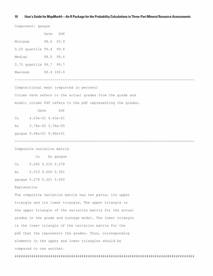
Component: gangue
Gatm Pdf
Minimum 98.6 93.9
0.25 quantile 99.4 99.4
Median 99.5 99.6
0.75 quantile 99.7 99.7
Maximum 99.9 100.0
--------------------------------------------------------------------------------------
Compositional mean (reported in percent)
Column Gatm refers to the actual grades from the grade and
model; column Pdf refers to the pdf representing the grades.
Gatm Pdf
Cu 4.43e-01 4.43e-01
Au 3.76e-05 3.76e-05
gangue 9.96e+01 9.96e+01
--------------------------------------------------------------------------------------
Composite variation matrix
Cu Au gangue
Cu 0.000 0.510 0.278
Au 0.510 0.000 0.301
gangue 0.278 0.301 0.000
Explanation
The composite variation matrix has two parts: its upper
triangle and its lower triangle. The upper triangle is
the upper triangle of the variation matrix for the actual
grades in the grade and tonnage model. The lower triangle
is the lower triangle of the variation matrix for the
pdf that the represents the grades. Thus, corresponding
elements in the upper and lower triangles should be
compared to one another.
######################################################################################
Probability Calculations 11
Corresponding statistics usually differ slightly. However, if the pdf is not truncated, then the corresponding minimum and the maximum statistics might differ a lot, as they do in this example. (Some readers may notice that the maximum percentage for gangue is 100, which appears to contradict the criteria listed in section “Grade and tonnage model.” The actual value is slightly less than 100, but has been rounded to 100 for the summary.)
Distribution for the Number of Undiscovered Deposits
Class NDepositPmf generates the pmf for the number of undiscovered deposits in the permissive tract. This pmf is cal-culated from the estimates of the number of undiscovered deposits, which is described in section “Data for probability calcula-tions.” The estimates are read with this script:
depEst <- read.csv(getDepEstFilename(oMeta))
Function getDepEstFilename gets the name of the file containing the estimates from the metadata, and then function read.csv reads that file. Then class NDepositPmf is instantiated with this script:
oPmf <- NDepositsPmf(“NegBinomial”, list(nDepEst = depEst))The function requires several seconds to complete its calculations. The first argument specifies that the pmf is a negative bino-mial distribution. The second argument is an R-language list that comprises the parameters for the pmf. Parameter nDepEst is an R-language data frame that contains the estimates of the number of undiscovered deposits.
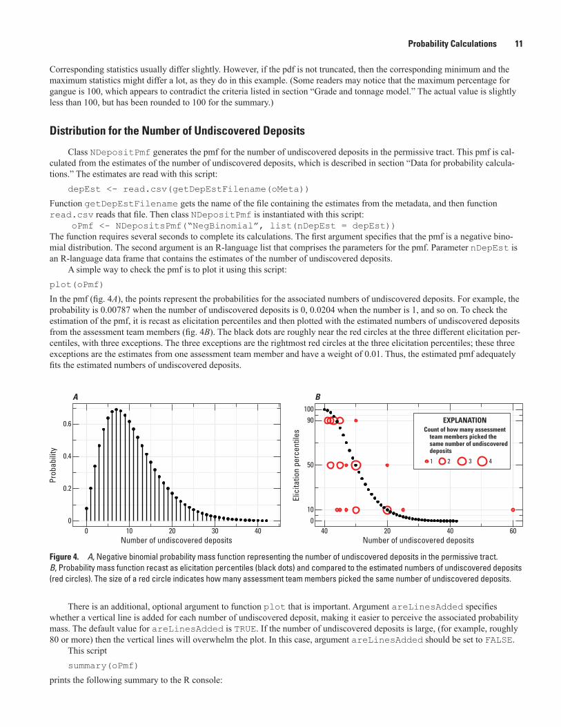
A simple way to check the pmf is to plot it using this script:plot(oPmf)
In the pmf (fig. 4A), the points represent the probabilities for the associated numbers of undiscovered deposits. For example, the probability is 0.00787 when the number of undiscovered deposits is 0, 0.0204 when the number is 1, and so on. To check the estimation of the pmf, it is recast as elicitation percentiles and then plotted with the estimated numbers of undiscovered deposits from the assessment team members (fig. 4B). The black dots are roughly near the red circles at the three different elicitation per-centiles, with three exceptions. The three exceptions are the rightmost red circles at the three elicitation percentiles; these three exceptions are the estimates from one assessment team member and have a weight of 0.01. Thus, the estimated pmf adequately fits the estimated numbers of undiscovered deposits.
DEN0041_fig_04\\IGSKAHCMVSFS002\Pubs_Common\Jeff \den17_cmrp00_0041_tm_ellefson\report_figures
There is an additional, optional argument to function plot that is important. Argument areLinesAdded specifies whether a vertical line is added for each number of undiscovered deposit, making it easier to perceive the associated probability mass. The default value for areLinesAdded is TRUE. If the number of undiscovered deposits is large, (for example, roughly 80 or more) then the vertical lines will overwhelm the plot. In this case, argument areLinesAdded should be set to FALSE.
This scriptsummary(oPmf)
prints the following summary to the R console:
0.6 90
50
100
100
0.2
0
0.4
0 10 20 30 40 40 20 40 60
Prob
abili
ty
Elic
itatio
n pe
rcen
tiles
A B
Number of undiscovered deposits Number of undiscovered deposits
Count of how many assessment team members picked the same number of undiscovered deposits
EXPLANATION
1 2 3 4
Figure 4. A, Negative binomial probability mass function representing the number of undiscovered deposits in the permissive tract. B, Probability mass function recast as elicitation percentiles (black dots) and compared to the estimated numbers of undiscovered deposits (red circles). The size of a red circle indicates how many assessment team members picked the same number of undiscovered deposits.
12 User’s Guide for MapMark4—An R Package for the Probability Calculations in Three-Part Mineral Resource Assessments
Summary of the pmf for the number of undiscovered deposits within the permissive tract.
--------------------------------------------------------------------------------------
Type: NegBinomial
Description:
Mean: 10.6613
Variance: 43.0923
Standard deviation: 6.56447
Mode: 7
Smallest number of deposits in the pmf: 0
Largest number of deposits in the pmf: 42
Information entropy: 3.19684
######################################################################################
Class NDepositPmf can generate one other type of pmf, which might be helpful in special situations; it is described in Appendix 2.
Simulation
Class Simulation, which simulates undiscovered deposits in the permissive tract, is instantiated with this script:
oSimulation <- Simulation(oPmf, oTonPdf, oGradePdf, seed = getSeed(oMeta))
The first argument is the object containing the pmf for the number of undiscovered deposits in the permissive tract, the second argument is the object containing the pdf for the ore tonnages in an undiscovered deposit, and the third argument is the object containing the pdf for the grades in an undiscovered deposit. The fourth argument seed is set to the value that is stored in the metadata, which is obtained with function getSeed.
Distribution for the Total Ore and Mineral Resource Tonnages in all Simulated Undiscovered Deposits
Assessment geoscientists usually desire a summary of the simulated mineral resource amounts. To this end, they use sum-mary statistics of total ore and mineral resource tonnages in all simulated undiscovered deposits within the permissive tract. These total tonnages are just the sum of the tonnages in the individual, simulated undiscovered deposits within the permissive tract. To calculate these statistics, it is necessary to calculate the distribution of the total ore and mineral resource tonnages. This distribution is calculated using class TotalTonnagePdf, which is instantiated with this script:
oTotalTonPdf <- TotalTonnagePdf(oSimulation, oPmf, oTonPdf, oGradePdf)
The first argument is an object of class DepositSim, the second of class NDepositsPmf, the third of class TonnagePdf, and the fourth of class GradePdf.
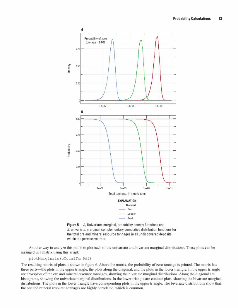
One way to analyze this pdf is to plot the univariate, marginal distributions of the total tonnages. This plot is generated with this script:
plot(oTotalTonPdf)
The univariate, marginal pdfs are shown in figure 5A. In the lower left corner of the plot, the probability of zero tonnage is printed. This probability will be nonzero whenever the pmf for the number of undiscovered deposits has a nonzero probability for zero deposits (fig. 4). The univariate, marginal complementary cumulative distribution functions are shown in figure 5B. The upper asymptote for these functions equals one minus the probability for zero deposits.
Probability Calculations 13
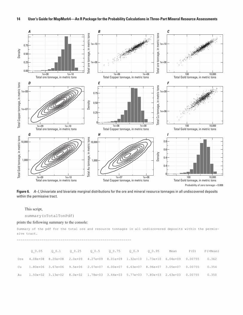
Another way to analyze this pdf is to plot each of the univariate and bivariate marginal distributions. These plots can be arranged in a matrix using this script:
plotMarginals(oTotalTonPdf)
The resulting matrix of plots is shown in figure 6. Above the matrix, the probability of zero tonnage is printed. The matrix has three parts—the plots in the upper triangle, the plots along the diagonal, and the plots in the lower triangle. In the upper triangle are crossplots of the ore and mineral resource tonnages, showing the bivariate marginal distributions. Along the diagonal are histograms, showing the univariate marginal distributions. In the lower triangle are contour plots, showing the bivariate marginal distributions. The plots in the lower triangle have corresponding plots in the upper triangle. The bivariate distributions show that the ore and mineral resource tonnages are highly correlated, which is common.
0.75
0.75
0.25
0
0.50
1.00
0.50
0.25
0
A
B
Probability of zerotonnage = 0.008
1e+02 1e+06 1e+10
1e+02 1e+05 1e+08 1e+11
Total tonnage, in metric tons
Dens
ityPr
obab
ility
Material
EXPLANATION
Ore
Copper
Gold
Figure 5. A, Univariate, marginal, probability density functions and B, univariate, marginal, complementary cumulative distribution functions for the total ore and mineral resource tonnages in all undiscovered deposits within the permissive tract.
DEN0041_fig_05\\IGSKAHCMVSFS002\Pubs_Common\Jeff\den17_cmrp00_0041_tm_ellefson\report_figures
14 User’s Guide for MapMark4—An R Package for the Probability Calculations in Three-Part Mineral Resource Assessments
This script,
summary(oTotalTonPdf)
prints the following summary to the console:Summary of the pdf for the total ore and resource tonnages in all undiscovered deposits within the permis-
sive tract.
------------------------------------------------------------
Ore
Q_0.05
4.08e+08
Q_0.1
8.20e+08
Q_0.25
2.0e+09
Q_0.5
4.27e+09
Q_0.75
8.01e+09
Q_0.9
1.32e+10
Q_0.95
1.73e+10
Mean
6.04e+09
P(0)
0.00755
P(>Mean)
0.362
Cu 1.80e+06 3.67e+06 9.5e+06 2.07e+07 4.00e+07 6.63e+07 8.96e+07 3.05e+07 0.00755 0.354
Au 1.50e+02 3.13e+02 8.0e+02 1.78e+03 3.44e+03 5.77e+03 7.80e+03 2.63e+03 0.00755 0.350
DEN0041_fig_06\\IGSKAHCMVSFS002\Pubs_Common\Jeff \den17_cmrp00_0041_tm_ellefson\report_figures
Probability of zero tonnage = 0.008
Total ore tonnage, in metric tons
Tota
l ore
tonn
age,
in m
etric
tons
Tota
l ore
tonn
age,
in m
etric
tons
0.00
0.25
0.50
0.75
Dens
ity
0.50
0.75
0.25
0
Dens
ity
0.8
0.6
0.4
0.4
0
Dens
ity
Tota
l Cop
per t
onna
ge, i
n m
etric
tons
Tota
l Gol
d to
nnag
e, in
met
ric to
ns
1e+07
1e+08
Tota
l Cu
tonn
age,
in m
etric
tons
1e+06
1e+08
BA C
D E F
G H I
1,000
10,000
Tota
l Au
tonn
age,
in m
etric
tons
1,000
10,000
1e+08 1e+10
Total ore tonnage, in metric tons1e+09 1e+10
Total ore tonnage, in metric tons1e+09 1e+10
Total Copper tonnage, in metric tons1e+06 1e+08
Total Copper tonnage, in metric tons1e+06 1e+08
Total Copper tonnage, in metric tons1e+07 1e+08
Total Gold tonnage, in metric tons100 10,000
Total Gold tonnage, in metric tons100 10,000
Total Gold tonnage, in metric tons100 10,000
1e+08
1e+10
1e+08
1e+10
Figure 6. A–I, Univariate and bivariate marginal distributions for the ore and mineral resource tonnages in all undiscovered deposits within the permissive tract.
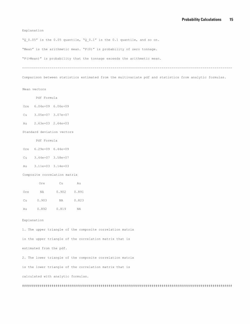
Probability Calculations 15
Explanation
“Q_0.05” is the 0.05 quantile, “Q_0.1” is the 0.1 quantile, and so on.
“Mean” is the arithmetic mean. “P(0)” is probability of zero tonnage.
“P(>Mean)” is probability that the tonnage exceeds the arithmetic mean.
-----------------------------------------------------------------------------------------------------------
Comparison between statistics estimated from the multivariate pdf and statistics from analytic formulas.
Mean vectors
Pdf Formula
Ore 6.04e+09 6.06e+09
Cu 3.05e+07 3.07e+07
Au 2.63e+03 2.64e+03
Standard deviation vectors
Pdf Formula
Ore 6.29e+09 6.44e+09
Cu 3.44e+07 3.58e+07
Au 3.11e+03 3.14e+03
Composite correlation matrix
Ore Cu Au
Ore NA 0.902 0.891
Cu 0.903 NA 0.823
Au 0.892 0.819 NA
Explanation
1. The upper triangle of the composite correlation matrix
is the upper triangle of the correlation matrix that is
estimated from the pdf.
2. The lower triangle of the composite correlation matrix
is the lower triangle of the correlation matrix that is
calculated with analytic formulas.
###########################################################################################################
16 User’s Guide for MapMark4—An R Package for the Probability Calculations in Three-Part Mineral Resource Assessments
The last part of the summary is a comparison between two sets of statistics. One set is estimated from the random samples that implicitly define the pdf for total ore and mineral resource tonnage in the permissive tract. This set is labeled “Pdf” in the sum-mary. The other set is calculated with analytic formulas, which are described in Ellefsen (2017). This set is labeled “Formula” in this summary. This comparison is important because it is a test of the simulation and the distribution for the total ore and mineral resource tonnage. If these two are performed properly, corresponding statistics should be similar, as they are in this example.
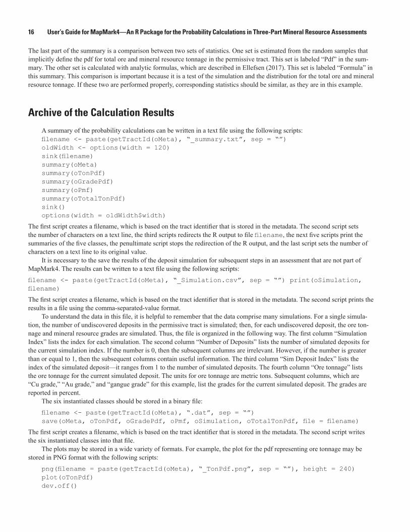
Archive of the Calculation Results
A summary of the probability calculations can be written in a text file using the following scripts:filename <- paste(getTractId(oMeta), “_summary.txt”, sep = “”)oldWidth <- options(width = 120)sink(filename)summary(oMeta)summary(oTonPdf)summary(oGradePdf)summary(oPmf)summary(oTotalTonPdf)sink()options(width = oldWidth$width)
The first script creates a filename, which is based on the tract identifier that is stored in the metadata. The second script sets the number of characters on a text line, the third scripts redirects the R output to file filename, the next five scripts print the summaries of the five classes, the penultimate script stops the redirection of the R output, and the last script sets the number of characters on a text line to its original value.
It is necessary to the save the results of the deposit simulation for subsequent steps in an assessment that are not part of MapMark4. The results can be written to a text file using the following scripts:
filename <- paste(getTractId(oMeta), “_Simulation.csv”, sep = “”) print(oSimulation, filename)
The first script creates a filename, which is based on the tract identifier that is stored in the metadata. The second script prints the results in a file using the comma-separated-value format.
To understand the data in this file, it is helpful to remember that the data comprise many simulations. For a single simula-tion, the number of undiscovered deposits in the permissive tract is simulated; then, for each undiscovered deposit, the ore ton-nage and mineral resource grades are simulated. Thus, the file is organized in the following way. The first column “Simulation Index” lists the index for each simulation. The second column “Number of Deposits” lists the number of simulated deposits for the current simulation index. If the number is 0, then the subsequent columns are irrelevant. However, if the number is greater than or equal to 1, then the subsequent columns contain useful information. The third column “Sim Deposit Index” lists the index of the simulated deposit—it ranges from 1 to the number of simulated deposits. The fourth column “Ore tonnage” lists the ore tonnage for the current simulated deposit. The units for ore tonnage are metric tons. Subsequent columns, which are “Cu grade,” “Au grade,” and “gangue grade” for this example, list the grades for the current simulated deposit. The grades are reported in percent.
The six instantiated classes should be stored in a binary file:
filename <- paste(getTractId(oMeta), “.dat”, sep = “”)save(oMeta, oTonPdf, oGradePdf, oPmf, oSimulation, oTotalTonPdf, file = filename)
The first script creates a filename, which is based on the tract identifier that is stored in the metadata. The second script writes the six instantiated classes into that file.
The plots may be stored in a wide variety of formats. For example, the plot for the pdf representing ore tonnage may be stored in PNG format with the following scripts:
png(filename = paste(getTractId(oMeta), “_TonPdf.png”, sep = “”), height = 240)plot(oTonPdf)dev.off()
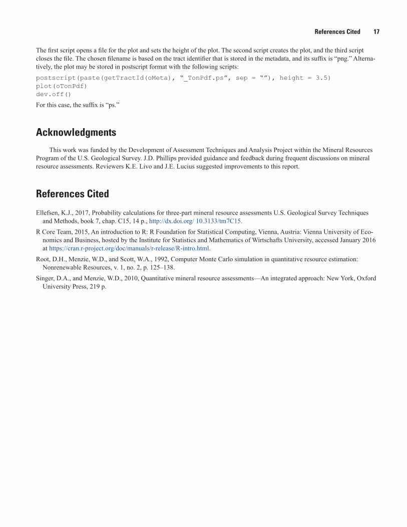
References Cited 17
The first script opens a file for the plot and sets the height of the plot. The second script creates the plot, and the third script closes the file. The chosen filename is based on the tract identifier that is stored in the metadata, and its suffix is “png.” Alterna-tively, the plot may be stored in postscript format with the following scripts:postscript(paste(getTractId(oMeta), “_TonPdf.ps”, sep = “”), height = 3.5)plot(oTonPdf)dev.off()
For this case, the suffix is “ps.”
AcknowledgmentsThis work was funded by the Development of Assessment Techniques and Analysis Project within the Mineral Resources
Program of the U.S. Geological Survey. J.D. Phillips provided guidance and feedback during frequent discussions on mineral resource assessments. Reviewers K.E. Livo and J.E. Lucius suggested improvements to this report.
References Cited
Ellefsen, K.J., 2017, Probability calculations for three-part mineral resource assessments U.S. Geological Survey Techniques and Methods, book 7, chap. C15, 14 p., http://dx.doi.org/ 10.3133/tm7C15.
R Core Team, 2015, An introduction to R: R Foundation for Statistical Computing, Vienna, Austria: Vienna University of Eco-nomics and Business, hosted by the Institute for Statistics and Mathematics of Wirtschafts University, accessed January 2016 at https://cran.r-project.org/doc/manuals/r-release/R-intro.html.
Root, D.H., Menzie, W.D., and Scott, W.A., 1992, Computer Monte Carlo simulation in quantitative resource estimation: Nonrenewable Resources, v. 1, no. 2, p. 125–138.
Singer, D.A., and Menzie, W.D., 2010, Quantitative mineral resource assessments—An integrated approach: New York, Oxford University Press, 219 p.

Appendix 1. Probability Calculations for a Tonnage Model 19
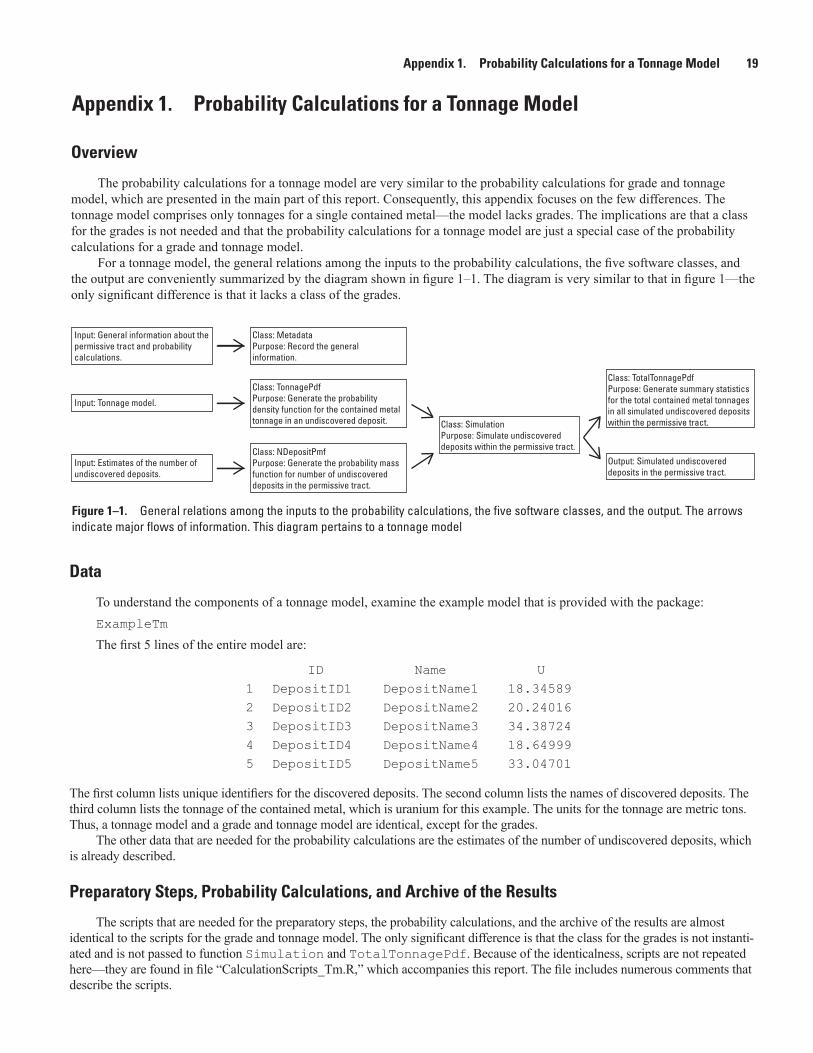
Appendix 1. Probability Calculations for a Tonnage Model
Overview
The probability calculations for a tonnage model are very similar to the probability calculations for grade and tonnage model, which are presented in the main part of this report. Consequently, this appendix focuses on the few differences. The tonnage model comprises only tonnages for a single contained metal—the model lacks grades. The implications are that a class for the grades is not needed and that the probability calculations for a tonnage model are just a special case of the probability calculations for a grade and tonnage model.
For a tonnage model, the general relations among the inputs to the probability calculations, the five software classes, and the output are conveniently summarized by the diagram shown in figure 1–1. The diagram is very similar to that in figure 1—the only significant difference is that it lacks a class of the grades.
Data
To understand the components of a tonnage model, examine the example model that is provided with the package:ExampleTm
The first 5 lines of the entire model are:
DEN0041_fig_A1_01\\IGSKAHCMVSFS002\Pubs_Common\Jeff\den17_cmrp00_0041_tm_ellefson\report_figures
ID Name U12345
DepositID1DepositID2DepositID3DepositID4DepositID5
DepositName1DepositName2DepositName3DepositName4DepositName5
18.3458920.2401634.3872418.6499933.04701
The first column lists unique identifiers for the discovered deposits. The second column lists the names of discovered deposits. The third column lists the tonnage of the contained metal, which is uranium for this example. The units for the tonnage are metric tons. Thus, a tonnage model and a grade and tonnage model are identical, except for the grades.
The other data that are needed for the probability calculations are the estimates of the number of undiscovered deposits, which is already described.
Preparatory Steps, Probability Calculations, and Archive of the Results
The scripts that are needed for the preparatory steps, the probability calculations, and the archive of the results are almost identical to the scripts for the grade and tonnage model. The only significant difference is that the class for the grades is not instanti-ated and is not passed to function Simulation and TotalTonnagePdf. Because of the identicalness, scripts are not repeated here—they are found in file “CalculationScripts_Tm.R,” which accompanies this report. The file includes numerous comments that describe the scripts.
Input: General information about thepermissive tract and probability calculations.
Class: MetadataPurpose: Record the generalinformation.
Class: SimulationPurpose: Simulate undiscovereddeposits within the permissive tract.
Class: TonnagePdfPurpose: Generate the probabilitydensity function for the contained metal tonnage in an undiscovered deposit.
Class: TotalTonnagePdfPurpose: Generate summary statisticsfor the total contained metal tonnagesin all simulated undiscovered depositswithin the permissive tract.
Class: NDepositPmfPurpose: Generate the probability massfunction for number of undiscovereddeposits in the permissive tract.
Input: Estimates of the number ofundiscovered deposits.
Output: Simulated undiscovereddeposits in the permissive tract.
Input: Tonnage model.
Figure 1–1. General relations among the inputs to the probability calculations, the five software classes, and the output. The arrows indicate major flows of information. This diagram pertains to a tonnage model

Appendix 2. Custom Distribution for the Number of Undiscovered Deposits 21
Appendix 2. Custom Distribution for the Number of Undiscovered Deposits
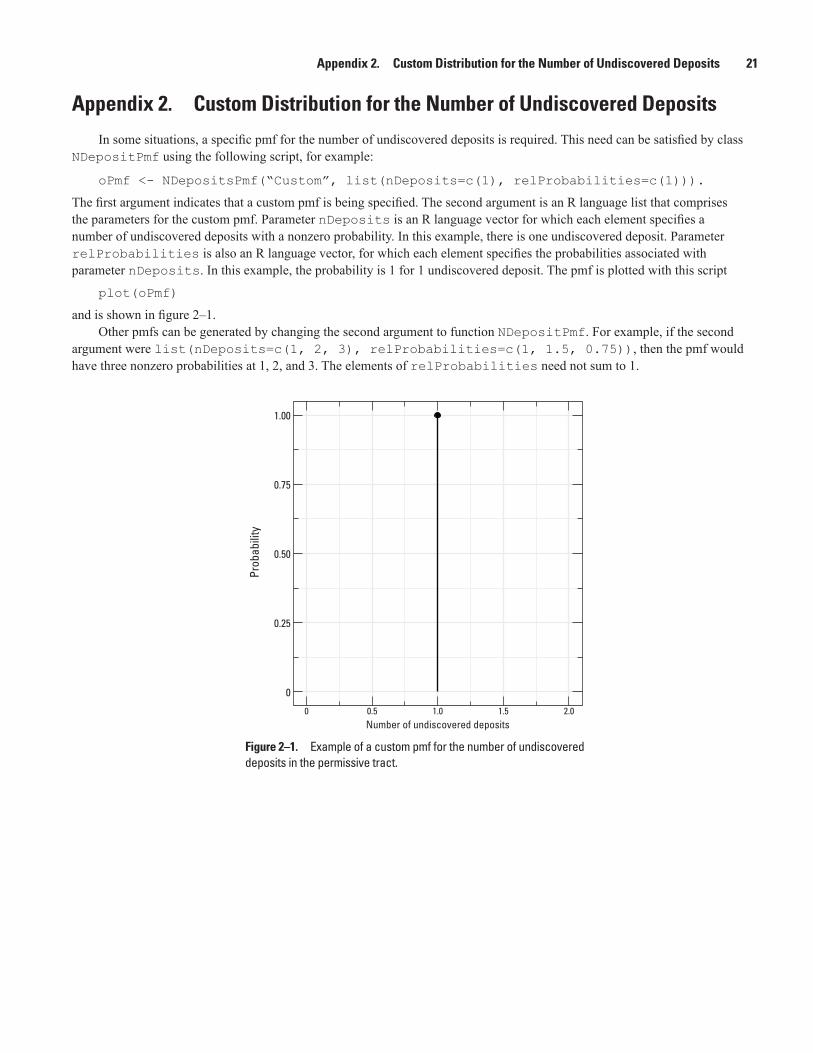
In some situations, a specific pmf for the number of undiscovered deposits is required. This need can be satisfied by class NDepositPmf using the following script, for example:
oPmf <- NDepositsPmf(“Custom”, list(nDeposits=c(1), relProbabilities=c(1))).
The first argument indicates that a custom pmf is being specified. The second argument is an R language list that comprises the parameters for the custom pmf. Parameter nDeposits is an R language vector for which each element specifies a number of undiscovered deposits with a nonzero probability. In this example, there is one undiscovered deposit. Parameter relProbabilities is also an R language vector, for which each element specifies the probabilities associated with parameter nDeposits. In this example, the probability is 1 for 1 undiscovered deposit. The pmf is plotted with this script
plot(oPmf)
and is shown in figure 2–1.Other pmfs can be generated by changing the second argument to function NDepositPmf. For example, if the second
argument were list(nDeposits=c(1, 2, 3), relProbabilities=c(1, 1.5, 0.75)), then the pmf would have three nonzero probabilities at 1, 2, and 3. The elements of relProbabilities need not sum to 1.
DEN0041_fig_A2_01\\IGSKAHCMVSFS002\Pubs_Common\Jeff\den17_cmrp00_0041_tm_ellefson\report_figures
0 0.5 1.0 1.5 2.0Number of undiscovered deposits
Prob
abili
ty
0
0.25
0.50
0.75
1.00
Figure 2–1. Example of a custom pmf for the number of undiscovered deposits in the permissive tract.

Appendix 4. Calculation Scripts 23
Appendix 3. Installation Instructions
Please see the file that accompanies this report, “InstallationInstructions.txt.”
Required Packages
Package MapMark4 requires packages compositions, mvtnorm, ks, and ggplot2. These packages are available from the R package repository and should be installed first. The latest versions of these packages are required for proper function of the package MapMark4. Also, Rtools (https://cran.r-project.org/bin/windows/Rtools/) is required during the install.
Installation Instructions for MapMark4 When Using RStudio
1. On the menu bar, click on “Tools” and then click on “Install Packages.” The Install-Packages window will appear. 2. Under item “Install from:” select “Package Archive File (.zip; .tar.gz).” Under item “Package archive,” use the Browse
button to locate file “MapMark4_1.0.tar.gz.” If you use multiple libraries, then you must select the appropriate library for the installation, using item “Install to Library.” Otherwise, use the default value in this item. Finally, click on “Install.”
Installation Instructions for MapMark4 When Using RGui
1. In the R console window, type “setwd(directory)” where “directory” is the directory containing the file “MapMark4_1.0.tar.gz.” Two backslashes (“\\”) are needed to separate folders within argument directory. For example, if the directory is F:\temp\install, then argument directory should be “F:\\temp\\install”
2. Type “install.packages(‘MapMark4_1.0.tar.gz’)”, and the package will be installed in the default library.
Appendix 4. Calculation ScriptsCopies of the scripts in this User’s Guide are stored in files “CalculationScripts_Gatm.R” and “CalculationScripts_Tm.R”
that accompany this report.
Publishing support provided by: Denver Publishing Service Center, Denver, Colorado
For more information concerning this publication, contact:
Center Director, USGS Crustal Geophysics and Geochemistry Science Center Box 25046, Mail Stop 964 Denver, CO 80225 (303) 236-1312
Or visit the Crustal Geophysics and Geochemistry Science Center Web site at: https://crustal.usgs.gov/
This publication is available online at: https://doi.org/10.3133/tm7C14

Ellefsen, K.J.—User’s Guide for M
apMark4—
An R Package for the Probability Calculations in Three-Part M
ineral Resource Assessm
ents—Techniques and M
ethods 7–C14ISSN 2328-7055 (online)https://doi.org/10.3133/tm7C14