Chapter 13 of Rojas Neural Networks a Systematic Introductionpage.mi.fu-berlin.de/rojas/neural/chapter/K13.pdf · state update. We adopt the additional simpliﬁcation that the state

13

The Hopfield Model

One of the milestones for the current renaissance in the field of neural networkswas the associative model proposed by Hopfield at the beginning of the 1980s.Hopfield’s approach illustrates the way theoretical physicists like to thinkabout ensembles of computing units. No synchronization is required, eachunit behaving as a kind of elementary system in complex interaction with therest of the ensemble. An energy function must be introduced to harness thetheoretical complexities posed by such an approach. The next two sectionsdeal with the structure of Hopfield networks. We then proceed to show thatthe model converges to a stable state and that two kinds of learning rules canbe used to find appropriate network weights.

13.1 Synchronous and asynchronous networks

A relevant issue for the correct design of recurrent neural networks is the ad-equate synchronization of the computing elements. In the case of McCulloch-Pitts networks we solved this difficulty by assuming that the activation of eachcomputing element consumes a unit of time. The network is built taking thisdelay into account and by arranging the elements and their connections in thenecessary pattern. When the arrangement becomes too contrived, additionalunits can be included which serve as delay elements. What happens whenthis assumption is lifted, that is, when the synchronization of the computingelements is eliminated?

13.1.1 Recursive networks with stochastic dynamics

We discussed the design and operation of associative networks in the previouschapter. The synchronization of the output was achieved by requiring that allcomputing elements evaluate their inputs and compute their output simulta-neously. Under this assumption the operation of the associative memory can

R. Rojas: Neural Networks, Springer-Verlag, Berlin, 1996R. Rojas: Neural Networks, Springer-Verlag, Berlin, 1996

R. Rojas: Neural Networks, Springer-Verlag, Berlin, 1996

338 13 The Hopfield Model

be described with simple linear algebraic methods. The excitation of the out-put units is computed using vector-matrix multiplication and evaluating thesign function at each node.

The methods we have used before to avoid dealing explicitly with thesynchronization problem have the disadvantage, from the point of view of bothbiology and physics, that global information is needed, namely a global time.Whereas in conventional computers synchronization of the digital buildingblocks is achieved using a clock signal, there is no such global clock in biologicalsystems. In a more biologically oriented simulation, global synchronizationshould thus be avoided. In this chapter we deal with the problem of identifyingthe properties of neural networks lacking global synchronization.

Networks in which the computing units are activated at different timesand which provide a computation after a variable amount of time are stochas-tic automata. Networks built from this kind of units behave like stochasticdynamical systems.

13.1.2 The bidirectional associative memory

Before we start analyzing asynchronous networks we will examine anotherkind of synchronous associative model with bidirectional edges. We will arriveat the concept of the energy function in a very natural way.

We have already discussed recurrent associative networks in which theoutput of the network is fed back to the input units using additional feed-back connections (Figure 12.3). In this way we designed recurrent dynamicalsystems and tried to determine their fixpoints. However, there is another wayto define a recurrent associative memory made up of two layers which sendinformation recursively between them. The input layer contains units whichreceive the input to the network and send the result of their computationto the output layer. The output of the first layer is transported by bidirec-tional edges to the second layer of units, which then return the result of theircomputation back to the first layer using the same edges. As in the case ofassociative memory models, we can ask whether the network achieves a stablestate in which the information being sent back and forth does not change aftera few iterations [258]. Such a network (shown in Figure 13.1) is known as aresonance network or bidirectional associative memory (BAM). The activa-tion function of the units is the sign function and information is coded usingbipolar values.

The network in Figure 13.1 maps an n-dimensional row vector x0 to a k-dimensional row vector y0. We denote the n×k weight matrix of the networkby W so that the mapping computed in the first step can be written as

y0 = sgn(x0W).

In the feedback step y0 is treated as the input and the new computation is

xT1 = sgn(WyT

0 ).



13.1 Synchronous and asynchronous networks 339

x1

x2

x3

xn

y1

y2

y3

yk

w11

wnk

.

.

.

.

.

.

Fig. 13.1. Example of a resonance network (BAM)

A new computation from left to right produces

y1 = sgn(x1W).

After m iterations the system has computed a set of m + 1 vector pairs(x0,y0), . . . , (xm,ym) which fulfill the conditions

yi = sgn(xiW) (13.1)

andxT

i+1 = sgn(WyTi ). (13.2)

The question is whether after some iterations a fixpoint (x,y) is found. Thisis the case when both

y = sgn(xW) and xT = sgn(WyT) (13.3)

hold. The BAM is thus a generalization of a unidirectional associative memory.An input vector, the “key”, can be presented to the network from the left orfrom the right and, after some iterations, the BAM finds the correspondingcomplementary vector. As can be seen, no external feedback connections arenecessary. The same edges are used for the transmission of information backand forth.

It can be immediately deduced from (13.3) that if a vector pair (x,y) isgiven and we want to condition a BAM to accept this pair as a fixed point,Hebbian learning can be used to compute an adequate matrix W. If W isdefined as W = xTy, as prescribed by Hebbian learning, then

y = sgn(xW) = sgn(xxTy) = sgn(‖x‖2y) = y

and also

xT = sgn(WyT) = sgn(xTyyT) = sgn(xT‖y‖2) = xT.




If we want to store several vector pairs (x1,y1), . . . , (xm,ym) in a BAM, thenHebbian learning works better if the vectors x1, . . . ,xm and y1, . . . ,ym arepairwise orthogonal within their respective groups, because in that case theperturbation term becomes negligible (refer to Chap. 12).

For a set of m vector pairs the matrix W is set to

W = xT1 y1 + xT

2 y2 + · · ·+ xTmym.

BAMs can be used to build autoassociative networks because the matricesproduced by the Hebb rule or by computing the pseudoinverse are symmetric.To see this, define X as the matrix, each of whose m rows is an n-dimensionalvector, so that if W denotes the connection matrix of an autoassociativememory for those m vectors, then it is true that

X = XW and XT = WXT,

because W is symmetric. This is just another way of writing the type ofcomputation performed by a BAM.

13.1.3 The energy function

With the BAM we can motivate and explore the concept of an energy functionin a simple setting. Assume that a BAM is given for which the vector pair(x,y) is a stable state. If the initial vector presented to the network fromthe left is x0, the network will converge to (x,y) after some iterations. Thevector y0 is computed according to y0 = sgn(x0W). If y0 is now used for anew iteration from the right, excitation of the units in the left layer can besummarized in an excitation vector e computed according to

eT = Wy0.

The vector pair (x0,y0) is a stable state of the network if sgn(e) = x0. Allvectors e close enough to x0 fulfill this condition. These vectors differ fromx0 by a small angle and therefore the product x0eT is larger than for othervectors of the same length but further away from x0. The product

E = −x0eT = −x0WyT0

is therefore smaller (because of the minus sign) if the vector WyT0 lies closer

to x0. The scalar value E can be used as a kind of index of convergence tothe stable states of an associative memory. We call E the energy function ofthe network.

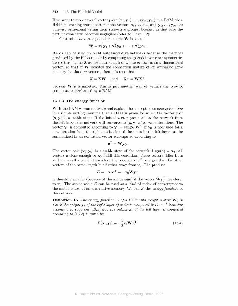
Definition 16. The energy function E of a BAM with weight matrix W, inwhich the output yi of the right layer of units is computed in the i-th iterationaccording to equation (13.1) and the output xi of the left layer is computedaccording to (13.2) is given by

E(xi,yi) = −12xiWyT

i . (13.4)



13.2 Definition of Hopfield networks 341

The factor 1/2 will be useful later and is just a scaling constant for theenergy function. In the following sections we show that the energy functionassumes locally minimal values at stable states. The energy function can alsobe generalized to arbitrary vectors x and y.

Up to this point we have only considered units with the sign function asactivation nonlinearity in the type of associative memories we have discussed.If we now consider units with a threshold and the step function as its activationfunction, we must use a more general expression for the energy function.This can be done by extending the input vectors with an additional constantcomponent. Each n-dimensional vector x will be transformed into the vector(x1, . . . , xn, 1). We proceed in a similar way with the k-dimensional vectory. The weight matrix W must be extended to a new matrix W′ with anadditional row and column. The negative thresholds of the units in the rightlayer of the BAM are included in row n + 1 of W′, whereas the negativethresholds of the units in the left are used as the entries of the column k + 1of the weight matrix. The entry (n+ 1, k+ 1) of the weight matrix can be setto zero. This transformation is equivalent to the introduction of an additionalunit with constant output 1 into each layer. The weight of each edge froma constant unit to each one of the others is the negative threshold of theconnected unit. It is straightforward to deduce that the energy function ofthe extended network can be written as

E(xi,yi) = −12xiWyT

i +12θryT

i +12xiθ

T� . (13.5)

The row vector of thresholds of the k units in the left layer is denoted in theabove expression by θ�. The row vector of thresholds of the n units in theright layer is denoted by θr.

13.2 Definition of Hopfield networks

So far we have considered only conventional or bidirectional associative mem-ories working with synchronized units. Dropping the assumption of simultane-ous firing of the computing elements leads to the appearance of novel networkproperties.

13.2.1 Asynchronous networks

In an asynchronous network each unit computes its excitation at random timesand changes its state to 1 or −1 independently of the others and according tothe sign of its total excitation. The probability of two units firing simultane-ously is zero. Consequently, the same dynamics can be obtained by selectingone unit randomly, computing its excitation and updating its state accord-ingly. There will not be any delay between computation of the excitation andstate update. We adopt the additional simplification that the state of a unit




is not changed if the total excitation is zero. This means that we leave thesign function undefined for the argument zero. Asynchronous networks areof course more realistic models of biological networks, although the assump-tion of zero delay in the computation and transmission of signals lacks anybiological basis.

Using the energy function it can be shown that a BAM arrives at a stablestate after a finite number of iterations. A stable state is a vector pair (x,y)which fulfills the conditions (13.3). When a BAM reaches this state pair, nocomponent of the bipolar vectors x and y can be changed without contra-dicting (13.3). The vector pair (x,y) is therefore also a stable state for anasynchronous network.

Proposition 19. A bidirectional associative memory with an arbitrary weightmatrix W reaches a stable state in a finite number of iterations using eithersynchronous or asynchronous updates.

Proof. For a vector x = (x1, x2, . . . , xn), a vector y = (y1, y2, . . . , yk) and ann× k weight matrix W = {wij} the energy function is the bilinear form

E(x,y) = −12(x1, x2, . . . , xn)

⎛⎜⎜⎜⎝w11 w12 · · · w1k

w21 w22 · · · w2k

.... . .

...wn1 wn2 · · · wnk

⎞⎟⎟⎟⎠⎛⎜⎜⎜⎝y1y2...yk

⎞⎟⎟⎟⎠ .

The value of E(x,y) can be computed by multiplying first W by yT and theresult with −x/2. The product of the i-th row of W and yT represents theexcitation of the i-th unit in the left layer. If we denote these excitations byg1, g2, . . . , gn the above expression transforms to

E(x,y) = −12(x1, x2, . . . , xn)

⎛⎜⎜⎜⎝g1g2...gn

⎞⎟⎟⎟⎠ .

We can also compute E(x,y) multiplying first x by W. The product of the i-thcolumn of W with x corresponds to the excitation of unit i in the right layer.If we denote these excitations by e1, e2, . . . , ek, the expression for E(x,y) canbe written as

E(x,y) = −12(e1, e2, . . . , ek)

⎛⎜⎜⎜⎝y1y2...yk

⎞⎟⎟⎟⎠ .

Therefore, the energy function can be written in the two equivalent forms

E(x,y) = −12

k∑i=1

eiyi and E(x,y) = −12

n∑i=1

gixi.




In asynchronous networks at each time t we randomly select a unit from theleft or right layer. The excitation is computed and its sign is the new activationof the unit. If the previous activation of the unit remains the same after thisoperation, then the energy of the network has not changed.

The state of unit i on the left layer will change only when the excitation gi

has a different sign than xi, the present state. The state is updated from xi tox′i, where x′i now has the same sign as gi. Since the other units do not changetheir state, the difference between the previous energy E(x,y) and the newenergy E(x′,y) is

E(x,y) − E(x′,y) = −12gi(xi − x′i).

Since both xi and −xi have a different sign than gi it follows that

E(x,y) − E(x′,y) > 0.

The new state (x′,y) has a lower energy than the original state (x,y). Thesame argument can be made if a unit on the right layer has been selected, sothat for the new state (x,y′) it holds that

E(x,y) − E(x,y′) > 0,

whenever the state of a unit in the right layer has been flipped.Any update of the network state reduces the total energy. Since there are

only a finite number of possible combinations of bipolar states, the processmust stop at some point, that is, a state (a,b) is found whose energy cannotbe further reduced. The network has fallen into a local minimum of the energyfunction and the state (a,b) is an attractor of the system. �

The above proposition also holds for synchronous networks, since thesecan be considered as a special case of asynchronous dynamics. Note that theproposition puts conditions on the matrix W. This means that any given realmatrix W possesses bidirectional stable bipolar states.

13.2.2 Examples of the model

In 1982 the American physicist John Hopfield proposed an asynchronous neu-ral network model which made an immediate impact in the AI community. Itis a special case of a bidirectional associative memory, but chronologically itwas proposed before the BAM.

In the Hopfield model it is assumed that the individual units preservetheir individual states until they are selected for a new update. The selectionis made randomly. A Hopfield network consists of n totally coupled units,that is, each unit is connected to all other units except itself. The networkis symmetric because the weight wij for the connection between unit i and




unit j is equal to the weight wji of the connection from unit j to unit i. Thiscan be interpreted as meaning that there is a single bidirectional connectionbetween both units. The absence of a connection from each unit to itself avoidsa permanent feedback of its own state value [198].

Figure 13.2 shows an example of a network with three units. Each one ofthem can assume the state 1 or −1. A Hopfield network can also be interpretedas an asynchronous BAM in which the left and right layers of units have fusedto a single layer. The connections in a Hopfield network with n units can berepresented using an n× n weight matrix W = {wij} with a zero diagonal.

unit 3unit 2

unit 1

x3

x1

x2

w12 w13

w23

Fig. 13.2. A Hopfield network of three units

It is easy to show that if the weight matrix does not contain a zero diagonal,the network dynamics does not necessarily lead to stable states. The weightmatrix

W =

⎛⎝−1 0 0

0 −1 00 0 −1

⎞⎠ ,

for example, transforms the state vector (1, 1, 1) into the state vector(−1,−1,−1) and conversely. In the case of asynchronous updating, the net-work chooses randomly among the eight possible network states.

A connection matrix with a zero diagonal can also lead to oscillations inthe case where the weight matrix is not symmetric. The weight matrix

W =(

0 −11 0

)

describes the network of Figure 13.3. It transforms the state vector (1,−1)into the state vector (1, 1) when the network is running asynchronously. Afterthis transition the state (−1, 1) can be updated to (−1,−1) and finally to(1,−1). The state vector changes cyclically and does not converge to a stablestate.




1

–1

x1 x2

Fig. 13.3. Network with asymmetric connections

The symmetry of the weight matrix and a zero diagonal are thus necessaryconditions for the convergence of an asynchronous totally connected networkto a stable state. These conditions are also sufficient, as we show later.

The units of a Hopfield network can be assigned a threshold θ differentfrom zero. In this case each unit selected for a state update adopts the state1 if its total excitation is greater than θ, otherwise the state −1. This is theactivation rule for perceptrons, so that we can think of Hopfield networks asasynchronous recurrent networks of perceptrons.

The energy function of a Hopfield network composed of units with thresh-olds different from zero can be defined in a similar way as for the BAM. Inthis case the vector y of equation (13.5) is x and we let θ = θ� = θr.

Definition 17. Let W denote the weight matrix of a Hopfield network of nunits and let θ be the n-dimensional row vector of units’ thresholds. The energyE(x) of a state x of the network is given by

E(x) = −12xWxT + θxT.

The energy function can also be written in the form

E(x) = −12

n∑j=1

n∑i=1

wijxixj +n∑

i=1

θixi.

The factor 1/2 is used because the identical terms wijxixj and wjixjxi arepresent in the double sum.

The energy function of a Hopfield network is a quadratic form. A Hop-field network always finds a local minimum of the energy function. It is thusinteresting to look at an example of the shape of such an energy function. Fig-ure 13.4 shows a network of just two units with threshold zero. It is obviousthat the only stable states are (1,−1) and (−1, 1). In any other state, one ofthe units forces the other to change its state to stabilize the network. Sucha network is a flip-flop, a logic component with two outputs which assumecomplementary logic values.

The energy function of a flip-flop with weights w12 = w21 = −1 and twounits with threshold zero is given by

E(x1, x2) = x1x2,




0–1

0

Fig. 13.4. A flip-flop

where x1 and x2 denote the states of the first and second units respectively.Figure 13.5 shows the energy function for the so-called continuous Hopfieldmodel [199] in which the unit’s states can assume all real values between 0 and1. In the network of Figure 13.4 only the four discrete states (1, 1), (1,−1),(−1, 1) and (−1,−1) are allowed. The energy function has local minima at(1,−1) and (−1, 1). A flip-flop can therefore be interpreted as a network ca-pable of storing one of the states (1,−1) or (−1, 1).

-1

0

1 x1

-1

0

1

x2 -1

0

1

-1

0

1 x1

-1

0

1

x2 -1

0

1

Fig. 13.5. Energy function of a flip-flop

Hopfield networks can also be used to compute logical functions. Con-junction, for example, can be implemented with a network of three units. Thestates of two units are set and remain fixed during the computation (clampingtheir states). Only the third unit can change its state. If the network weightsand the unit thresholds have the appropriate values, the unconstrained unitwill assume a state which corresponds to the conjunction of the two clampedstates.

Figure 13.6 shows a network for the computation of the logical disjunctionof two Boolean values x1 and x2. The input is clamped and after some timethe network settles to a state which corresponds to the disjunction of x1 andx2. The constants “true” and “false” correspond to the numerical values 1and −1. In this network the thresholds of the clamped units and their mutualconnections play no role in the computation.




x1

x2

unit 3unit 2

unit 1

0.5

1

1–

Fig. 13.6. Network for the computation of the OR function

Since the individual units of the network are perceptrons, the question ofwhether there are logic functions which cannot be computed by a Hopfieldnetwork of a given size arises. This is the case in our next example. Assumethat a Hopfield network of three units should store the set of stable statesgiven by the following table:

unit 1 2 3state 1 −1 −1 −1state 2 1 −1 1state 3 −1 1 1state 4 1 1 −1

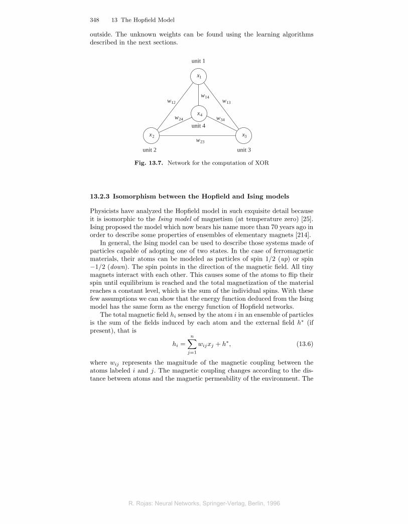
From the point of view of the third unit (third column) this is the XORfunction. If the four vectors shown above are to become stable states of thenetwork, the third unit cannot change state when any of these four vectorshas been loaded in the network. In this case the third unit should be capableof linearly separating the vectors (−1,−1) and (1, 1) from the vectors (−1, 1)and (1,−1), which we know is impossible. The same argument is valid forany of the three units, since the table given above remains unchanged aftera permutation of the units’ labels. This shows that no Hopfield network ofthree units can have these stable states. However, the XOR problem can besolved if the network is extended to four units. The network of Figure 13.7can assume the following stable states, if adequate weights and thresholds areselected:

unit 1 2 3 4state 1 −1 −1 −1 1state 2 1 −1 1 1state 3 −1 1 1 1state 4 1 1 −1 −1

The third column represents the XOR function of the two first columns. Thefourth column corresponds to an auxiliary unit, whose state can be set from




outside. The unknown weights can be found using the learning algorithmsdescribed in the next sections.

w12 w13

w23

unit 3unit 2

unit 1

unit 4

x3x2

x1

x4

w14

w24 w34

Fig. 13.7. Network for the computation of XOR

13.2.3 Isomorphism between the Hopfield and Ising models

Physicists have analyzed the Hopfield model in such exquisite detail becauseit is isomorphic to the Ising model of magnetism (at temperature zero) [25].Ising proposed the model which now bears his name more than 70 years ago inorder to describe some properties of ensembles of elementary magnets [214].

In general, the Ising model can be used to describe those systems made ofparticles capable of adopting one of two states. In the case of ferromagneticmaterials, their atoms can be modeled as particles of spin 1/2 (up) or spin−1/2 (down). The spin points in the direction of the magnetic field. All tinymagnets interact with each other. This causes some of the atoms to flip theirspin until equilibrium is reached and the total magnetization of the materialreaches a constant level, which is the sum of the individual spins. With thesefew assumptions we can show that the energy function deduced from the Isingmodel has the same form as the energy function of Hopfield networks.

The total magnetic field hi sensed by the atom i in an ensemble of particlesis the sum of the fields induced by each atom and the external field h∗ (ifpresent), that is

hi =n∑

j=1

wijxj + h∗, (13.6)

where wij represents the magnitude of the magnetic coupling between theatoms labeled i and j. The magnetic coupling changes according to the dis-tance between atoms and the magnetic permeability of the environment. The



13.3 Converge to stable states 349

external field

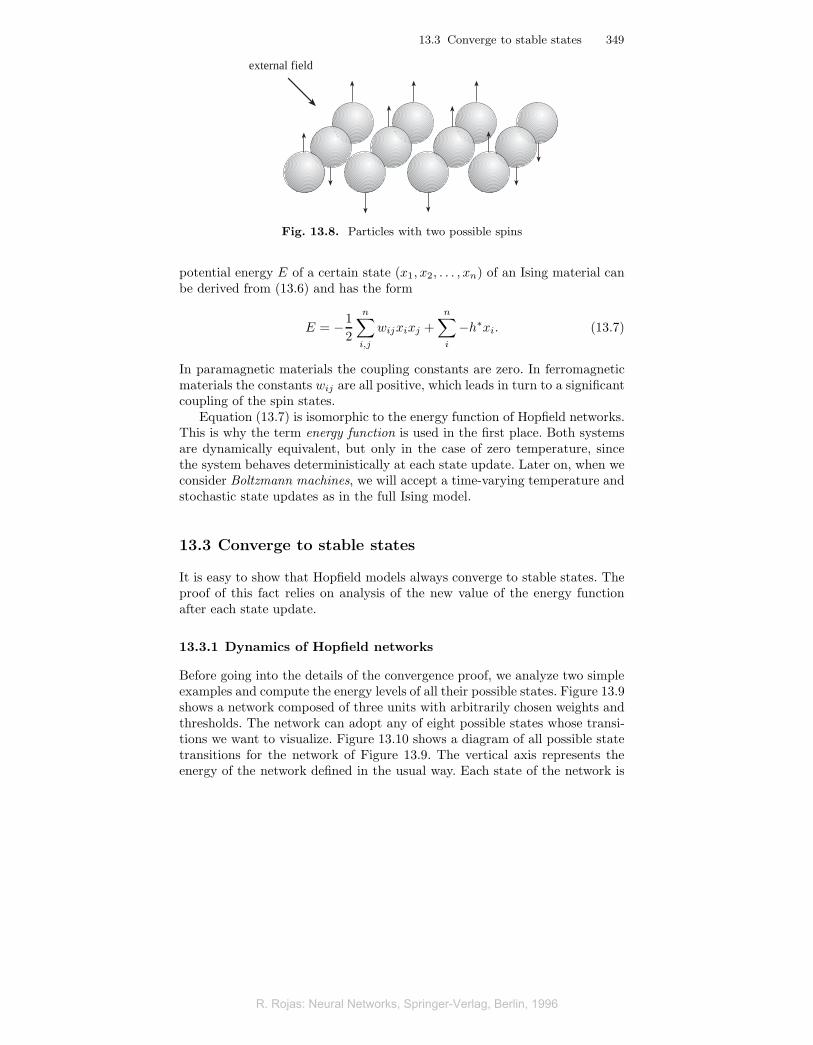
Fig. 13.8. Particles with two possible spins

potential energy E of a certain state (x1, x2, . . . , xn) of an Ising material canbe derived from (13.6) and has the form

E = −12

n∑i,j

wijxixj +n∑i

−h∗xi. (13.7)

In paramagnetic materials the coupling constants are zero. In ferromagneticmaterials the constants wij are all positive, which leads in turn to a significantcoupling of the spin states.

Equation (13.7) is isomorphic to the energy function of Hopfield networks.This is why the term energy function is used in the first place. Both systemsare dynamically equivalent, but only in the case of zero temperature, sincethe system behaves deterministically at each state update. Later on, when weconsider Boltzmann machines, we will accept a time-varying temperature andstochastic state updates as in the full Ising model.

13.3 Converge to stable states

It is easy to show that Hopfield models always converge to stable states. Theproof of this fact relies on analysis of the new value of the energy functionafter each state update.

13.3.1 Dynamics of Hopfield networks

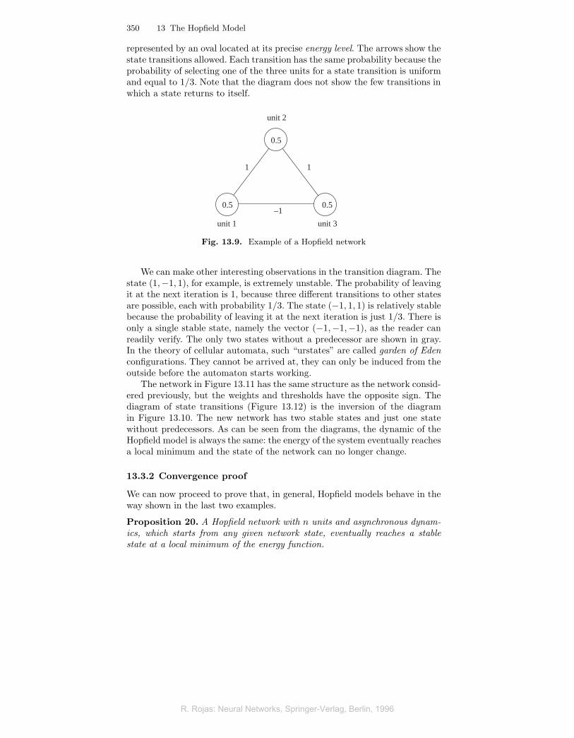
Before going into the details of the convergence proof, we analyze two simpleexamples and compute the energy levels of all their possible states. Figure 13.9shows a network composed of three units with arbitrarily chosen weights andthresholds. The network can adopt any of eight possible states whose transi-tions we want to visualize. Figure 13.10 shows a diagram of all possible statetransitions for the network of Figure 13.9. The vertical axis represents theenergy of the network defined in the usual way. Each state of the network is




represented by an oval located at its precise energy level. The arrows show thestate transitions allowed. Each transition has the same probability because theprobability of selecting one of the three units for a state transition is uniformand equal to 1/3. Note that the diagram does not show the few transitions inwhich a state returns to itself.

unit 3unit 1

unit 2

0.5

0.5 0.5

1 1

–1

Fig. 13.9. Example of a Hopfield network

We can make other interesting observations in the transition diagram. Thestate (1,−1, 1), for example, is extremely unstable. The probability of leavingit at the next iteration is 1, because three different transitions to other statesare possible, each with probability 1/3. The state (−1, 1, 1) is relatively stablebecause the probability of leaving it at the next iteration is just 1/3. There isonly a single stable state, namely the vector (−1,−1,−1), as the reader canreadily verify. The only two states without a predecessor are shown in gray.In the theory of cellular automata, such “urstates” are called garden of Edenconfigurations. They cannot be arrived at, they can only be induced from theoutside before the automaton starts working.

The network in Figure 13.11 has the same structure as the network consid-ered previously, but the weights and thresholds have the opposite sign. Thediagram of state transitions (Figure 13.12) is the inversion of the diagramin Figure 13.10. The new network has two stable states and just one statewithout predecessors. As can be seen from the diagrams, the dynamic of theHopfield model is always the same: the energy of the system eventually reachesa local minimum and the state of the network can no longer change.

13.3.2 Convergence proof

We can now proceed to prove that, in general, Hopfield models behave in theway shown in the last two examples.

Proposition 20. A Hopfield network with n units and asynchronous dynam-ics, which starts from any given network state, eventually reaches a stablestate at a local minimum of the energy function.




3.5

3.0

2.5

2.0

1.5

1.0

0.5

- 0.5

-1.0

-1.5

-2.0

-2.5

1 –1 1

1 1 1

–1 1 1

–1 –1 1

–1 –1 –1

–1 1 –1

1 1 –1

1 –1 –1

energy

stable state

Fig. 13.10. State transitions for the network of Figure 13.9

unit 3unit 1

unit 2

–1 –1

1

– 0.5

– 0.5 – 0.5

Fig. 13.11. Second example of a Hopfield network

Proof. The energy function of a state x = (x1, x2, . . . , xn) of a Hopfield net-work with n units is given by




2.5

2.0

1.5

1.0

0.5

-0.5

-1.0

- 1.5

-2.0

-2.5

-3.0

-3.5 1 –1 1

1 1 1

–1 1 1

–1 –1 1

–1 –1 –1

–1 1 –1

1 1 –1

1 –1 –1

energy

stable state

stable state

Fig. 13.12. State transitions for the network of Figure 13.11

E(x) = −12

n∑j=1

n∑i=1

wijxixj +n∑

i=1

θixi, (13.8)

where the terms involved are defined as usual. If during the current iterationunit k is selected and does not change its state, then the energy of the systemdoes not change either. If the state of the unit is changed in the updateoperation, the network reaches a new global state x′ = (x1, . . . , x

′k, . . . , xn)

for which the new energy is E(x′). The difference between E(x) and E(x′) isgiven by all terms in the summation in (13.8) which contain xk and x′k, thatis

E(x)− E(x′) = (−n∑

j=1

wkjxkxj + θkxk)− (−n∑

j=1

wkjx′kxj + θkx

′k).

The factor 1/2 disappears from the computation because the terms wkjxkxj

appear twice in the double sum of (13.8). Since wkk = 0 we can rewrite theabove equation as




E(x) − E(x′) = −(xk − x′k)n∑

j=1

wkjxj + θk(xk − x′k)

= −(xk − x′k)(n∑

j=1

wkjxj − θk),

from which we finally obtain

E(x) − E(x′) = −(xk − x′k)ek,

where ek denotes the total excitation of unit k (including subtraction of thethreshold). The excitation ek has a different sign from xk and −x′k, becauseotherwise the unit state would not have been changed. This means that theproduct −(xk − x′k)ek is positive and therefore

E(x)− E(x′) > 0.

This shows that every time the state of a unit is altered, the total energyof the network is reduced. Since there is only a finite set of possible states, thenetwork must eventually reach a state for which the energy cannot be reducedfurther. It is a stable state of the network, as we wanted to prove. �

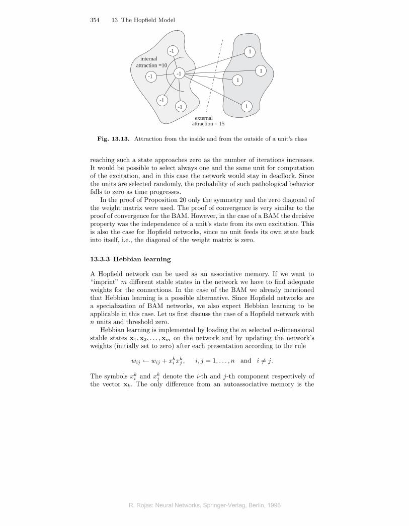
There is a simpler proof of the last proposition, which has the advantageof offering a nice visualization of the dynamics of a Hopfield network [74].Assume that we classify the units of a network according to their state: thefirst set contains the units with state 1, the second set the units with state−1. There are edges linking every unit with all the others, so that some edgesgo from one set to the other. We now randomly select one of the units andcompute its “attraction” by the units in its own set and the attraction by theunits in the other set. The “attraction” is the sum of the weights of all edgesbetween a unit and the units in its set or in the other one. If the attractionfrom the outside is greater than the attraction from its own set, the unitchanges sides by altering its state. If the external attraction is lower than theinternal, the unit keeps its current state. This procedure is repeated severaltimes, each time selecting one of the units randomly. It corresponds to theupdating strategy of a Hopfield network. Figure 13.13 shows an example inwhich the attraction from the outside is greater than the internal one. Theselected unit must change sides. It is clear that the network must eventuallyreach a stable state, because the sum of the weights of all edges connectingone set to the other can only become lower in the course of time. Since thenumber of possible network states is finite, a global state must be reached inwhich the attraction of one set by the other cannot be further reduced. Thisis the task known in combinatorics as the minimal cut problem, in which wewant to find a cut of minimal flow in a graph. The procedure described alwaysfinds a locally minimal cut.

The wording of Proposition 20 has been carefully chosen. That the net-work “eventually” settles in a stable state, means that the probability of not




-1

1-1 -1

-1-1

1

1

1

externalattraction = 15

internalattraction =10

Fig. 13.13. Attraction from the inside and from the outside of a unit’s class

reaching such a state approaches zero as the number of iterations increases.It would be possible to select always one and the same unit for computationof the excitation, and in this case the network would stay in deadlock. Sincethe units are selected randomly, the probability of such pathological behaviorfalls to zero as time progresses.

In the proof of Proposition 20 only the symmetry and the zero diagonal ofthe weight matrix were used. The proof of convergence is very similar to theproof of convergence for the BAM. However, in the case of a BAM the decisiveproperty was the independence of a unit’s state from its own excitation. Thisis also the case for Hopfield networks, since no unit feeds its own state backinto itself, i.e., the diagonal of the weight matrix is zero.

13.3.3 Hebbian learning

A Hopfield network can be used as an associative memory. If we want to“imprint” m different stable states in the network we have to find adequateweights for the connections. In the case of the BAM we already mentionedthat Hebbian learning is a possible alternative. Since Hopfield networks area specialization of BAM networks, we also expect Hebbian learning to beapplicable in this case. Let us first discuss the case of a Hopfield network withn units and threshold zero.

Hebbian learning is implemented by loading the m selected n-dimensionalstable states x1,x2, . . . ,xm on the network and by updating the network’sweights (initially set to zero) after each presentation according to the rule

wij ← wij + xki x

kj , i, j = 1, . . . , n and i �= j.

The symbols xki and xk

j denote the i-th and j-th component respectively ofthe vector xk. The only difference from an autoassociative memory is the




requirement of a zero diagonal. After presentation of the first vector x1 theweight matrix is given by the expression

W1 = xT1 x1 − I,

where I denotes the n× n identity matrix. Subtraction of the identity matrixguarantees that the diagonal of W becomes zero, since for any bipolar vectorxi it holds that xi

kxik = 1. Obviously W1 is a symmetric matrix.

The minimum of the energy function of a Hopfield network with the weightmatrix W1 is located at x1 because

E(x) = −12xW1xT = −1

2(xxT

1 x1xT − xxT)

and xxT = n for bipolar vectors. This means that the function

E(x) = −12‖xxT

1 ‖2 +n

2

has a local minimum at x = x1. In this case it holds that

E(x) = −n2

2+n

2.

This shows that x1 is a stable state of the network.In the case of m different vectors x1,x2, . . . ,xm the matrix W is defined

asW = (x1xT

1 − I) + (xT2 x2 − I) + · · ·+ (xT

mxm − I),

or equivalently

W = xT1 x1 + xT

2 x2 + · · ·+ xTmxm −mI.

If the network is initialized with the state x1, the vector e of the excitationof the units is

e = x1W

= x1xT1 x1 + x1xT

2 x2 + · · ·+ x1xTmxm −mx1I

= (n−m)x1 +m∑

j=2

α1jxj .

The constants α12, α13, . . . , α1m represent the scalar products of the first vec-tor with each one of the other m−1 vectors x2, . . . ,xm. The state x1 is stablewhen m < n and the perturbation term

∑mj=2 α1jxj is small. In this case it

holds thatsgn(e) = sgn(x1)

as desired. The same argumentation can be used for any of the other vec-tors. The best results are achieved with Hebbian learning when the vectorsx1,x2, . . . ,xm are orthogonal or close to orthogonal, just as in the case of anyother associative memory.




13.4 Equivalence of Hopfield and perceptron learning

Hebbian learning is a simple rule which is useful for the computation of theweight matrix in Hopfield networks. However, sometimes Hebbian learningcannot find a weight matrix for which m given vectors are stable states, al-though such a matrix exists. If the vectors to be stored lie near each other,the perturbation term can grow so large as to preclude a solution by Hebbianlearning. In this case another learning rule is needed, which is a variant ofperceptron learning.

13.4.1 Perceptron learning in Hopfield networks

Let us consider Hopfield networks composed of units with a non-zero thresholdand the step function as activation function. The units adopt state 1 whenthe excitation is greater than the threshold and otherwise the state −1. Theunits are just perceptrons and it is straightforward to assume that perceptronlearning could be used for determination of the weights and thresholds of thenetwork for a given learning problem.

Let n denote the number of units in a Hopfield network, let W = {wij}be the n × n weight matrix, and let θi denote the threshold of unit i. If avector x = (x1, . . . , xn) is given to be “imprinted” on the network, this vectorwill be a stable state only when, if loaded in the network, the network globalstate does not change. This is the case if for every unit its excitation minusits threshold has the same sign as the current state (the value zero is assignedthe minus sign). This means that the following n inequalities must hold:

For unit 1 : sgn(x1)(0 + x2w12 + x3w13 + · · ·+ xnw1n − θ1) < 0

For unit 2 : sgn(x2)(x1w21 + 0 + x3w23 + · · ·+ xnw2n − θ2) < 0

...For unit n : sgn(xn)(x1wn1 + x2wn2 + · · · + xn−1wnn−1

+ 0 − θn) < 0

The factor sgn(xi) is used in each inequality to obtain always the same in-equality operator (“less than”). Only the n(n − 1)/2 non-zero entries of theweight matrix as well as the n thresholds of the units appear in these inequal-ities. Let v denote a vector of dimension n + n(n − 1)/2 whose componentsare the non-diagonal entries wij of the weight matrix W (with i < j so as toconsider each weight only once) and the n thresholds with minus sign. Thevector v is given by

v = (w12, w13, . . . , w1n︸︷︷︸n−1

, w23, w24, . . . , w2n︸︷︷︸n−2

, . . . , wn−1n︸︷︷︸1

,−θ1, . . . ,−θn︸︷︷︸n

).



13.4 Equivalence of Hopfield and perceptron learning 357

The vector x is transformed into n auxiliary vectors z1, z2, . . . , zn of dimensionn+ n(n− 1)/2 given by the expression

z1 = (x2, x3, . . . , xn︸︷︷︸n−1

, 0, 0, . . . , 1, 0, . . . , 0︸︷︷︸n

)

z2 = (x1, 0, . . . , 0︸︷︷︸n−1

, x3, . . . , xn︸︷︷︸n−2

, 0, 0, . . . , 0, 1, . . . , 0︸︷︷︸n

)

...zn = (0, 0, . . . , x1︸︷︷︸

n−1

, 0, 0, . . . , x2︸︷︷︸n−2

, 0, 0, . . . , 0, 0, . . . , 1︸︷︷︸n

).

The components of the vectors z1, . . . , zn were defined so that the previousinequalities for each unit can be written in the equivalent form

unit 1 sgn(x1)z1 · v > 0unit 2 sgn(x2)z2 · v > 0...unit n sgn(xn)zn · v > 0

The vectors z1, z2, . . . , zn can always be defined in this way. We will not writedown the exact transformation rule here because it is rather involved.

The last set of inequalities shows that the solution to the original problemis found by computing a linear separation of the vectors z1, z2, . . . , zn. Thevectors which belong to the positive half-space are those for which sgn(xi)holds. The vectors which belong to the negative half-space are those for whichsgn(xi) = −1. This problem can be solved using perceptron learning, whichallows us to compute the vector v of weights needed for the linear separation,and from this we can deduce the weight matrix W.

In the case where m vectors x1,x2, . . . ,xm are given to be imprinted in theHopfield network, we have to use the above transformation for every one ofthem. Each vector is transformed into n auxiliary vectors, so that at the endwe have nm different auxiliary vectors which must be linearly separated. Ifthey are actually linearly separable, perceptron learning will find the solutionto the problem, coded in the vector v of the transformed perceptron.

The analysis performed above shows that it is possible to transform alearning problem in a Hopfield network with n units into a learning problemfor a perceptron of dimension n+n(n−1)/2, that is, n(n+1)/2. Figure 13.14shows an example of a Hopfield network that can be transformed into theequivalent perceptron to the right. The three-dimensional Hopfield problemis transformed in this way into a learning problem for a six-dimensional per-ceptron.

Each iteration of the perceptron learning algorithm updates only theweights of the edges attached to a single unit and its threshold. For example,if a correction is needed because of the sign of z1 · v, then only the weights




0w12 w13

w23

w12

w13

w23

θ1

θ2 θ3

−θ1

−θ2

−θ3

Fig. 13.14. Transformation of a Hopfield network into a perceptron

w12, w13, . . . , w1n and the threshold θ1 must be updated. This means that itis possible to use perceptron learning or the delta rule locally. During trainingall units are set to the desired stable states. If the sign of a unit’s excita-tion is incorrect for the desired state, then the weights and threshold of thisindividual perceptron are corrected in the usual manner. It is not necessaryto transform the Hopfield states into the n(n + 1)/2-dimensional perceptronstates every time we want to start the learning algorithm. This is only neededto prove the equivalence of Hopfield and perceptron learning.

13.4.2 Complexity of learning in Hopfield models

The interesting result which can immediately be inferred from the equivalenceof Hopfield networks and perceptrons is that every learning algorithm forperceptrons can be transformed into a learning method for Hopfield networks.The delta rule or algorithms that proceed by finding inner points of solutionpolytopes can also be used to train Hopfield networks.

We have already shown in Chap. 10 that learning problems for multilayernetworks are in general NP-complete. However, some special architecturescan be trained in polynomial time. We saw in Chap. 4 that the learning prob-lem for Hopfield networks can be solved in polynomial time, because thereare learning algorithms for perceptrons whose complexity grows polynomi-ally with the number of training vectors and their dimension (for example,Karmarkar’s algorithm). Since the transformation described in the previoussection converts m desired stable states into nm vectors to be linearly sep-arated, and since this can be done in polynomial time, it follows that thelearning problem for Hopfield networks can be solved in polynomial time. InChap. 6 we also showed how to compute an upper bound for the number oflinearly separable functions. This upper bound, valid for perceptrons, is alsovalid for Hopfield networks, since the stable states must be linearly separable(for the equivalent perceptron). This equivalence simplifies computation ofthe capacity of a Hopfield network when it is used as an associative memory.



13.5 Parallel combinatorics 359

13.5 Parallel combinatorics

The networks analyzed in the previous sections can be used either to computeBoolean functions or as associative memories. Those recurrent networks forwhich an energy function of a certain form exists can be used to solve somedifficult problems in the fields of combinatorics and optimization theory. Hop-field networks have been proposed for these kinds of tasks.

13.5.1 NP-complete problems and massive parallelism

Many complex problems can be solved in a reasonable length of time usingmultiprocessor systems and parallel algorithms. This is easier for tasks thatcan be divided into independent subproblems, which are then assigned todifferent processors. The solution to the original problem is obtained by col-lecting the partial results after they have been computed. However, many well-known and important problems cannot be split in this manner. The parallelprocesses must cooperate and exchange information, so that the programmermust include some synchronization primitives in the system. If synchroniza-tion consumes too many resources and too much time, the parallel systemmay become only marginally faster than a sequential one.

Hopfield networks do not need any kind of synchronization; they guaranteethat a local minimum of the energy function will be reached. If an optimiza-tion problem can be written in an analytical form isomorphic to the Hopfieldenergy function, it can be solved by a Hopfield network. We can assume thatevery unit in the network is simulated by a small processor. The states ofthe units can be computed asynchronously by transmitting the current unitstates from processor to processor. There is no need for expensive synchro-nization and the task is solved by a massively parallel system. This strategycan be applied to all those combinatorial problems for whose solution largemainframes have traditionally been used.

We now show how to “load” an optimization problem on a Hopfield net-work discussing some progressively complicated examples. In the next subsec-tions we will use the usual coding (with 0 and 1) for binary vectors and notthe bipolar coding used in the previous examples.

13.5.2 The multiflop problem

Assume that we are looking for a binary vector of dimension n whose compo-nents are all zero with the exception of a single 1. The Hopfield network thatsolves this problem when n = 4 is depicted in Figure 13.15. Whenever a unitis set to 1, it inhibits the other units through the edges with weight −2. If thenetwork is started with all units set to zero, then the excitation of every unitis zero, which is greater than the threshold and therefore the first unit to beasynchronously selected will flip its state to 1. No other unit can change itsstate after this first unit has been set to 1. A stable state has been reached.




One may think of this network as a generalization of the flip-flop network fortwo-dimensional vectors.

-1 -1 -1 -1

-2

-2

-2

-2 -2 -2

Fig. 13.15. A multiflop network

The weights for this network can be deduced from the following consider-ations. Let x1, x2, . . . , xn denote the binary states of the individual units. Ourtask is to find a minimum of

E(x1, . . . , xn) = (n∑

i=1

xi − 1)2.

This expression can also be written as

E(x1, . . . , xn) =n∑

i=1

x2i +

n∑i�=j

xixj − 2n∑

i=1

xi + 1.

For binary states it holds that xi = x2i and therefore

E(x1, . . . , xn) =n∑

i�=j

xixj −n∑

i=1

xi + 1

which can be rewritten as

E(x1, . . . , xn) = −12

n∑i�=j

(−2)xixj +n∑

i=1

(−1)xi + 1.

This expression is isomorphic to the energy function of the Hopfield network ofFigure 13.15 (not considering the constant 1, which is irrelevant for the opti-mization problem). The network solves the multiflop problem in an automaticway by following its inherent dynamics.

13.5.3 The eight rooks problem

We make the optimization problem a notch more complicated: n rooks mustbe positioned in an n× n chess board so that no one figure can take another.




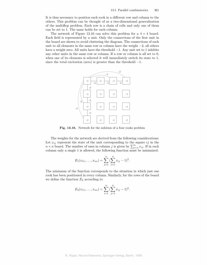
It is thus necessary to position each rook in a different row and column to theothers. This problem can be thought of as a two-dimensional generalizationof the multiflop problem. Each row is a chain of cells and only one of themcan be set to 1. The same holds for each column.

The network of Figure 13.16 can solve this problem for a 4 × 4 board.Each field is represented by a unit. Only the connections of the first unit inthe board are shown to avoid cluttering the diagram. The connections of eachunit to all elements in the same row or column have the weight −2, all othershave a weight zero. All units have the threshold −1. Any unit set to 1 inhibitsany other units in the same row or column. If a row or column is all set to 0,when one of its elements is selected it will immediately switch its state to 1,since the total excitation (zero) is greater than the threshold −1.

–2–2

–2 –2 –2

–2

–2

–2

–2

–2

–1 –1 –1 –1

–1

–1

–1

–1 –1 –1

–1 –1 –1

–1 –1 –1

Fig. 13.16. Network for the solution of a four rooks problem

The weights for the network are derived from the following considerations:Let xij represent the state of the unit corresponding to the square ij in then× n board. The number of ones in column j is given by

∑ni=1 xij . If in each

column only a single 1 is allowed, the following function must be minimized:

E1(x11, . . . , xnn) =n∑

j=1

(n∑

i=1

xij − 1)2.

The minimum of the function corresponds to the situation in which just onerook has been positioned in every column. Similarly, for the rows of the boardwe define the function E2 according to

E2(x11, . . . , xnn) =n∑

i=1

(n∑

j=1

xij − 1)2.




We want to minimize the function E = E1 + E2. The general strategy is toreduce its analytical expression to a Hopfield form. The necessary algebraicsteps can be avoided by noticing that the expression for E1 is the sum of nindependent functions (one per column). The term (

∑ni=1 xij−1)2 corresponds

to a multiflop problem. The weights for the edges in each column can be setto −2, as was done before in the multiflop problem. The same is done for eachrow: the weights between any unit and its row partners are set to −2. Only thethresholds must be selected with a little more care. The simple juxtapositionof a row-multiflop with a column-multiflop at each field will give us a thresholdof −1 + (−1) = −2. This would mean that each row or column can containup to two elements whose state is 1. This is avoided by setting the thresholdsof the units to −1. The resulting network is the one shown in Figure 13.16.Each field will be forced to adopt the state zero whenever another unit is setto 1 in its own row or its own column.

13.5.4 The eight queens problem

The well-known eight queens problem can also be solved with a Hopfield net-work. It is just a generalization of the rooks problem, since now the diagonalsof the board will also be considered. Each diagonal can be occupied at mostonce by a queen. As before with the rooks problem, we solve this task byoverlapping multiflop problems at each square. Figure 13.17 shows how threemultiflop chains have to be considered for each field. The diagram shows a4×4 board and the overlapping of multiflop problems for the upper left squareon the board. This overlapping provides us with the necessary weights, whichare set to wij = −2, when unit i is different from unit j and belongs to thesame row, column or diagonal as unit j. Otherwise we set wij to zero. Thethresholds of all units are set to −1.

Fig. 13.17. The eight queens problem

A computer simulation shows, however, that this simple connection pat-tern does not always provide a correct solution for the n-queens problem. The




proposed connection weights produce an energy function in which local min-ima with less than n queens are possible. The only alternative if such a stablestate is found is to start the simulation again.

It is not possible to set the weights of the network of Figure 13.17 in such away as to obtain only correct solutions. The difficulty is that diagonals can beoccupied by a queen but they can also be unoccupied. Simple overlapping ofmultiflop problems does not work any more. The energy function has becomemuch more complex than in the previous cases and we now have to achievecompromises between the weights which we choose for rows and columns andfor diagonals.

13.5.5 The traveling salesman

The Traveling Salesman Problem (TSP) is one of the most celebrated bench-marks in combinatorics. It is simple to state and visualize and it is NP-complete. If we can solve the TSP efficiently, we can provide an efficientsolution for other problems in the class NP. Hopfield and Tank [200] werethe first to try to solve the TSP using a neural network.

A

BC

D

E

F

G

Fig. 13.18. A TSP and its solution

In the TSP we are looking for a path through n cities S1, S2, . . . , Sn, suchthat every city is visited at least once and the length of a round trip is minimal.Let dij denote the distance between the cities Si and Sj . A round trip canbe represented using a matrix. Each of the n rows of the matrix is associatedwith a city. The columns are labeled 1 through n and they correspond to then necessary visits. The following matrix shows a path going through the citiesS1, S2, S3 and S4 in that same order:




1 2 3 4S1 1 0 0 0S2 0 1 0 0S3 0 0 1 0S4 0 0 0 1

A single 1 is allowed in each row and each column, otherwise the salesmanwould visit a city twice or two cities simultaneously. This matrix must fulfillthe same conditions as in the rooks problem and we can again use a networkin which a unit is used to represent each entry in the matrix (the new “chessboard”).

Solving the TSP requires minimizing the length of the round trip, that isof

L =12

n∑i,j,k

dijxikxj,k+1,

where xik represents the state of the unit corresponding to the entry ik inthe matrix. When xik and xj,k+1 are both 1, this means that the city Si isvisited in the k-th step and the city Sj in the step k+1. The distance betweenboth cities must be added to the total length of the round trip. We use theconvention that the column n+ 1 is equal to the first column of the matrix,so that we always obtain a round trip.

In the minimization problems we must include the constraints for a validround trip. It is necessary to add the energy function of the rooks problem tothe length L to obtain the new energy function E, which is given by

E =12

n∑i,j,k

dijxikxj,k+1 +γ

2(

n∑j=1

(n∑

i=1

xij − 1)2 +n∑

i=1

(n∑

j=1

xij − 1)2),

where the constant γ regulates how much weight is given to the minimizationof the length or to the generation of legal paths. The first summation to theright of the equal sign already has the form of a Hopfield energy function; theexpression in parentheses has it too, since it is the energy function of a rooksproblem. The weights for the network can be deduced immediately from thisexpression: the weights of edges between units in the same row or columnmust be set to −γ and the thresholds of the units to −γ/2. The weights mustbe modified by including the length between states, so that the weight of theedge between unit ik and unit j, k + 1 becomes

wik,jk+1 = −dij + tik,jk+1

where tik,jk+1 = −γ whenever the units belong to the same row or column,otherwise tik,jk+1 is zero.

With this network we can try to find solutions of the TSP. A simulationshows that the generated routes are sometimes not legal, because one city isnot visited or more than one city is visited in a single step. We can always




force the network to generate legal tours: it is only necessary to set γ to avery large value so as to obliterate the contribution of the cities’ distances. Ifγ is zero, we do not care whether the tour is a legal one and only the totallength is minimized (by choosing an “empty” tour). Since the value of γ isnot prescribed, it can be found by trial and error. In general the networkwill not be capable of finding the global minimum and because large TSPs(with more than 100 cities) have so many local minima, it is difficult to decidewhether the local minimum that has been found is a good approximation tothe optimal result. The whole approach is dependent on the existence of real,massively parallel systems, since the number of units required to solve a TSPincreases quadratically with the number n of cities (and the number of weightsincreases proportionally to n4).

13.5.6 The limits of Hopfield networks

The first articles of Hopfield and Tank on parallel solutions to combinatorialproblems received a lot of attention [200, 201]. The theoretical question waswhether this could be a method to solve NP-hard problems or at least to getan approximate solution in polynomial time. In the following years many otherresearchers tried to extend the range of combinatorial problems that could besolved using Hopfield’s technique, trying to improve the quality of the resultsat the same time. It emerged that well-behaved average problems could besolved efficiently. However, these average results should be compared to theexpected running time for the worst case. Bruck and Goodman [74] showedthat a polynomially bounded network (on the size of the problem) is unableto find the global minimum of the energy function of NP-complete problems(encoded as Hopfield networks) with a 100% guarantee. Stated in anotherway: if we try to transform all local minima of the Hopfield network into anoptimal solution of the combinatorial problem, the size of the network explodesexponentially. We proceed to prove the result of Bruck and Goodman, but wemust first introduce an additional complexity class: the complement of theclass NP.

The class NP of nondeterministic problems solvable in polynomial time isdifferent from the class P of problems solvable in polynomial time not only inthe way exposed already in Chap. 10. If a problem is a member of the classP , the same is true for the complementary problem. The complement of thedecision problem “For the problem instance I, is X true for I?”is just “Forthe problem instance I, is X false for I?”. A deterministic polynomial timealgorithm terminates on each of the two questions. It is only necessary tosubstitute “true” for “false” to transform a polynomial time algorithm for aproblem in P in an algorithm for its complement. But this is not necessarily sofor problems in NP. A solution for the Traveling Salesman Decision Problem(TSDP), that is, the computation of the tour’s length and the comparisonwith the decision’s threshold, can be verified in polynomial time. However,the complementary problem has the wording “Is there no tour with a total




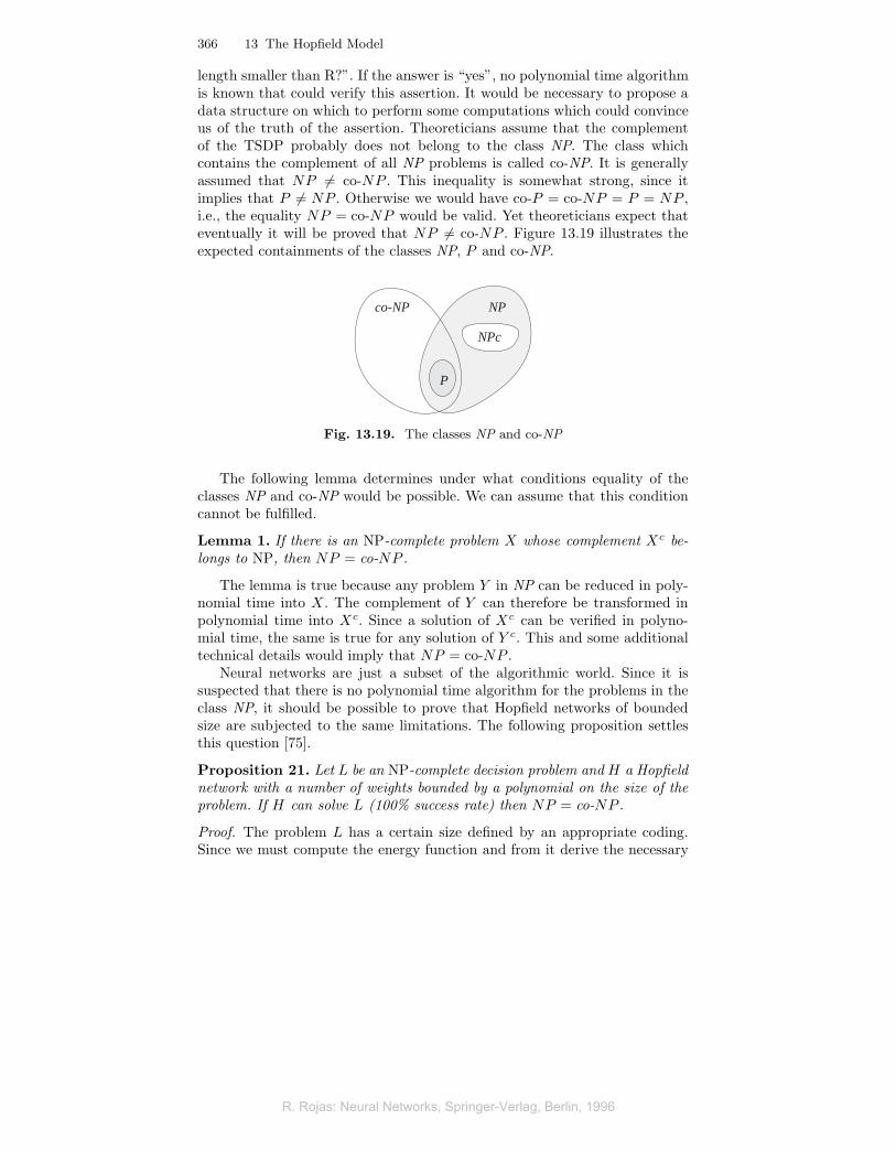
length smaller than R?”. If the answer is “yes”, no polynomial time algorithmis known that could verify this assertion. It would be necessary to propose adata structure on which to perform some computations which could convinceus of the truth of the assertion. Theoreticians assume that the complementof the TSDP probably does not belong to the class NP. The class whichcontains the complement of all NP problems is called co-NP. It is generallyassumed that NP �= co-NP . This inequality is somewhat strong, since itimplies that P �= NP . Otherwise we would have co-P = co-NP = P = NP ,i.e., the equality NP = co-NP would be valid. Yet theoreticians expect thateventually it will be proved that NP �= co-NP . Figure 13.19 illustrates theexpected containments of the classes NP, P and co-NP.

NPco-NP

P

NPc

Fig. 13.19. The classes NP and co-NP

The following lemma determines under what conditions equality of theclasses NP and co-NP would be possible. We can assume that this conditioncannot be fulfilled.

Lemma 1. If there is an NP-complete problem X whose complement Xc be-longs to NP, then NP = co-NP .

The lemma is true because any problem Y in NP can be reduced in poly-nomial time into X . The complement of Y can therefore be transformed inpolynomial time into Xc. Since a solution of Xc can be verified in polyno-mial time, the same is true for any solution of Y c. This and some additionaltechnical details would imply that NP = co-NP .

Neural networks are just a subset of the algorithmic world. Since it issuspected that there is no polynomial time algorithm for the problems in theclass NP, it should be possible to prove that Hopfield networks of boundedsize are subjected to the same limitations. The following proposition settlesthis question [75].

Proposition 21. Let L be an NP-complete decision problem and H a Hopfieldnetwork with a number of weights bounded by a polynomial on the size of theproblem. If H can solve L (100% success rate) then NP = co-NP .

Proof. The problem L has a certain size defined by an appropriate coding.Since we must compute the energy function and from it derive the necessary



13.6 Implementation of Hopfield networks 367

weights for H , a polynomial bound on the total number of weights is neces-sary. A Hopfield network always finds a local minimum of its energy function.In our case, a 100% hit rate means that all local minima of the energy func-tion should make possible a decision on the truth or falsity of the decisionproblem L. The Hopfield network can be considered a data structure thatmakes possible the verification of the found solution. It is only necessary toverify whether the solution found by the network is indeed a local minimumof the energy function. The polynomial size of the net makes this verificationpossible in polynomial time. The decision problem and the complement are,in this case, completely symmetric. The TSDP can be answered with “yes” ifthe tour found by the network is shorter than the decision threshold. But thecomplement of the TSDP can be decided also just by comparing the lengthof the optimal tour found with the decision threshold. Therefore the comple-ment of L is a member of the class NP and it follows from Lemma 1 thatNP = co-NP . Since it is generally assumed that this cannot be so, thereshould be a contradiction in the premises. The network H does not existunless NP = co-NP . �

Even if we content ourselves with a polynomially bounded network thatcan provide approximate solutions (for example, TSP round-trips not larger bya given ε than the optimal tour), no such network can be built. It is because ofthis inherent limitation that some authors have sought to introduce stochasticfactors into the networks, as we will discuss when we deal with Boltzmannmachines in the next chapter.

13.6 Implementation of Hopfield networks

Hopfield networks as massively parallel systems are only interesting if theycan be implemented in hardware and not just simulated in a sequential com-puter. Some proposals have been made for special chips capable of simulatingHopfield networks but the most promising approach are optical computers,capable of solving the connectivity problem of neural networks.

13.6.1 Electrical implementation

In 1984 Hopfield proposed an electrical realization of his model which usesa circuit very similar to the ones used by Steinbuch (Chap. 18) [199]. Fig-ure 13.20 shows a diagram of the circuit. The outputs of the amplifiersx1, x2, . . . , xn are interpreted as the states of the Hopfield units. Their com-plements ¬x1,¬x2, . . . ,¬xn are produced by inverters. All states and theircomplements are fed back to the input of the electrical circuit. An electricalcontact is represented by a small circle. A resistance is present at each con-tact point. The connection r13, for example, contains a resistor with resistancer13 = 1/w13. The constants wij represent the weights of the Hopfield network




between the units i and j. Inhibiting connections between one unit and an-other (that is, connections with negative weights) are simulated by connectingone inverted output of a unit to the other one. In Figure 13.20, for example,the connection points in the upper row all come from the inverted output ofunit 1.

...x1

1

2

2

3 3

r13

x x

x x

x

Fig. 13.20. Electrical implementation of a Hopfield network

In a network with n amplifiers the current Ii at the input to the i-thamplifier is given by

Ii =n∑

j=1

xj

rij=

n∑j=1

xjwij ,

where we have used the convention that rij is negative if the inverted valueof xj has been connected to the input of the amplifier xi. The current Ii rep-resents the excitation of unit i. The amplifier transforms the total excitationinto 0 or 1 according to a certain electrical threshold, which can be set to anarbitrary positive value.

This simple circuit can be used to simulate Hopfield networks in a fractionof the time needed by a sequential computer. If the circuit is provided withvariable resistors it is then possible to implement some learning algorithmsdirectly in hardware.

13.6.2 Optical implementation

The most important computation that must be accelerated for a fast simula-tion of Hopfield networks is the vector matrix multiplication. Computation ofthe excitation of a node requires such an operation every time a unit’s stateis to be updated. Optical methods can be used to perform this numerical op-eration faster. Figure 13.21 shows an optical realization of the Hopfield model[132].



13.6 Implementation of Hopfield networks 369

The logical structure is in principle the same as in the network of Fig-ure 13.20, but the vector matrix multiplication is computed analogically usingoptical techniques. The n binary values which represent the network’s stateare projected through the vertical lens to the left of the arrangement. Thelens projects each value xi onto the corresponding row of an optical mask.Each row i in the mask is divided into fields which represent the n weightswi1, wi2, . . . , win. Each field is partially darkened according to the value ofthe corresponding weight. The individual unit states are projected using lightemitting diodes and the luminosity is proportional to the corresponding xi

value. The light going through the mask is collected by another lens in sucha way that all the incoming light from a column is collected at a single posi-tion. The amount of light that goes through the mask is proportional to theproduct of xi and wij at each position ij of the mask. The incoming light atthe j-th detector represents the total excitation of unit j, which is equal to

sj =n∑

i=1

wijxi.

The total excitation of the unit j can now be processed by an analog or digitalcircuit to produce the unit state which is used again in a new iteration of thenetwork.

wx

illuminated row

input fromlight emittingdiodes ij

i

excitationof the j-th unit

SLM mask

lens

lens

Fig. 13.21. Optical implementation of a Hopfield network

The difference compared with the electrical model is that the weights andsignals must be normalized and scaled to fit the kind of optical processingbeing done. The most significant difference is the absence of direct connections.The light paths do not affect each other, so that it is possible to implementmuch larger networks than in the purely electrical realization. We will comeback to the topic of optical implementations when we discuss neural hardwarein Chap. 18.




13.7 Historical and bibliographical remarks

With the introduction in 1982 of the model named after him, John Hopfieldestablished the connection between neural networks and physical systems ofthe type considered in statistical mechanics. This in turn gave computer sci-entists a whole new arsenal of mathematical tools for the analysis of neuralnetworks. Other researchers had already considered more general associativememory models in the 1970s, but by restricting the architecture of the net-work to a symmetric connection matrix with a zero diagonal, it was possibleto design recurrent networks with stable states. With the introduction of theconcept of the energy function, the convergence properties of the networkscould be more easily analyzed.

The Hopfield network also has the advantage, in comparison with othermodels, of a simple technical implementation using electronic or optical de-vices [132]. The computing strategy used when updating the network statescorresponds to the relaxation methods traditionally used in physics [92].

The properties of Hopfield networks have been investigated since 1982 us-ing the theoretical tools of statistical mechanics [322]. Gardner [155] publisheda classical treatise on the capacity of the perceptron and its relation to theHopfield model. The total field sensed by particles with a spin can be com-puted using the methods of mean field theory. This simplifies a computationwhich is hopeless without the help of some statistical assumptions [189]. Usingthese methods Amit et al. [24] showed that the number of stable states in aHopfield network of n units is bounded by 0.14n. A recall error is toleratedonly 5% of the time. This upper bound is one of the most cited numbers inthe theory of Hopfield networks.

In 1988 Kosko proposed the BAM model, which is a kind of “missinglink” between conventional associative memories and Hopfield networks. Manyother variations have been proposed since, some of them with asynchronous,others with synchronous dynamics [231]. Hopfield networks have also beenstudied from the point of view of dynamical systems. In this respect spinglass models play a relevant role. These are materials composed of particleswith a spin and mutual interactions [412].

Combinatorial problems have a long tradition, but a really systematictheory capable of unifying the myriad of heuristic methods developed in thepast was first developed in the 1960s and 1970s [361]. The important pointwas the increasingly important role played by computers and the emergenceof a new attitude which tried to reach whole classes of problems and notjust individual cases. An important research theme which remains is how tosplit a combinatorial problem into subtasks that can be assigned to differentprocessors [160].

The efforts of Hopfield and Tank with the TSP led to many other similarexperiments in related fields. Wilson and Pawley [456] repeated their experi-ments but they could not confirm the optimistic results of the former authors.The main difficulty is that complex combinatorial problems produce an expo-



13.7 Historical and bibliographical remarks 371

nential number of local minima of the energy function. In sequential comput-ers, Hopfield models cannot compete with conventional methods [224]. Manyheuristics have been proposed for the TSP, starting with the classical work byKernighan and Lin [274]. The only way to make Hopfield models competitiveis through the use of special hardware. Sheu et al. have obtained interestingresults and significant speedup in comparison with sequential computers byusing a technique they call hardware annealing.

One of the first to deal with the intrinsic limits of the Hopfield model forthe solution of the TSP was Abu-Mostafa [3], who nevertheless consideredonly the case of networks of constant size. Bruck and Goodman [75] consid-ered networks of variable but polynomially bounded size and obtained thesame negative results. Although this almost meant the “death of the travel-ing salesman” [322], the Hopfield model and its stochastic variants have beenapplied in many other fields, such as psychology, simulation of ensembles ofbiological neural networks, and chaotic behavior of neural circuits.

The optical implementation of Hopfield networks is a promising field ofresearch. Other than masks, holograms can also be used to store the networkweights [352]. The main technical problem is still the size reduction of the op-tical components, which could make them a viable alternative to conventionalelectronic systems.

Exercises

1. Train a Hopfield network in the computer using the perceptron learningalgorithm.

2. Solve a TSP of 10 cities with a Hopfield network. How many weights doyou need for the network?

3. Compute the energy of the different possible states of the network shownin Figure 13.6. Do the same for Figure 13.7 assigning some values to theweights and thresholds.





Documents

Chapter 13 of Rojas Neural Networks a Systematic Introductionpage.mi.fu-berlin.de/rojas/neural/chapter/K13.pdf · state update. We adopt the additional simpliﬁcation that the state