18 Hardware for Neural Networks - UserPages < Tec < …page.mi.fu-berlin.de/rojas/neural/chapter/K18.pdfR. Rojas: Neural Networks, Springer-Verlag, Berlin, 1996 452 18 Hardware for

18

Hardware for Neural Networks

18.1 Taxonomy of neural hardware

This chapter concludes our analysis of neural network models with an overviewof some hardware implementations proposed in recent years. In the first chap-ter we discussed how biological organisms process information. We are nowinterested in finding out how best to process information using electronic de-vices which in some way emulate the massive parallelism of the biologicalworld. We show that neural networks are an attractive option for engineeringapplications if the implicit parallelism they offer can be made explicit withappropriate hardware. The important point in any parallel implementationof neural networks is to restrict communication to local data exchanges. Thestructure of some of those architectures, such as systolic arrays, resemblescellular automata.

There are two fundamentally different alternatives for the implementationof neural networks: a software simulation in conventional computers or a spe-cial hardware solution capable of dramatically decreasing execution time. Asoftware simulation can be useful to develop and debug new algorithms, aswell as to benchmark them using small networks. However, if large networksare to be used, a software simulation is not enough. The problem is the timerequired for the learning process, which can increase exponentially with thesize of the network. Neural networks without learning, however, are rather un-interesting. If the weights of a network were fixed from the beginning and werenot to change, neural networks could be implemented using any programminglanguage in conventional computers. But the main objective of building spe-cial hardware is to provide a platform for efficient adaptive systems, capableof updating their parameters in the course of time. New hardware solutionsare therefore necessary [54].

R. Rojas: Neural Networks, Springer-Verlag, Berlin, 1996


452 18 Hardware for Neural Networks

18.1.1 Performance requirements

Neural networks are being used for many applications in which they are moreeffective than conventional methods, or at least equally so. They have beenintroduced in the fields of computer vision, robot kinematics, pattern recogni-tion, signal processing, speech recognition, data compression, statistical anal-ysis, and function optimization. Yet the first and most relevant issue to bedecided before we develop physical implementations is the size and computingpower required for the networks.

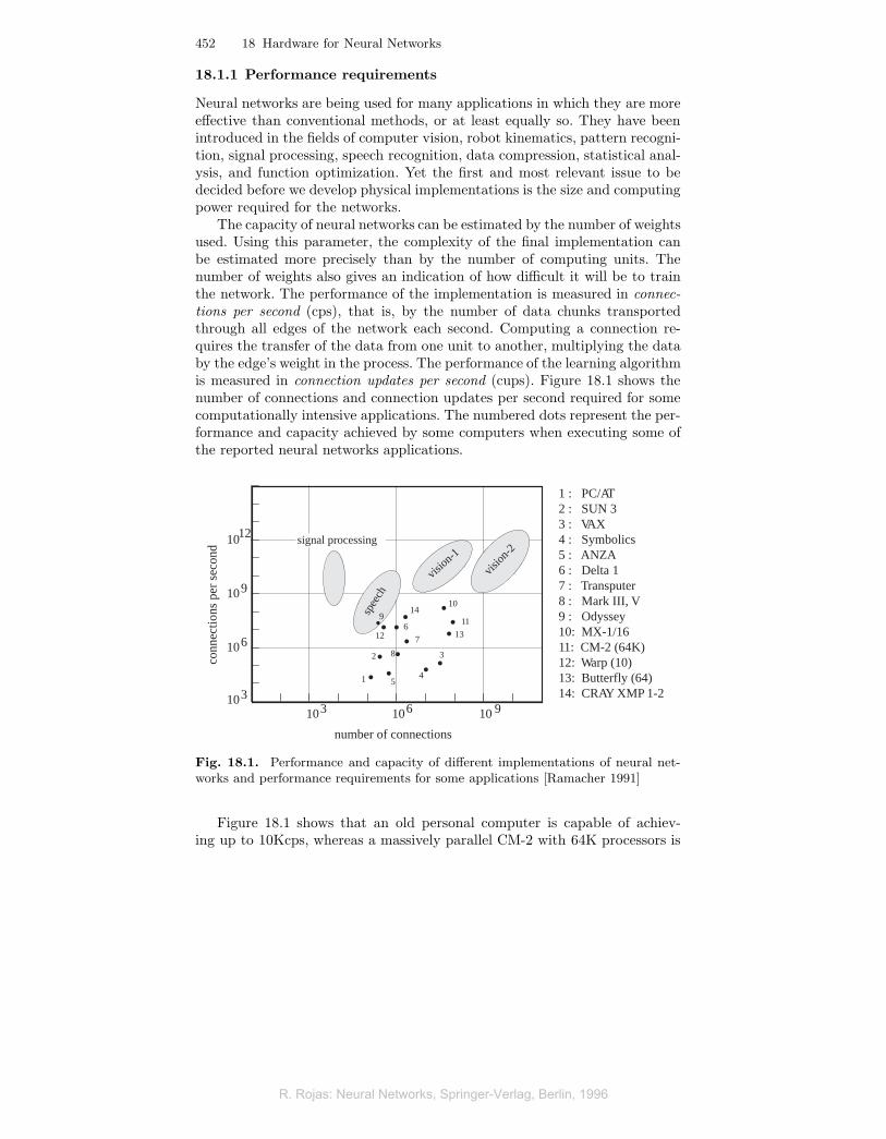
The capacity of neural networks can be estimated by the number of weightsused. Using this parameter, the complexity of the final implementation canbe estimated more precisely than by the number of computing units. Thenumber of weights also gives an indication of how difficult it will be to trainthe network. The performance of the implementation is measured in connec-tions per second (cps), that is, by the number of data chunks transportedthrough all edges of the network each second. Computing a connection re-quires the transfer of the data from one unit to another, multiplying the databy the edge’s weight in the process. The performance of the learning algorithmis measured in connection updates per second (cups). Figure 18.1 shows thenumber of connections and connection updates per second required for somecomputationally intensive applications. The numbered dots represent the per-formance and capacity achieved by some computers when executing some ofthe reported neural networks applications.

1

2

5

8

4

3

13

11

1014

6

712

9spee

ch

vision

-1

vision

-2signal processing

10 10 103 6 9

number of connections

conn

ectio

ns p

er s

econ

d

10

10

10

1012

9

6

3

1 : PC/AT2 : SUN 33 : VAX4 : Symbolics5 : ANZA6 : Delta 17 : Transputer8 : Mark III, V9 : Odyssey10: MX-1/1611: CM-2 (64K)12: Warp (10)13: Butterfly (64)14: CRAY XMP 1-2

•••

••

••

••

••

•

••

Fig. 18.1. Performance and capacity of different implementations of neural net-works and performance requirements for some applications [Ramacher 1991]

Figure 18.1 shows that an old personal computer is capable of achiev-ing up to 10Kcps, whereas a massively parallel CM-2 with 64K processors is



18.1 Taxonomy of neural hardware 453

capable of providing up to 10 Mcps of computing power. With such perfor-mance we can deal with speech recognition in its simpler form, but not withcomplex computer vision problems or more sophisticated speech recognitionmodels. The performance necessary for this kind of application is of the orderof Giga-cps. Conventional computers cannot offer such computing power withan affordable price-performance ratio. Neural network applications in whicha person interacts with a computer require compact solutions, and this hasbeen the motivation behind the development of many special coprocessors.Some of them are listed in Figure 18.1, such as the Mark III or ANZA boards[409].

A pure software solution is therefore not viable, yet it remains openwhether an analog or a digital solution should be preferred. The next sec-tions deal with this issue and discuss some of the systems that have beenbuilt, both in the analog and the digital world.

18.1.2 Types of neurocomputers

To begin with, we can classify the kinds of hardware solution that have beenproposed by adopting a simple taxonomy of hardware models. This will sim-plify the discussion and help to get a deeper insight into the properties ofeach device. Defining a taxonomy of neurocomputers requires considerationof three important factors:

• the kind of signals used in the network,• the implementation of the weights,• the integration and output functions of the units.

The signals transmitted through the network can be coded using an analog or adigital model. In the analog approach, a signal is represented by the magnitudeof a current, or a voltage difference. In the digital approach, discrete values arestored and transmitted. If the signals are represented by currents or voltages,it is straightforward to implement the weights using resistances or transistorswith a linear response function for a certain range of values. In the case of adigital implementation, each transmission through one of the network’s edgesrequires a digital multiplication.

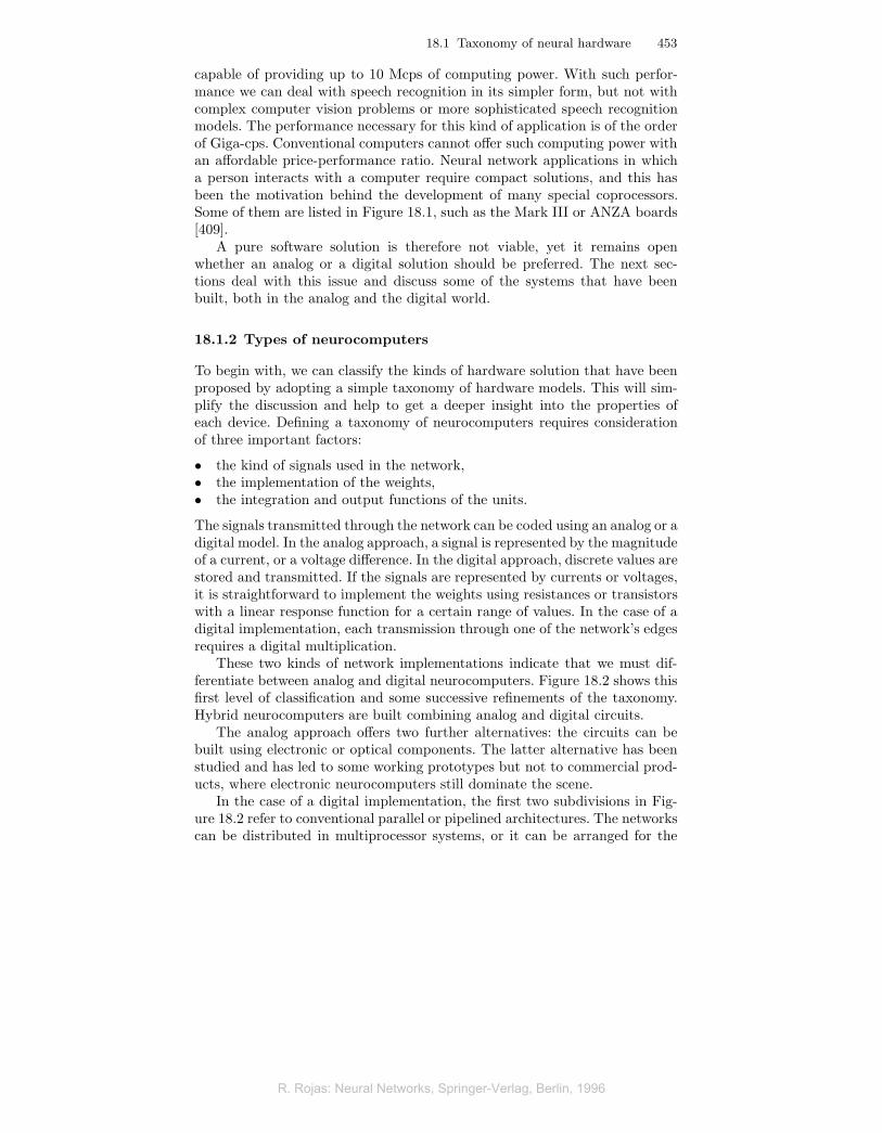
These two kinds of network implementations indicate that we must dif-ferentiate between analog and digital neurocomputers. Figure 18.2 shows thisfirst level of classification and some successive refinements of the taxonomy.Hybrid neurocomputers are built combining analog and digital circuits.

The analog approach offers two further alternatives: the circuits can bebuilt using electronic or optical components. The latter alternative has beenstudied and has led to some working prototypes but not to commercial prod-ucts, where electronic neurocomputers still dominate the scene.

In the case of a digital implementation, the first two subdivisions in Fig-ure 18.2 refer to conventional parallel or pipelined architectures. The networkscan be distributed in multiprocessor systems, or it can be arranged for the




Analog

Digital

von-Neumann multiprocessor

Vector processors

Systolic arrays

ring

2d-grid

torus

Special designs

electronic components

optical components

superscalar

SIMD

Fig. 18.2. Taxonomy of neurosystems

training set to be allocated so that each processor works with a fraction ofthe data. Neural networks can be efficiently implemented in vector processors,since most of the necessary operations are computations with matrices. Vectorprocessors have been optimized for exactly such operations.

A third digital model is that of systolic arrays. They consist of regulararrays of processing units, which communicate only with their immediateneighbors. Input and output takes place at the boundaries of the array [207].They were proposed to perform faster matrix-matrix multiplications, the kindof operation in which we are also interested for multilayered networks.

The fourth and last type of digital system consists of special chips of thesuperscalar type or systems containing many identical processors to be usedin a SIMD (single instruction, multiple data) fashion. This means that allprocessors execute the same instruction but on different parts of the data.

Analog systems can offer a higher implementation density on silicon andrequire less power. But digital systems offer greater precision, programmingflexibility, and the possibility of working with virtual networks, that is, net-works which are not physically mapped to the hardware, making it possibleto deal with more units. The hardware is loaded successively with differentportions of the virtual network, or, if the networks are small, several networkscan be processed simultaneously using some kind of multitasking.



18.2 Analog neural networks 455

18.2 Analog neural networks

In the analog implementation of neural networks a coding method is used inwhich signals are represented by currents or voltages. This allows us to thinkof these systems as operating with real numbers during the neural networksimulation.

18.2.1 Coding

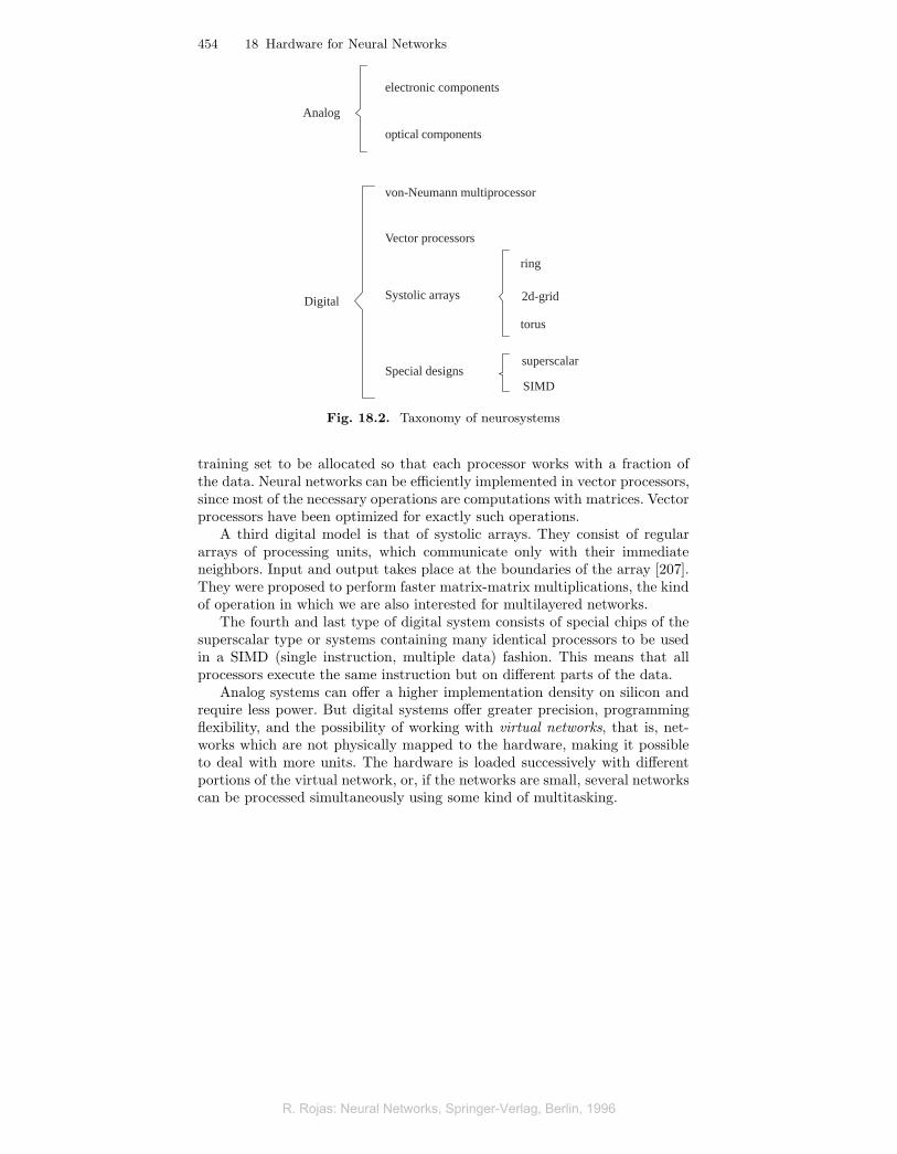
When signals are represented by currents, it is easy to compute their addi-tion. It is only necessary to make them meet at a common point. One ofthe Kirchhoff laws states that the sum of all currents meeting at a point iszero (outgoing currents are assigned a negative sign). The simple circuit ofFigure 18.3 can be used to add I1 and I2, and the result is the current I3.

I

I I

1

2 3

Fig. 18.3. Addition of electric current

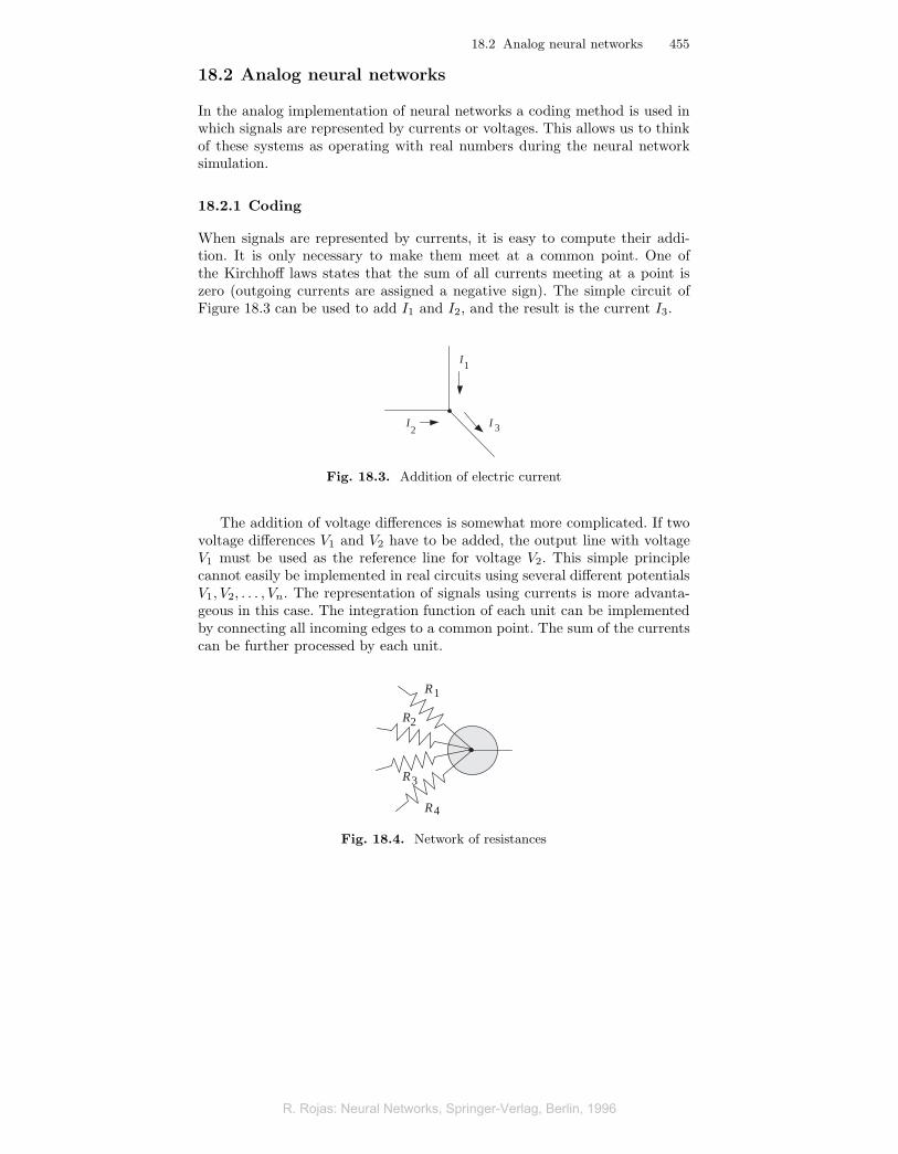
The addition of voltage differences is somewhat more complicated. If twovoltage differences V1 and V2 have to be added, the output line with voltageV1 must be used as the reference line for voltage V2. This simple principlecannot easily be implemented in real circuits using several different potentialsV1, V2, . . . , Vn. The representation of signals using currents is more advanta-geous in this case. The integration function of each unit can be implementedby connecting all incoming edges to a common point. The sum of the currentscan be further processed by each unit.

R

R

R

R

1

2

3

4

Fig. 18.4. Network of resistances




The weighting of the signal can be implemented using variable resistances.Rosenblatt used this approach in his first perceptron designs [185]. If theresistance is R and the current I, the potential difference V is given by Ohm’slaw V = RI. A network of resistances can simulate the necessary networkconnections and the resistors are the adaptive weights we need for learning(Figure 18.4).

Several analog designs for neural networks were developed in the 1970sand 1980s. Carver Mead’s group at Caltech has studied different alternativeswith which the size of the network and power consumption can be minimized[303]. In Mead’s designs transistors play a privileged role, especially for therealization of so-called transconductance amplifiers. Some of the chips devel-oped by Mead have become familiar names, like the silicon retina and thesilicon cochlea.

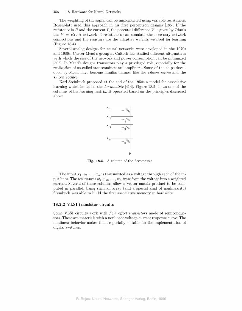
Karl Steinbuch proposed at the end of the 1950s a model for associativelearning which he called the Lernmatrix [414]. Figure 18.5 shows one of thecolumns of his learning matrix. It operated based on the principles discussedabove.

...

x

x

x

x

1

2

3

n

w 1

w

w

w

2

3

n

F

Fig. 18.5. A column of the Lernmatrix

The input x1, x2, . . . , xn is transmitted as a voltage through each of the in-put lines. The resistances w1, w2, . . . , wn transform the voltage into a weightedcurrent. Several of these columns allow a vector-matrix product to be com-puted in parallel. Using such an array (and a special kind of nonlinearity)Steinbuch was able to build the first associative memory in hardware.

18.2.2 VLSI transistor circuits

Some VLSI circuits work with field effect transistors made of semiconduc-tors. These are materials with a nonlinear voltage-current response curve. Thenonlinear behavior makes them especially suitable for the implementation ofdigital switches.




source

control electrode

sink

n + n+

isolating layer

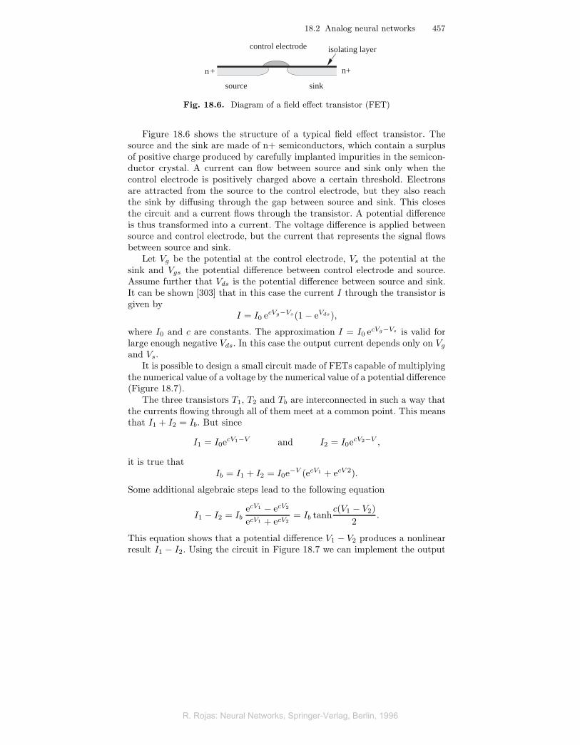
Fig. 18.6. Diagram of a field effect transistor (FET)

Figure 18.6 shows the structure of a typical field effect transistor. Thesource and the sink are made of n+ semiconductors, which contain a surplusof positive charge produced by carefully implanted impurities in the semicon-ductor crystal. A current can flow between source and sink only when thecontrol electrode is positively charged above a certain threshold. Electronsare attracted from the source to the control electrode, but they also reachthe sink by diffusing through the gap between source and sink. This closesthe circuit and a current flows through the transistor. A potential differenceis thus transformed into a current. The voltage difference is applied betweensource and control electrode, but the current that represents the signal flowsbetween source and sink.

Let Vg be the potential at the control electrode, Vs the potential at thesink and Vgs the potential difference between control electrode and source.Assume further that Vds is the potential difference between source and sink.It can be shown [303] that in this case the current I through the transistor isgiven by

I = I0 ecVg−Vs(1− eVds),

where I0 and c are constants. The approximation I = I0 ecVg−Vs is valid forlarge enough negative Vds. In this case the output current depends only on Vg

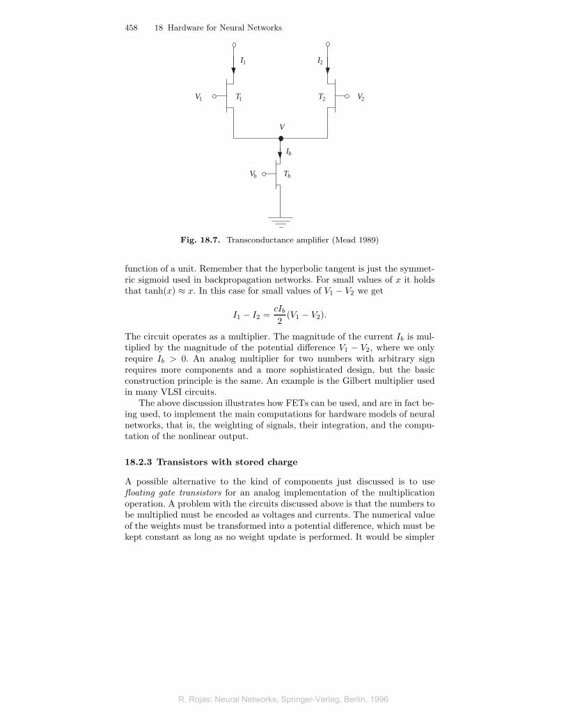
and Vs.It is possible to design a small circuit made of FETs capable of multiplying

the numerical value of a voltage by the numerical value of a potential difference(Figure 18.7).

The three transistors T1, T2 and Tb are interconnected in such a way thatthe currents flowing through all of them meet at a common point. This meansthat I1 + I2 = Ib. But since

I1 = I0ecV1−V and I2 = I0ecV2−V ,

it is true thatIb = I1 + I2 = I0e−V (ecV1 + ecV 2).

Some additional algebraic steps lead to the following equation

I1 − I2 = IbecV1 − ecV2

ecV1 + ecV2= Ib tanh

c(V1 − V2)2

.

This equation shows that a potential difference V1 − V2 produces a nonlinearresult I1 − I2. Using the circuit in Figure 18.7 we can implement the output




V

I1 I2

T1 T2V1 V2

Ib

TbVb

Fig. 18.7. Transconductance amplifier (Mead 1989)

function of a unit. Remember that the hyperbolic tangent is just the symmet-ric sigmoid used in backpropagation networks. For small values of x it holdsthat tanh(x) ≈ x. In this case for small values of V1 − V2 we get

I1 − I2 =cIb2

(V1 − V2).

The circuit operates as a multiplier. The magnitude of the current Ib is mul-tiplied by the magnitude of the potential difference V1 − V2, where we onlyrequire Ib > 0. An analog multiplier for two numbers with arbitrary signrequires more components and a more sophisticated design, but the basicconstruction principle is the same. An example is the Gilbert multiplier usedin many VLSI circuits.

The above discussion illustrates how FETs can be used, and are in fact be-ing used, to implement the main computations for hardware models of neuralnetworks, that is, the weighting of signals, their integration, and the compu-tation of the nonlinear output.

18.2.3 Transistors with stored charge

A possible alternative to the kind of components just discussed is to usefloating gate transistors for an analog implementation of the multiplicationoperation. A problem with the circuits discussed above is that the numbers tobe multiplied must be encoded as voltages and currents. The numerical valueof the weights must be transformed into a potential difference, which must bekept constant as long as no weight update is performed. It would be simpler




to store the weights using an analog method in such a way that they could beused when needed. This is exactly what floating gate transistors can achieve.

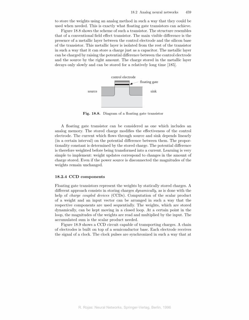
Figure 18.8 shows the scheme of such a transistor. The structure resemblesthat of a conventional field effect transistor. The main visible difference is thepresence of a metallic layer between the control electrode and the silicon baseof the transistor. This metallic layer is isolated from the rest of the transistorin such a way that it can store a charge just as a capacitor. The metallic layercan be charged by raising the potential difference between the control electrodeand the source by the right amount. The charge stored in the metallic layerdecays only slowly and can be stored for a relatively long time [185].

control electrode

sinksource

floating gate

Fig. 18.8. Diagram of a floating gate transistor

A floating gate transistor can be considered as one which includes ananalog memory. The stored charge modifies the effectiveness of the controlelectrode. The current which flows through source and sink depends linearly(in a certain interval) on the potential difference between them. The propor-tionality constant is determined by the stored charge. The potential differenceis therefore weighted before being transformed into a current. Learning is verysimple to implement: weight updates correspond to changes in the amount ofcharge stored. Even if the power source is disconnected the magnitudes of theweights remain unchanged.

18.2.4 CCD components

Floating gate transistors represent the weights by statically stored charges. Adifferent approach consists in storing charges dynamically, as is done with thehelp of charge coupled devices (CCDs). Computation of the scalar productof a weight and an input vector can be arranged in such a way that therespective components are used sequentially. The weights, which are storeddynamically, can be kept moving in a closed loop. At a certain point in theloop, the magnitudes of the weights are read and multiplied by the input. Theaccumulated sum is the scalar product needed.

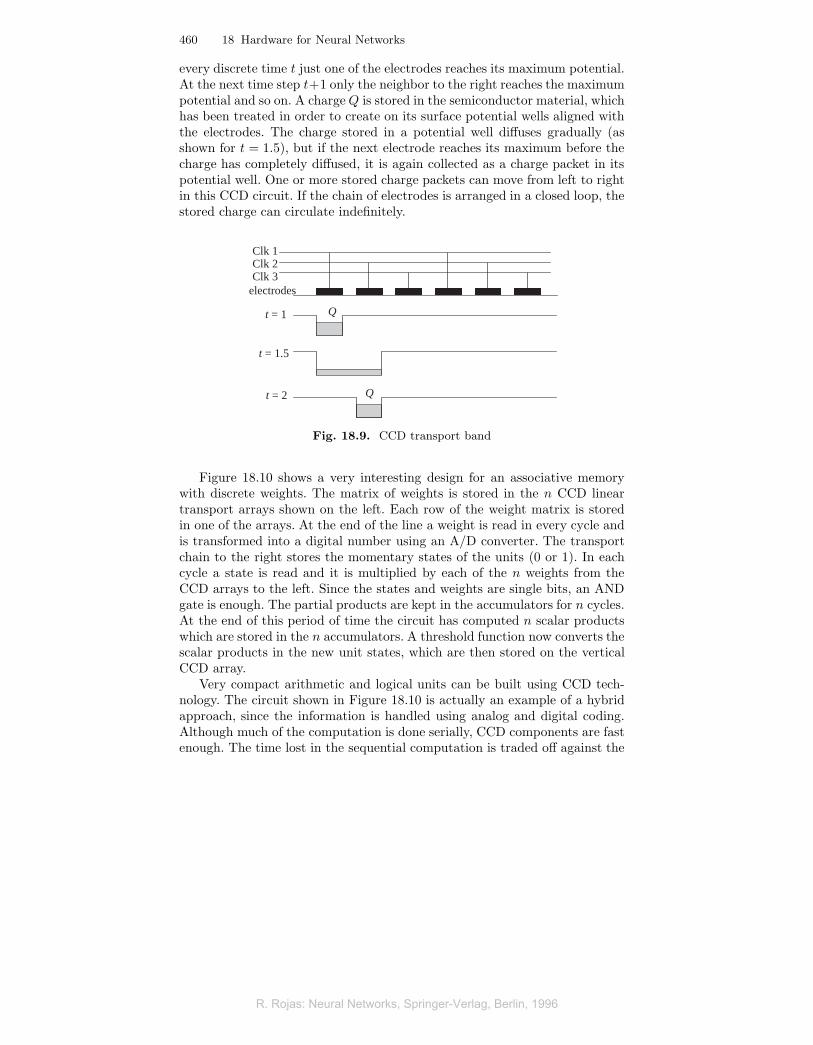
Figure 18.9 shows a CCD circuit capable of transporting charges. A chainof electrodes is built on top of a semiconductor base. Each electrode receivesthe signal of a clock. The clock pulses are synchronized in such a way that at




every discrete time t just one of the electrodes reaches its maximum potential.At the next time step t+1 only the neighbor to the right reaches the maximumpotential and so on. A chargeQ is stored in the semiconductor material, whichhas been treated in order to create on its surface potential wells aligned withthe electrodes. The charge stored in a potential well diffuses gradually (asshown for t = 1.5), but if the next electrode reaches its maximum before thecharge has completely diffused, it is again collected as a charge packet in itspotential well. One or more stored charge packets can move from left to rightin this CCD circuit. If the chain of electrodes is arranged in a closed loop, thestored charge can circulate indefinitely.

Clk 1Clk 2Clk 3

Q

Q

electrodes

t = 1.5

t = 2

t = 1

Fig. 18.9. CCD transport band

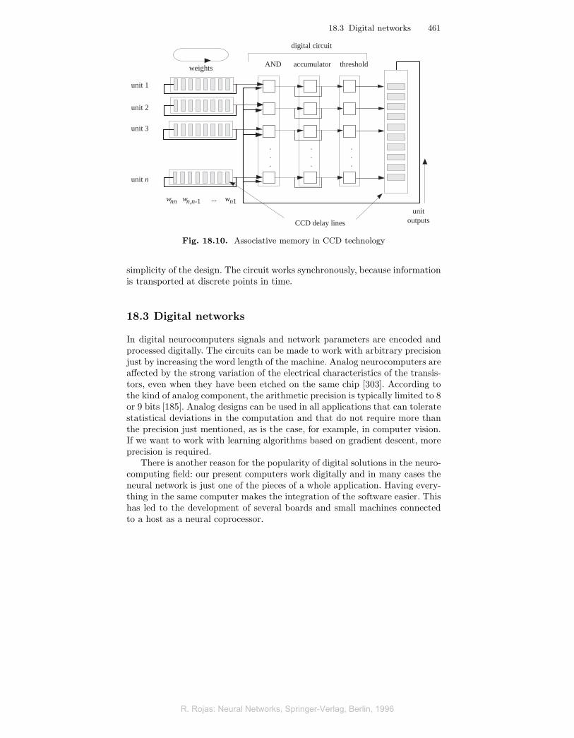
Figure 18.10 shows a very interesting design for an associative memorywith discrete weights. The matrix of weights is stored in the n CCD lineartransport arrays shown on the left. Each row of the weight matrix is storedin one of the arrays. At the end of the line a weight is read in every cycle andis transformed into a digital number using an A/D converter. The transportchain to the right stores the momentary states of the units (0 or 1). In eachcycle a state is read and it is multiplied by each of the n weights from theCCD arrays to the left. Since the states and weights are single bits, an ANDgate is enough. The partial products are kept in the accumulators for n cycles.At the end of this period of time the circuit has computed n scalar productswhich are stored in the n accumulators. A threshold function now converts thescalar products in the new unit states, which are then stored on the verticalCCD array.

Very compact arithmetic and logical units can be built using CCD tech-nology. The circuit shown in Figure 18.10 is actually an example of a hybridapproach, since the information is handled using analog and digital coding.Although much of the computation is done serially, CCD components are fastenough. The time lost in the sequential computation is traded off against the



18.3 Digital networks 461

.

.

.

.

.

.

.

.

.

weights AND accumulator threshold

digital circuit

CCD delay lines

unit 1

unit 2

unit 3

unit n

unitoutputs

w w w...nn n,n-1 n1

Fig. 18.10. Associative memory in CCD technology

simplicity of the design. The circuit works synchronously, because informationis transported at discrete points in time.

18.3 Digital networks

In digital neurocomputers signals and network parameters are encoded andprocessed digitally. The circuits can be made to work with arbitrary precisionjust by increasing the word length of the machine. Analog neurocomputers areaffected by the strong variation of the electrical characteristics of the transis-tors, even when they have been etched on the same chip [303]. According tothe kind of analog component, the arithmetic precision is typically limited to 8or 9 bits [185]. Analog designs can be used in all applications that can toleratestatistical deviations in the computation and that do not require more thanthe precision just mentioned, as is the case, for example, in computer vision.If we want to work with learning algorithms based on gradient descent, moreprecision is required.

There is another reason for the popularity of digital solutions in the neuro-computing field: our present computers work digitally and in many cases theneural network is just one of the pieces of a whole application. Having every-thing in the same computer makes the integration of the software easier. Thishas led to the development of several boards and small machines connectedto a host as a neural coprocessor.




18.3.1 Numerical representation of weights and signals

If a neural network is simulated in a digital computer, the first issue to bedecided is how many bits should be used for storage of the weights and signals.Pure software implementations use some kind of floating-point representation,such as the IEEE format, which provides very good numerical resolution at thecost of a high investment in hardware (for example for the 64-bit representa-tions). However, floating-point operations require more cycles to be computedthan their integer counterparts (unless very complex designs are used). Thishas led most neurocomputer designers to consider fixed-point representationsin which only integers are used and the position of the decimal point is man-aged by the software or simple additional circuits. If such a representationis used, the appropriate word length must be found. It must not affect theconvergence of the learning algorithms and must provide enough resolutionduring normal operation. The classification capabilities of the trained net-works depend on the length of the bit representation [223].

Some researchers have conducted series of experiments to find the appro-priate word length and have found that 16 bits are needed to represent theweights and 8 to represent the signals. This choice does not affect the con-vergence of the backpropagation algorithm [31, 197]. Based on these results,the design group at Oregon decided to build the CNAPS neurocomputer [175]using word lengths of 8 and 16 bits (see Sect. 8.2.3).

Experience with some of the neurocomputers commercially available showsthat the 8- and 16-bit representations provide enough resolution in most,but not in all cases. Furthermore, some complex learning algorithms, such asvariants of the conjugate gradient methods, require high accuracy for someof the intermediate steps and cannot be implemented using just 16 bits [341].The solution found by the commercial suppliers of neurocomputers shouldthus be interpreted as a compromise, not as the universal solution for theencoding problem in the field of neurocomputing.

18.3.2 Vector and signal processors

Almost all models of neural networks discussed in the previous chapters re-quire computation of the scalar product of a weight and an input vector.Vector and signal processors have been built with this type of application inmind and are therefore also applicable for neurocomputing.

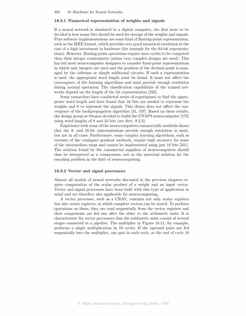
A vector processor, such as a CRAY, contains not only scalar registersbut also vector registers, in which complete vectors can be stored. To performoperations on them, they are read sequentially from the vector registers andtheir components are fed one after the other to the arithmetic units. It ischaracteristic for vector processors that the arithmetic units consist of severalstages connected in a pipeline. The multiplier in Figure 18.11, for example,performs a single multiplication in 10 cycles. If the operand pairs are fedsequentially into the multiplier, one pair in each cycle, at the end of cycle 10




one result has been computed, another at the end of cycle 11, etc. After astart time of 9 cycles a result is produced in every cycle. The partial resultscan be accumulated with an adder. After 9 + n cycles the scalar product hasbeen computed.

. . .

. . .

cycles

1011

cyclesstages

1 2 3 4 5 6 7 8 9 10x1x2xn

y1y2yn

n −1 1 0

x1y1x2y2

Fig. 18.11. Multiplier with 10 pipeline sections

The principle of vector processors has been adopted in signal processors,which always include fast pipelined multipliers and adders. A multiplicationcan be computed simultaneously with an addition. They differ from vectorprocessors in that no vector registers are available and the vectors must betransmitted from external memory modules. The bottleneck is the time neededfor each memory access, since processors have become extremely fast com-pared to RAM chips [187]. Some commercial neurocomputers are based onfast signal processors coupled to fast memory components.

18.3.3 Systolic arrays

An even greater speedup of the linear algebraic operations can be achievedwith systolic arrays. These are regular structures of VLSI units, mainly one-or two-dimensional, which can communicate only locally. Information is fed atthe boundaries of the array and is transported synchronously from one stageto the next. Kung gave these structures the name systolic arrays because oftheir similarity to the blood flow in the human heart. Systolic arrays cancompute the vector-matrix multiplication using fewer cycles than a vectorprocessor. The product of an n-dimensional vector and an n × n matrix canbe computed in 2n cycles. A vector processor would require in the order of n2

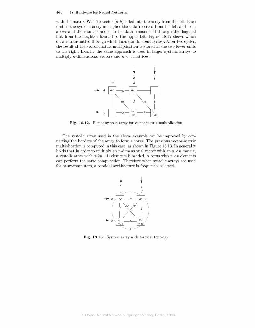
cycles for the same computation.Figure 18.12 shows an example of a two-dimensional systolic array capable

of computing a vector-matrix product. The rows of the matrix

W =(c de f

)

are used as the input from the top into the array. In the first cycle c andd constitute the input. In the second cycle e and f are fed into the array,but displaced by one unit to the right. We want to multiply the vector (a, b)




with the matrix W. The vector (a, b) is fed into the array from the left. Eachunit in the systolic array multiplies the data received from the left and fromabove and the result is added to the data transmitted through the diagonallink from the neighbor located to the upper left. Figure 18.12 shows whichdata is transmitted through which links (for different cycles). After two cycles,the result of the vector-matrix multiplication is stored in the two lower unitsto the right. Exactly the same approach is used in larger systolic arrays tomultiply n-dimensional vectors and n× n matrices.

a

b

dc

ac

b

d

e f

ae f

b

ac

bd+ac

a ae

bf+ae

Fig. 18.12. Planar systolic array for vector-matrix multiplication

The systolic array used in the above example can be improved by con-necting the borders of the array to form a torus. The previous vector-matrixmultiplication is computed in this case, as shown in Figure 18.13. In general itholds that in order to multiply an n-dimensional vector with an n×n matrix,a systolic array with n(2n−1) elements is needed. A torus with n×n elementscan perform the same computation. Therefore when systolic arrays are usedfor neurocomputers, a toroidal architecture is frequently selected.

a

b

dc

ac

b

d

ef

aef

ac

bd+ac

a ae

bf+ae

b

Fig. 18.13. Systolic array with toroidal topology




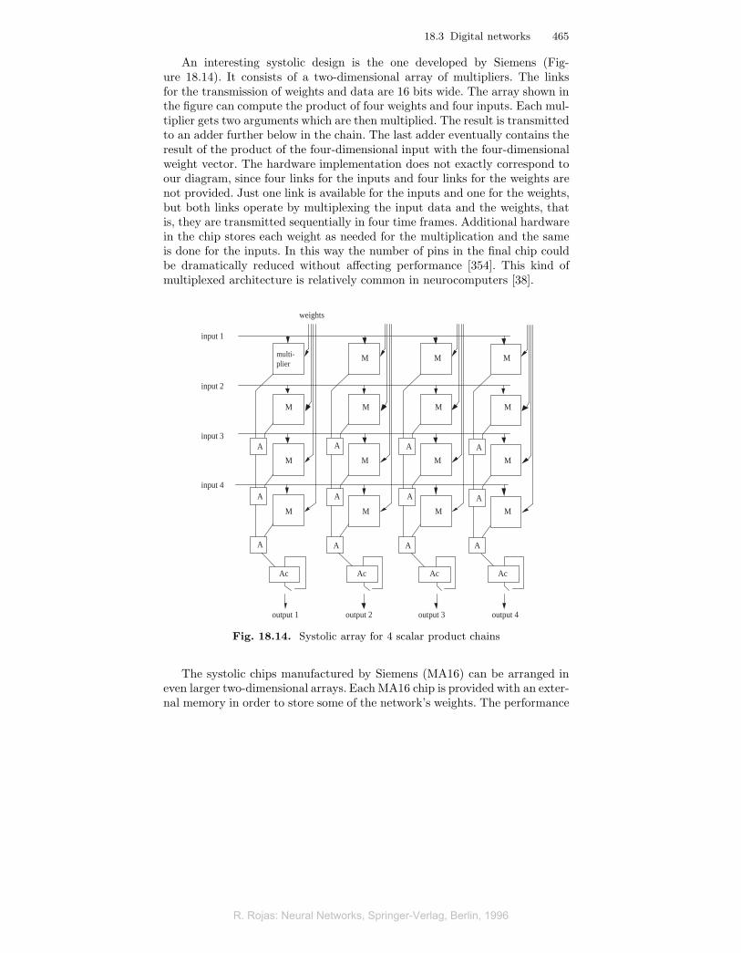
An interesting systolic design is the one developed by Siemens (Fig-ure 18.14). It consists of a two-dimensional array of multipliers. The linksfor the transmission of weights and data are 16 bits wide. The array shown inthe figure can compute the product of four weights and four inputs. Each mul-tiplier gets two arguments which are then multiplied. The result is transmittedto an adder further below in the chain. The last adder eventually contains theresult of the product of the four-dimensional input with the four-dimensionalweight vector. The hardware implementation does not exactly correspond toour diagram, since four links for the inputs and four links for the weights arenot provided. Just one link is available for the inputs and one for the weights,but both links operate by multiplexing the input data and the weights, thatis, they are transmitted sequentially in four time frames. Additional hardwarein the chip stores each weight as needed for the multiplication and the sameis done for the inputs. In this way the number of pins in the final chip couldbe dramatically reduced without affecting performance [354]. This kind ofmultiplexed architecture is relatively common in neurocomputers [38].

AcAc

multi-plier

A

A

A

A

A

A

A

A

A

A

A

M

M

M

M

M

M

M

M

M

M

M

M

M

M

M

A

weights

input 1

input 2

input 3

input 4

Ac Ac

output 1 output 2 output 3 output 4

Fig. 18.14. Systolic array for 4 scalar product chains

The systolic chips manufactured by Siemens (MA16) can be arranged ineven larger two-dimensional arrays. Each MA16 chip is provided with an exter-nal memory in order to store some of the network’s weights. The performance




promised by the creators of the MA16 should reach 128 Gcps for a 16 × 16systolic array [354]. This kind of performance could be used, for example, incomputer vision tasks. Siemens started marketing prototypes of the Synapseneurocomputer in 1995.

18.3.4 One-dimensional structures

The hardware invested in two-dimensional systolic arrays is in many casesexcessive for the vector-matrix multiplication. This is why some researchershave proposed using one-dimensional systolic arrays in order to reduce thecomplexity of the hardware without losing too much performance [438, 263].

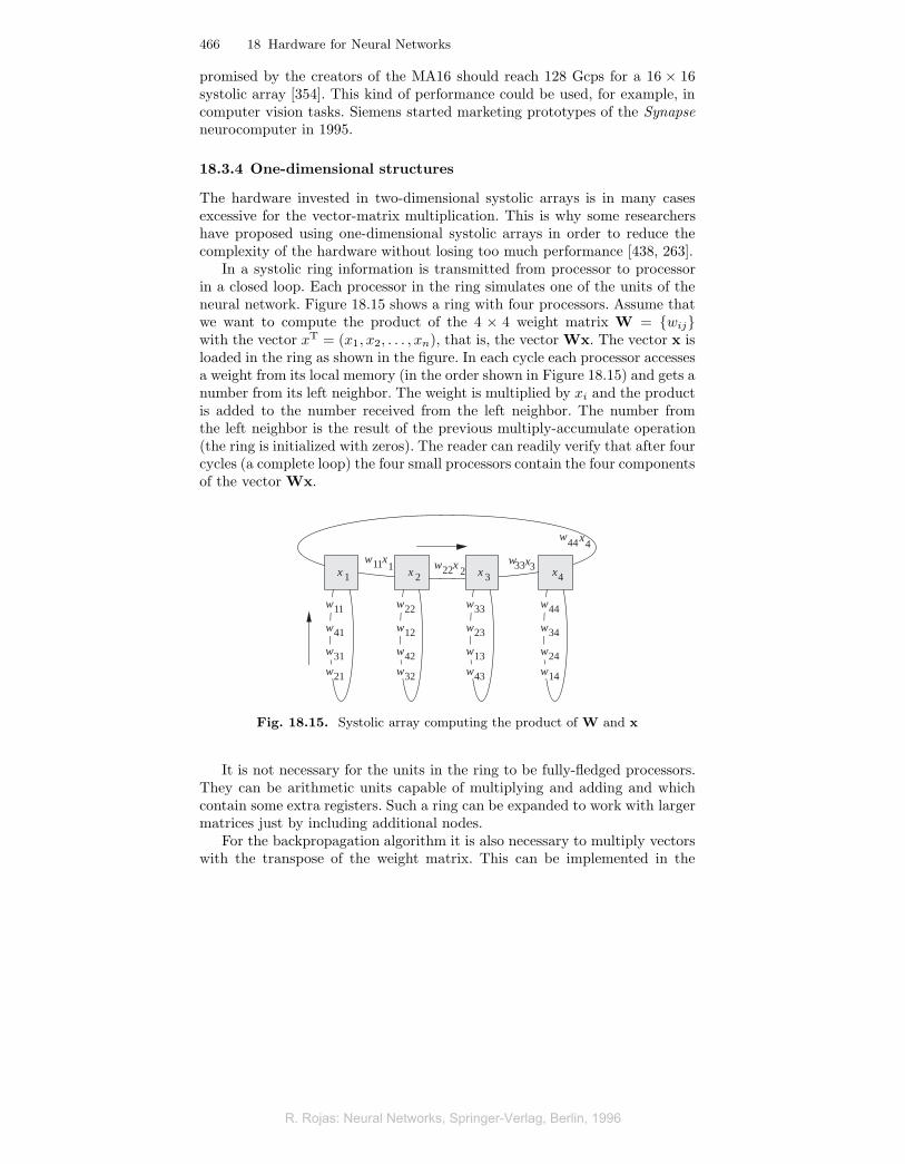
In a systolic ring information is transmitted from processor to processorin a closed loop. Each processor in the ring simulates one of the units of theneural network. Figure 18.15 shows a ring with four processors. Assume thatwe want to compute the product of the 4 × 4 weight matrix W = {wij}with the vector xT = (x1, x2, . . . , xn), that is, the vector Wx. The vector x isloaded in the ring as shown in the figure. In each cycle each processor accessesa weight from its local memory (in the order shown in Figure 18.15) and gets anumber from its left neighbor. The weight is multiplied by xi and the productis added to the number received from the left neighbor. The number fromthe left neighbor is the result of the previous multiply-accumulate operation(the ring is initialized with zeros). The reader can readily verify that after fourcycles (a complete loop) the four small processors contain the four componentsof the vector Wx.

11

w22

w12

w42

w32

w33

w23

w13

w43

w44

w34

w24

w14

w11

w41

w31

w21

x 1 x 2 x 3 x4

x1

w22x 2w 33x3w

44x4w

Fig. 18.15. Systolic array computing the product of W and x

It is not necessary for the units in the ring to be fully-fledged processors.They can be arithmetic units capable of multiplying and adding and whichcontain some extra registers. Such a ring can be expanded to work with largermatrices just by including additional nodes.

For the backpropagation algorithm it is also necessary to multiply vectorswith the transpose of the weight matrix. This can be implemented in the




w22

w12

w42

w32

w33

w23

w13

w43

w44

w34

w24

w14

w11

w41

w31

w21

x 1 x 2 x 3 x4x

1 x2

x3

x4

Fig. 18.16. Systolic array computing the product of the transpose W and x

same ring by making some changes. In each cycle the number transmitted tothe right is xi and the results of the multiplication are accumulated at eachprocessor. After four cycles the components of the product WTx are storedat each of the four units.

A similar architecture was used in the Warp machine designed by Pomer-leau and others at Princeton [347]. The performance reported was 17 Mcps.Jones et al. have studied similar systolic arrays [226].

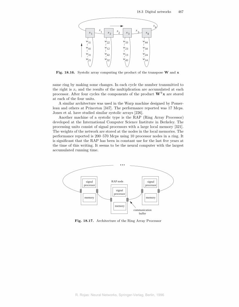
Another machine of a systolic type is the RAP (Ring Array Processor)developed at the International Computer Science Institute in Berkeley. Theprocessing units consist of signal processors with a large local memory [321].The weights of the network are stored at the nodes in the local memories. Theperformance reported is 200–570 Mcps using 10 processor nodes in a ring. Itis significant that the RAP has been in constant use for the last five years atthe time of this writing. It seems to be the neural computer with the largestaccumulated running time.

signalprocessor

memory

signalprocessor

memory

signalprocessor

memory

communicationbuffer

RAP node

...

Fig. 18.17. Architecture of the Ring Array Processor




Figure 18.17 shows the architecture of the RAP. The local memory of eachnode is used to store a row of the weight matrix W, so that each processor cancompute the scalar product of a row with the vector (x1, x2, . . . , xn)T. Theinput vector is transmitted from node to node. To compute the product WTxpartial products are transmitted from node to node in systolic fashion. Theweight updates can be made locally at each node. If the number of processorsis lower than the dimension of the vector and matrix rows, then each processorstores two or more rows of the weight matrix and computes as much as needed.The advantage of this architecture compared to a pure systolic array is thatit can be implemented using off-the-shelf components. The computing nodesof the RAP can also be used to implement many other non-neural operationsneeded in most applications.

18.4 Innovative computer architectures

The experience gained from implementations of neural networks in conven-tional von Neumann machines has led to the development of complete mi-croprocessors especially designed for neural networks applications. In somecases the SIMD computing model has been adopted, since it is relatively easyto accelerate vector-matrix multiplications significantly with a low hardwareinvestment. Many authors have studied optimal mappings of neural networkmodels onto SIMD machines [275].

18.4.1 VLSI microprocessors for neural networks

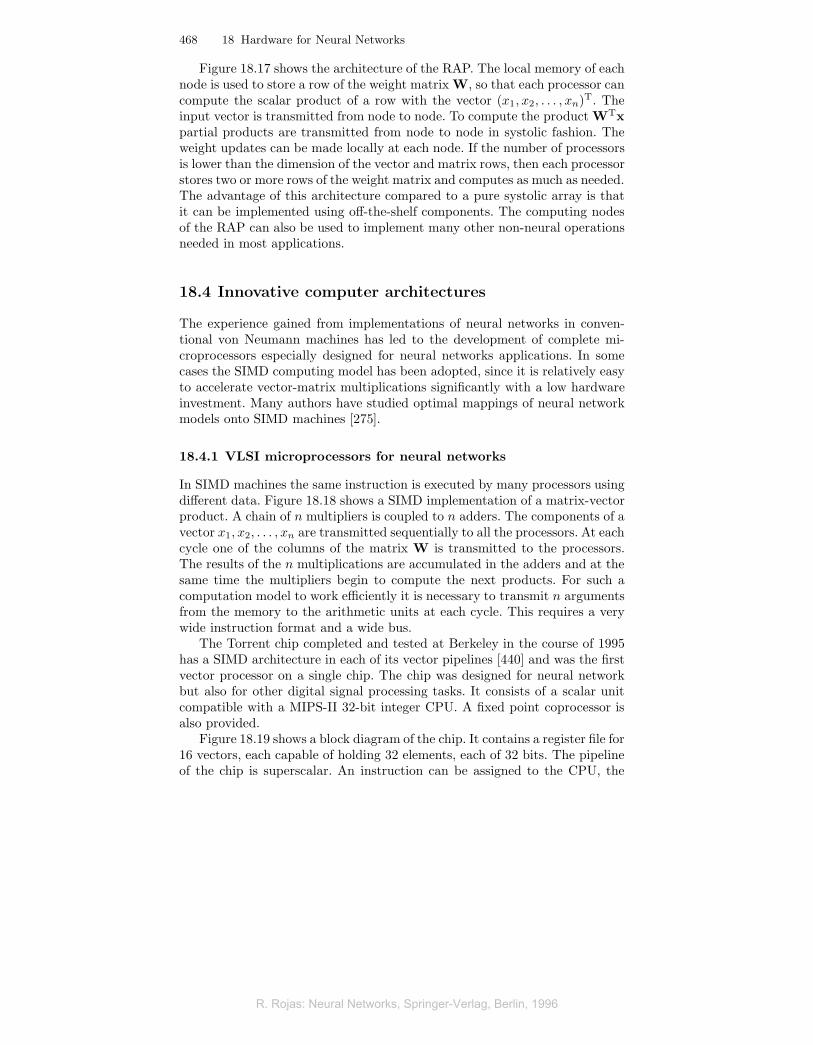
In SIMD machines the same instruction is executed by many processors usingdifferent data. Figure 18.18 shows a SIMD implementation of a matrix-vectorproduct. A chain of n multipliers is coupled to n adders. The components of avector x1, x2, . . . , xn are transmitted sequentially to all the processors. At eachcycle one of the columns of the matrix W is transmitted to the processors.The results of the n multiplications are accumulated in the adders and at thesame time the multipliers begin to compute the next products. For such acomputation model to work efficiently it is necessary to transmit n argumentsfrom the memory to the arithmetic units at each cycle. This requires a verywide instruction format and a wide bus.

The Torrent chip completed and tested at Berkeley in the course of 1995has a SIMD architecture in each of its vector pipelines [440] and was the firstvector processor on a single chip. The chip was designed for neural networkbut also for other digital signal processing tasks. It consists of a scalar unitcompatible with a MIPS-II 32-bit integer CPU. A fixed point coprocessor isalso provided.

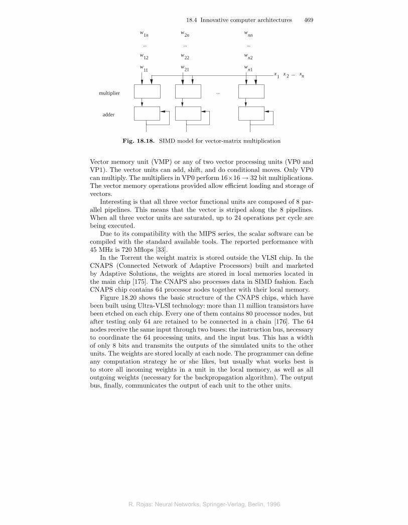
Figure 18.19 shows a block diagram of the chip. It contains a register file for16 vectors, each capable of holding 32 elements, each of 32 bits. The pipelineof the chip is superscalar. An instruction can be assigned to the CPU, the



18.4 Innovative computer architectures 469

multiplier

adder

w21

w22

w2n

...

wn1

wn2

wnn

...

w11

w12

w1n

...

...

x x x1 2 n...

Fig. 18.18. SIMD model for vector-matrix multiplication

Vector memory unit (VMP) or any of two vector processing units (VP0 andVP1). The vector units can add, shift, and do conditional moves. Only VP0can multiply. The multipliers in VP0 perform 16×16→ 32 bit multiplications.The vector memory operations provided allow efficient loading and storage ofvectors.

Interesting is that all three vector functional units are composed of 8 par-allel pipelines. This means that the vector is striped along the 8 pipelines.When all three vector units are saturated, up to 24 operations per cycle arebeing executed.

Due to its compatibility with the MIPS series, the scalar software can becompiled with the standard available tools. The reported performance with45 MHz is 720 Mflops [33].

In the Torrent the weight matrix is stored outside the VLSI chip. In theCNAPS (Connected Network of Adaptive Processors) built and marketedby Adaptive Solutions, the weights are stored in local memories located inthe main chip [175]. The CNAPS also processes data in SIMD fashion. EachCNAPS chip contains 64 processor nodes together with their local memory.

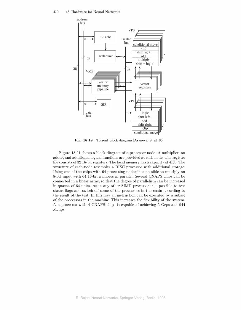
Figure 18.20 shows the basic structure of the CNAPS chips, which havebeen built using Ultra-VLSI technology: more than 11 million transistors havebeen etched on each chip. Every one of them contains 80 processor nodes, butafter testing only 64 are retained to be connected in a chain [176]. The 64nodes receive the same input through two buses: the instruction bus, necessaryto coordinate the 64 processing units, and the input bus. This has a widthof only 8 bits and transmits the outputs of the simulated units to the otherunits. The weights are stored locally at each node. The programmer can defineany computation strategy he or she likes, but usually what works best isto store all incoming weights in a unit in the local memory, as well as alloutgoing weights (necessary for the backpropagation algorithm). The outputbus, finally, communicates the output of each unit to the other units.




I-Cache

scalar unit

vectormemorypipeline

SIP

vectorregisters

scalarbus

addressbus

VMP

databus

conditional moveclip

shift rightadd

multiplyshift + logic

logicshift left

addshift right

clipconditional move

32

128

28

VP0

VP1

Fig. 18.19. Torrent block diagram [Asanovic et al. 95]

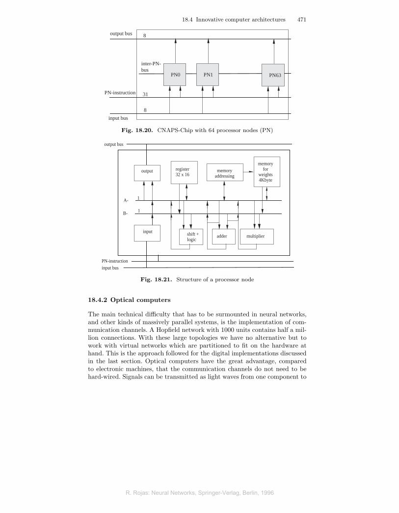
Figure 18.21 shows a block diagram of a processor node. A multiplier, anadder, and additional logical functions are provided at each node. The registerfile consists of 32 16-bit registers. The local memory has a capacity of 4Kb. Thestructure of each node resembles a RISC processor with additional storage.Using one of the chips with 64 processing nodes it is possible to multiply an8-bit input with 64 16-bit numbers in parallel. Several CNAPS chips can beconnected in a linear array, so that the degree of parallelism can be increasedin quanta of 64 units. As in any other SIMD processor it is possible to teststatus flags and switch-off some of the processors in the chain according tothe result of the test. In this way an instruction can be executed by a subsetof the processors in the machine. This increases the flexibility of the system.A coprocessor with 4 CNAPS chips is capable of achieving 5 Gcps and 944Mcups.




PN0 PN1 PN63

8

31

8

inter-PN-bus

output bus

input bus

PN-instruction

Fig. 18.20. CNAPS-Chip with 64 processor nodes (PN)

register32 x 16

memoryaddressing

memoryfor

weights4Kbyte

A-

B-

shift +logic

adder multiplier

1

1

output

output bus

input busPN-instruction

input

Fig. 18.21. Structure of a processor node

18.4.2 Optical computers

The main technical difficulty that has to be surmounted in neural networks,and other kinds of massively parallel systems, is the implementation of com-munication channels. A Hopfield network with 1000 units contains half a mil-lion connections. With these large topologies we have no alternative but towork with virtual networks which are partitioned to fit on the hardware athand. This is the approach followed for the digital implementations discussedin the last section. Optical computers have the great advantage, comparedto electronic machines, that the communication channels do not need to behard-wired. Signals can be transmitted as light waves from one component to




the other. Also, light rays can cross each other and this does not affect theinformation they are carrying. The energy needed to transmit signals is low,since there is no need to consider the capacity of the transmitting medium, asin the case of metal cables. Switching times of up to 30 GHz can be achievedwith optical elements [296].

SLM (50%) SLM (10%)

I 0,5 I 0,05 I

I

I

I + I1

2

1

2multiplication

addition

fan out

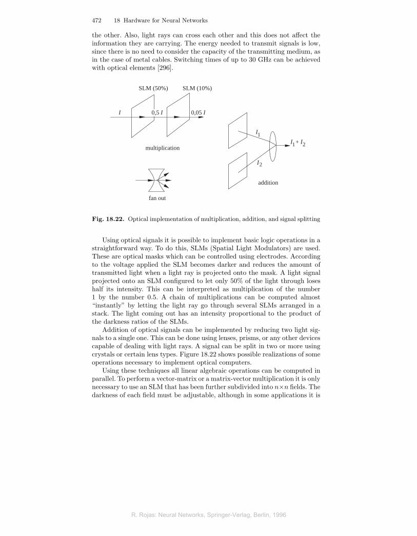
Fig. 18.22. Optical implementation of multiplication, addition, and signal splitting

Using optical signals it is possible to implement basic logic operations in astraightforward way. To do this, SLMs (Spatial Light Modulators) are used.These are optical masks which can be controlled using electrodes. Accordingto the voltage applied the SLM becomes darker and reduces the amount oftransmitted light when a light ray is projected onto the mask. A light signalprojected onto an SLM configured to let only 50% of the light through loseshalf its intensity. This can be interpreted as multiplication of the number1 by the number 0.5. A chain of multiplications can be computed almost“instantly” by letting the light ray go through several SLMs arranged in astack. The light coming out has an intensity proportional to the product ofthe darkness ratios of the SLMs.

Addition of optical signals can be implemented by reducing two light sig-nals to a single one. This can be done using lenses, prisms, or any other devicescapable of dealing with light rays. A signal can be split in two or more usingcrystals or certain lens types. Figure 18.22 shows possible realizations of someoperations necessary to implement optical computers.

Using these techniques all linear algebraic operations can be computed inparallel. To perform a vector-matrix or a matrix-vector multiplication it is onlynecessary to use an SLM that has been further subdivided into n×n fields. Thedarkness of each field must be adjustable, although in some applications it is




w

w

ww

w

w

w

w

w

w

w

w

w

w

w

w

11

21

31

41

12

22

32

42

43

33

23

13

14

24

34

44

x

x

x

x yy

y

y1

2

3

4

1

2

3

4

SLMinput vector

result

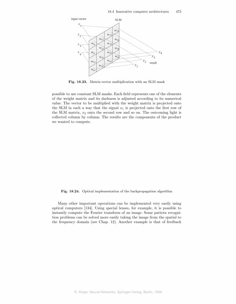
Fig. 18.23. Matrix-vector multiplication with an SLM mask

possible to use constant SLM masks. Each field represents one of the elementsof the weight matrix and its darkness is adjusted according to its numericalvalue. The vector to be multiplied with the weight matrix is projected ontothe SLM in such a way that the signal x1 is projected onto the first row ofthe SLM matrix, x2 onto the second row and so on. The outcoming light iscollected column by column. The results are the components of the productwe wanted to compute.

Fig. 18.24. Optical implementation of the backpropagation algorithm

Many other important operations can be implemented very easily usingoptical computers [134]. Using special lenses, for example, it is possible toinstantly compute the Fourier transform of an image. Some pattern recogni-tion problems can be solved more easily taking the image from the spatial tothe frequency domain (see Chap. 12). Another example is that of feedback




systems of the kind used for associative memories. Cellular automata can bealso implemented using optical technology. Figure 18.24 shows a diagram ofan experiment in which the backpropagation algorithm was implemented withoptical components [296].

The diagram makes the main problem of today’s optical computers evi-dent: they are still too bulky and are mainly laboratory prototypes still waitingto be miniaturized. This could happen if new VLSI techniques were developedand new materials discovered that could be used to combine optical with elec-tronic elements on the same chips. However, it must be kept in mind that just40 years ago the first transistor circuits were as bulky as today’s optical de-vices.

18.4.3 Pulse coded networks

All of the networks considered above work by transmitting signals encodedanalogically or digitally. Another approach is to implement a closer simulationof the biological model by transmitting signals as discrete pulses, as if theywere action potentials. Biological systems convey information from one neuronto another by varying the firing rate, that is, by something similar to frequencymodulation. A strong signal is represented by pulses produced with a highfrequency. A feeble signal is represented by pulses fired with a much lowerfrequency. It is not difficult to implement such pulse coding systems in analogor digital technology.

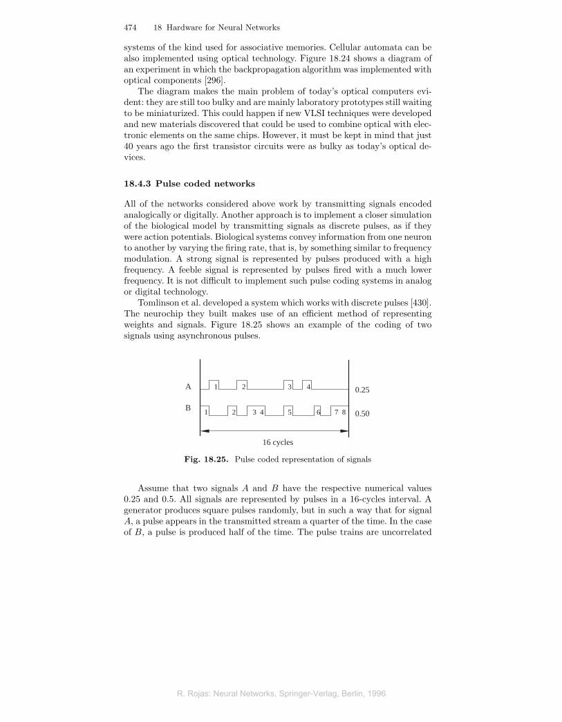
Tomlinson et al. developed a system which works with discrete pulses [430].The neurochip they built makes use of an efficient method of representingweights and signals. Figure 18.25 shows an example of the coding of twosignals using asynchronous pulses.

16 cycles

A

B

0.25

0.50

1 2 3 4

1 2 3 4 5 6 7 8

Fig. 18.25. Pulse coded representation of signals

Assume that two signals A and B have the respective numerical values0.25 and 0.5. All signals are represented by pulses in a 16-cycles interval. Agenerator produces square pulses randomly, but in such a way that for signalA, a pulse appears in the transmitted stream a quarter of the time. In the caseof B, a pulse is produced half of the time. The pulse trains are uncorrelated




to each other. This is necessary in order to implement the rest of the logicfunctions. A decoder can reconstruct the original numbers just by countingthe number of pulses in the 16-cycle interval.

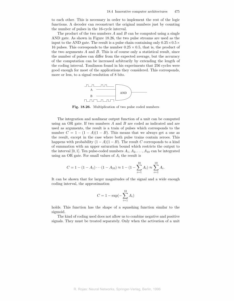
The product of the two numbers A and B can be computed using a singleAND gate. As shown in Figure 18.26, the two pulse streams are used as theinput to the AND gate. The result is a pulse chain containing only 0.25×0.5×16 pulses. This corresponds to the number 0.25× 0.5, that is, the product ofthe two arguments A and B. This is of course only a statistical result, sincethe number of pulses can differ from the expected average, but the accuracyof the computation can be increased arbitrarily by extending the length ofthe coding interval. Tomlinson found in his experiments that 256 cycles weregood enough for most of the applications they considered. This corresponds,more or less, to a signal resolution of 8 bits.

ANDA

B

Fig. 18.26. Multiplication of two pulse coded numbers

The integration and nonlinear output function of a unit can be computedusing an OR gate. If two numbers A and B are coded as indicated and areused as arguments, the result is a train of pulses which corresponds to thenumber C = 1 − (1 − A)(1 − B). This means that we always get a one asthe result, except in the case where both pulse trains contain zeroes. Thishappens with probability (1−A)(1−B). The result C corresponds to a kindof summation with an upper saturation bound which restricts the output tothe interval [0, 1]. Ten pulse-coded numbers A1, A2, . . . , A10 can be integratedusing an OR gate. For small values of Ai the result is

C = 1− (1− A1) · · · (1−A10) ≈ 1− (1−10∑

i=1

Ai) ≈10∑

i=1

Ai.

It can be shown that for larger magnitudes of the signal and a wide enoughcoding interval, the approximation

C = 1− exp(−10∑

i=1

Ai)

holds. This function has the shape of a squashing function similar to thesigmoid.

The kind of coding used does not allow us to combine negative and positivesignals. They must be treated separately. Only when the activation of a unit




has to be computed do we need to combine both types of signals. This requiresadditional hardware, a problem which also arises in other architectures, forexample in optical computers.

How to implement the classical learning algorithms or their variants us-ing pulse coding elements has been intensively studied . Other authors havebuilt analog systems which implement an even closer approximation to thebiological model, as done for example in [49].

18.5 Historical and bibliographical remarks

The first attempts to build special hardware for artificial neural networksgo back to the 1950s in the USA. Marvin Minsky built a system in 1951that simulated adaptive weights using potentiometers [309]. The perceptronmachines built by Rosenblatt are better known. He built them from 1957 to1958 using Minsky’s approach of representing weights by resistances in anelectric network.

Rosenblatt’s machines could solve simple pattern recognition tasks. Theywere also the first commercial neurocomputers, as we call such special hard-ware today. Bernard Widrow and Marcian Hoff developed the first series ofadaptive systems specialized for signal processing in 1960 [450]. They useda special kind of vacuum tube which they called a memistor. The Europeanpioneers were represented by Karl Steinbuch, who built associative memoriesusing resistance networks [415].

In the 1970s there were no especially important hardware developmentsfor neural networks, but some attempts were made in Japan to actually buildFukushima’s cognitron and neocognitron [144, 145].

Much effort was invested in the 1980s to adapt conventional multiprocessorsystems to the necessities of neural networks. Hecht-Nielsen built the series ofMark machines, first using conventional microprocessors and later by devel-oping special chips. Some other researchers have done a lot of work simulatingneural networks in vector computers or massively parallel systems.

The two main fields of hardware development were clearly defined in themiddle of the 1980s. In the analog world the designs of Carver Mead and hisgroup set the stage for further developments. In the digital world many alter-natives were blooming at this time. Zurada gives a more extensive descriptionof the different hardware implementations of neural networks [469].

Systolic arrays were developed by H. T. Kung at Carnegie Mellon in the1970s [263]. The first systolic architecture for neural networks was the Warpmachine built at Princeton. The RAP and Synapse machines, which are notpurely systolic designs, nevertheless took their inspiration from the systolicmodel.

But we are still awaiting the greatest breakthrough of all: when will opticalcomputers become a reality? This is the classical case of the application, the



18.5 Historical and bibliographical remarks 477

neural networks, waiting for the machine that can transform all their promisesinto reality.

Exercises

1. Train a neural network using floating-point numbers with a limited preci-sion for the mantissa, for example 12 bits. This can be implemented easilyby truncating the results of arithmetic operations. Does backpropagationconverge? What about other fast variations of backpropagation?

2. Show how to multiply two n×n matrices using a two-dimensional systolicarray. How many cycles are needed? How many multipliers?

3. Write the pseudocode for the backpropagation algorithm for the CNAPS.Assume that each processor node is used to compute the output of a singleunit. The weights are stored in the local memory of the PNs.

4. Propose an optical system of the type shown in Figure 18.23, capable ofmultiplying a vector with a matrix W, represented by an SLM, and alsowith its transpose.




.



Documents

18 Hardware for Neural Networks - UserPages < Tec < …page.mi.fu-berlin.de/rojas/neural/chapter/K18.pdfR. Rojas: Neural Networks, Springer-Verlag, Berlin, 1996 452 18 Hardware for