Chapter 13: Applying scale transition theory to metacommunities in

Chapter 13: Applying scale transition theory to metacommunities in the field Affiliations: Brett A. Melbourne Center for Population Biology, University of California, Davis Anna L. W. Sears Center for Population Biology, University of California, Davis Megan J. Donahue Section of Evolution and Ecology, University of California, Davis Peter Chesson Section of Evolution and Ecology, University of California, Davis Mailing Address:

Brett Melbourne Environmental Science and Policy Wickson Hall University of California, Davis, CA 95616

Phone (530) 752-6837, (530) 754-9734 Fax (530) 752-3350 [email protected] Short title: Applying scale transition theory Revised accepted: 25 October 2003 Proofed: 11 March 2005 Citation: Melbourne BA, Sears AL, Donahue MJ, Chesson P (2005). Applying scale transition theory to metacommunities in the field. In M. Holyoak, M. A. Leibold and R. D. Holt eds. Metacommunities: Spatial Dynamics and Ecological Communities. Chicago, University of Chicago Press, pp 307-330.

Preprint, same as printed version 11 March 2005.

13.1

Chapter 13: Applying scale transition theory to metacommunities in the field

Brett A. Melbourne, Anna L. W. Sears, Megan J. Donahue and Peter Chesson

Introduction A metacommunity consists of local communities linked by dispersal. This concept distinguishes between community processes that operate at local spatial scales and dispersal processes that link local communities together. The dynamics of the metacommunity as a whole result from an interplay between these local and regional processes, affecting dynamical outcomes such as stability, competitive exclusion, and persistence (Bolker and Pacala 1997; Chesson 2000; De Jong 1979; Hassell et al. 1991; Ives 1988; Pacala and Levin 1997). The major issue in metacommunity studies is understanding how regional dynamics arise from local dynamics, in other words, scaling up from the dynamics of local communities to the larger spatial scale of the metacommunity. In the chapter on scale transition theory (Chesson et al., chapter 12), we saw that the rules that determine community dynamics change as our view shifts from the small spatial scale of the local community to the larger spatial scale of the metacommunity. The key determinants of these changes were shown to be spatial variation between local communities and nonlinearity in local processes, neither being important without the other. Indeed, it is the interaction between spatial variation and nonlinearity that underpins the changes. Spatial heterogeneity is ubiquitous to ecological systems: we know from field experience that the density of each species, their resources, competitors, and predators vary over space. By nonlinearities, we mean that the relationship between population growth rate and the density of conspecifics, resources, competitors, or predators is nonlinear. Nonlinearities are also ubiquitous to ecological systems. For example, local per capita growth rates that depend on environmental conditions, or the simple act of one species feeding on another, involve nonlinearities. Any source of density dependence, such as intra- or inter-specific competition, also involves a nonlinearity. The critical insight of scale transition theory is that spatial variation between local communities, and nonlinearities within local communities, interact to determine the dynamics of the metacommunity. Through this insight, scale transition theory systemizes the study of metacommunities by identifying key quantities, which represent spatial mechanisms, that contribute to change with spatial scale. The spatial storage effect and fitness-density covariance are two examples of such mechanisms (Chesson 2000; Chesson et al., chapter 12). The presence and magnitude of these mechanisms also provides evidence that metacommunity processes are important to the dynamics of the metacommunity. If these mechanisms are absent we would expect little difference in dynamics between local-scale communities and metacommunities, that is, linking local communities together by dispersal would have little consequence. In this chapter we show how to apply scale transition ideas, as presented in the theory chapter 12 using examples from three quite different field systems. There are three steps to implement this research program: 1) derive a model to translate the effects of local dynamics to the metacommunity scale and to identify key interactions between nonlinearity and

Melbourne BA, Sears AL, Donahue MJ, Chesson P. (2005). Applying scale transition theory to metacommunities in the field. In M. Holyoak, M. A. Leibold and R. D. Holt eds. Metacommunities: Spatial Dynamics and Ecological Communities. Chicago, University of Chicago Press, pp 307-330.

13.2

spatial variation; 2) measure nonlinearities at local scales; and 3) measure spatial variances and covariances. We show how to work through each of these steps and how to combine the models and data to calculate effects on dynamics at the metacommunity scale. Our field examples demonstrate a range of dynamical outcomes that result from a metacommunity structure. The first two field examples focus on a single species or functional group within a metacommunity but include interactions with other trophic levels. These first two examples are perhaps best considered metapopulation studies but they serve as a bridge to demonstrate how scale transition tools are applied to metacommunities. The final example is for competition between two species of annual plants. In all three examples, considering the spatial context of the metacommunity allows a deeper understanding of the mechanics of the system.

Example 1: benthic algae and grazers on stream cobbles The first field example is for the dynamics of benthic algae growing on stream cobbles and grazed by insect larvae. Recently, stream systems, and the algae-grazer system in particular, have inspired much interest in the issue of heterogeneity and scaling because of high spatial variation in the density of organisms and physical conditions (Cooper et al. 1997, 1998; Downes et al. 1993; Nisbet et al. 1997). Melbourne and Chesson (submitted) described a study of the scale transition for algae (more accurately periphyton dominated by algae) and grazers in a stream system in southeastern Australia. In these streams, algal assemblages were dominated by diatoms and green algae and were consumed mainly by the aquatic larval stages of caddisfly, mayfly and waterpenny species. Interactions between algae and grazers occur in local patches, on centimeter scales, yet we wish to scale up to a metacommunity scale that encompasses the entire study area, some 42 km of stream. What role does spatial structure play in this system? How big might the effects of spatial structure and spatial variation be on algal-grazer dynamics at the larger scale of the stream?

Model to scale up algae and grazers It is worth going into some detail to show how models were derived to scale up from local processes at the scale of centimeter-sized patches to the regional scale of the stream. We begin by formulating a model for the dynamics of algae and grazers at the local scale. We treat algae and grazers as functional groups, not differentiating the separate dynamics of each species but instead examining the overall dynamics of algae and grazers. At the local scale, algal dynamics are determined by three processes: algal growth, consumption by grazers, and dispersal of algae into and out of a location. Here we use the patch model formulation of the scale transition (Chesson et al., chapter 12, equation 12.10). A simple model for algal dynamics at location x (a small patch, say 2 cm in diameter) is thus

( ) ( ) ,,A,A xxxxx

x IGAfAgdt

dA ε−+−= (13.1)

where A is the density of algae (biomass per unit area), t is time, and G is the density of grazers (biomass per unit area). The model is a standard balance equation plus dispersal terms, where g(A) is a function that describes algal growth rate (biomass per unit area per unit time) as a function of algal density, and f(A)G describes the rate of algal consumption by grazers, where


13.3

f(A) is the functional response of a grazer. In writing consumption as f(A)G, we are assuming that grazer consumption is linear in G, which means that grazers do not interact with each other directly through interference but only indirectly by consuming algae, a standard assumption for this system (Nisbet et al. 1997). Algal dispersal to and from location x is modeled by the generic functions IA,x and εA,x, to which we can assign any set of dispersal rules (provided that dispersal mortality is factored into the growth rate terms [Chesson et al., chapter 12]). For example, algal immigration rate, IA, at location x might depend on the output from nearby patches or the vagaries of stream currents, and algal emigration rate, εA, at location x might depend on algal density at that location. Equation 13.1 is in continuous time, which matches the nature of algal dynamics. A simple model for grazer dynamics at location x is

( )( ) ,,G,G xxxxx IGmAcf

dtdG ε−+−= (13.2)

where c is the conversion efficiency of grazers, m is grazer mortality, and grazer movement is modeled by the generic functions IG,x and εG,x. Thus, a model for the local dynamics of algae and grazers consists of the coupled equations 13.1 and 13.2. To match the time scale that can be achieved in field experiments (i.e. two to three weeks), we reformulate the model for grazer dynamics to a short time scale, over which the net gain in grazer density due to the consumption of algae is trivial (Nisbet et al. 1997). Thus, we set [cƒ(Bx)-m]Gx = 0, and the local dynamics of grazers is determined only by movement into and out of the location. For example, such movement might be a result of foraging decisions made by individual grazers (recall that a location is a 2 cm diameter patch), or a response to environmental conditions or predators at the location, or upstream or downstream movement in response to stream flow. To fully specify the model, we need to put forward specific functions for g(A) and f(A) but for now we leave the model in its general form and proceed to the scaling up step. As we will see, we do not need to specify the algal dispersal and grazer movement functions. We wish to scale up to find the dynamics for the entire stream. At this regional scale, we consider the system to be effectively closed, meaning that the rate of dispersal across the boundaries is so small that it can have no effect on internal dynamics. Over short time scales, this is an especially realistic assumption for streams. The entire stream encompasses the headwaters, so there is no immigration from upstream and there is no immigration from the surrounding terrestrial environment. The only dispersal that occurs across the stream boundaries is at the downstream end, where the amount of dispersal across the stream boundary is tiny compared to that within the system upstream. We consider only short time scales here but over longer time scales we might need to deal with flood events, when there can be a large export of algae and grazers from the system at the downstream end. To scale up from local, centimeter sized patches, to the regional scale of a stream, where patches (indexed by x) are now linked by dispersal of algae and movement of grazers, we average the local dynamics over all patches. This regional average is a foundation of the scale transition: the average of the local densities is in fact the regional density (Chesson et al., chapter 12). Thus, averaging over both sides of equations 13.1 and 13.2, the regional dynamics are


13.4

( ) ( ) ( ) ( )

( ) ( )

,0GGGG

AAAA

=−=−=

−=

−+−=−+−=

εε

εε

IIdtGd

GAfAg

IGAfAgIGAfAgdtAd

(13.3)

where the overbars indicate an average over space, and the subscript x disappears because that is what we are averaging over. The overbar extends all the way across the right hand side, indicating that the rate of change in algal density at the regional scale is an average of the local functions for growth, consumption, and dispersal. As averages are additive, the regional average simplifies to the separate averages for growth, consumption, and dispersal (equation 13.3). Since the system is effectively closed at the regional scale, individuals leaving one location within the region enter another location, so that the total number of individuals leaving locations is equal to the total number of individuals entering locations (i.e., 0=− εI ). Thus the dispersal functions disappear and dispersal within the system becomes an implicit part of the model, rather than appearing explicitly at the regional scale. Equation 13.3 is our fundamental equation for the regional dynamics and we can now work through it to find a useful expression for the scale transition by using the properties of nonlinear averages given in chapter 12, box 2. The average of the product ( )GAf in equation 13.3 splits into the product of the averages and the covariance in space between them (chapter 12, equation 12.B2.6), so

( ) ( ) ( )( )GAfGAfAgdtAd ,Cov−−= . (13.4)

At this stage, the equation still gives the exact dynamics for the region. Thus, in equation 13.4 it can be seen that the dynamics for the region involves the covariance over space between grazer functional response and grazer density. The grazer functional response will vary in space according to variation in algal density between locations. By approximating g(A) and f(A) as second order Taylor polynomials (chapter 12, equation 12.B2.5), we get

( ) ( ) ( ) ( ) ( ) ( ) ( )( ),,CovVar21Var

21 GAfGAAfAfAAgAg

dtAd

−⎟⎠⎞

⎜⎝⎛ ′′+−⎟

⎠⎞

⎜⎝⎛ ′′+= (13.5)

where Var(A) is the variance of A over space and ( )Ag ′′ and ( )Af ′′ are the second derivatives of ( )Ag and ( )Af . Finally, rearranging and taking a linear approximation for f(A) in the

covariance term (chapter 12, equation 12.B2.8) we get

( ) ( ) ( ) ( ) ( ) ( ) ( ) ( ),,CovVar21Var

21

cba

model fieldmean44 344 21

44 344 2144 344 2144 344 21 GAAfAGAfAAgGAfAg

dtAd ′−′′−′′+−=

−

(13.6)

where ( )Af ′ is the first derivative of ( )Af . The structure of this model for the regional dynamics is very informative and empirically useful. The first two terms are the mean field model, which is simply the equation for local dynamics (equation 13.1 without dispersal) with


13.5

the mean density across patches substituted for local density. We can think of the mean-field model as representing local dynamics. The regional dynamics are thus given by the mean field model plus three scale transition terms (a-c) that correct the mean field model to account for spatial structure. Most importantly, equation 13.6 tells us what we need to measure in field studies: the nonlinearities in algal growth and grazer consumption expressed by g''(A) and f''(A), the spatial variance of algal density, Var(A), and the spatial covariance of algal and grazer density, Cov(A,G). Here nonlinear means that the rate of algal growth or consumption varies as a nonlinear function of algal density (discussed below). To analyze the consequences of the metapopulation structure, we consider the magnitude and sign of the terms (a-c) relative to the mean-field model and to each other. Terms (a) and (b) are a consequence of spatial variation in algal density between patches and clearly demonstrate how changing scale involves an interaction between nonlinearity and spatial variation, since they involve the product of 1) the second derivative g''(A) or f''(A), which measure nonlinearities in the local processes of algal growth or grazer functional response respectively, and 2) the variance in algal density between locations, Var(A). For algal growth, g(A), local nonlinearities might result from competition for resources within the algal film. For example, as algal density increases, shading by overlying algal cells reduces the photosynthetic rate of cells in layers below, resulting in density dependent growth. For the functional response of grazers, f(A), local nonlinearities might result from a handling time requirement or an attack rate that varies with algal density, for example, as in a classic Type II or Type III functional response. Depending on the sign of the second derivatives ( )Ag ′′ and ( )Af ′′ , which are determined by whether each function is concave down (negative second derivative) or concave up (positive second derivative), the nonlinearities may work either in opposing directions, thus moderating the effect of variation, or in the same direction, thus compounding the effect of variation on regional dynamics. The third term (c) also results from an interaction between nonlinearity and spatial variation but the interaction is now due to the two-dimensional nonlinearity of algae and grazer density. This nonlinearity is simply because grazers eat algae. Spatial variation in G alone does not appear in the regional model and the effect of spatial variation in G enters only through spatial covariation with A. This is because we assume that grazer consumption is linear in G (equation 13.1). The influence of spatial variation in grazer density on the scale transition depends on the covariance between algae and grazer density (term c), in other words, on how algae and grazers are distributed in space in relation to one another. While dispersal of algae and movement of grazers within the system are explicit in the construction of the model, they do not appear in equation 13.6. Instead, the effects of dispersal and movement on the spatial pattern are represented by the variance and covariance terms. For example, the movement of grazers affects these terms because grazers move around in the stream, eating algae, thus creating (or destroying) variation in algal density. Similarly, movement and consumption could set up covariance between algae and grazer density. Thus, while dispersal of algae and movement of grazers does not appear in the regional model (indeed an equation for the dynamics of grazers does not appear at all), the model incorporates the effects of algal dispersal and grazer movement within the system.


13.6

We know that this system consists of local patches in the stream that are linked by dispersal of algae and movement of grazers. If this metapopulation structure is important in explaining dynamics at the larger scale of the stream, then we should be able to detect and quantify the interactions (a-c) in the field. That requires measuring the nonlinearities associated with algal growth and grazer consumption as well as the variances and covariance in equation 13.6.

Measuring nonlinearities in algae and grazers In general, local nonlinearities can be estimated by varying levels of the nonlinear factors (usually population density) in an experiment and fitting models to the experimental data to describe the shape of the nonlinearities. This same general approach is applied to all three field examples in this chapter, although the methodological details are peculiar to the processes and experimental constraints of the different systems. To measure nonlinearities in the algae-grazer system, we need to put forward specific functional forms for algal growth and grazer foraging. Recall that nonlinear means that the rate of algal growth or consumption varies as a nonlinear function of algal density. It is useful in this step to put forward alternative models as hypotheses for the functional form and to test between models by confronting them with experimental data, as described in Melbourne and Chesson (submitted ms). To measure nonlinearities in algal growth, the experiment involved excluding grazers from rocks in the stream and examining the growth of algae in centimeter-sized patches in the absence of grazers, over a range of initial density for the algae. The functional response of grazers was determined similarly by examining consumption over a range of algal densities in the stream. The best-fitting models were the logistic model for algal growth and the Type III functional response for grazers. These models, parameterized from the local scale data, characterize the nonlinearities in the process of algal growth g(A) and grazer consumption f(A) at local scales.

Measuring spatial variances and covariances Measuring spatial variation at the scale of local nonlinearities is critical to estimating the scale transition. We need to first identify the scale of the local nonlinearity, which is defined as the range of space over which the influence of the nonlinear process is homogeneous (the ecological neighborhood sensu Addicott et al. 1987). For a density dependent process, like algal growth, this scale is the scale of density dependence (Chesson 1996, 1998a). These scales can be tricky to determine precisely but their order of magnitude is often obvious. In the algae-grazer system, the different scales are the scale of competition between algal cells (on the order of micrometers to millimeters) and the scale of the grazer consumption process (on the order of centimeters to meters). We set the scale of algal growth to the smallest scale we could measure, which corresponded to our algal sampling device (2.4 cm diameter). For the scale of grazer consumption, we also assume the smallest scale we could measure (2.4 cm diameter), meaning that grazers can perceive and respond to variation in algal density between centimeter-sized patches. To measure the spatial variance of algal density and the spatial covariance for algal and grazer density, samples of algae and grazer density were taken in a hierarchical sampling design and the total variance and covariance at the scale of the local nonlinearity was estimated by analysis of the variance components (Melbourne and Chesson submitted; Searle et al. 1992; Underwood and Chapman 1996).


13.7

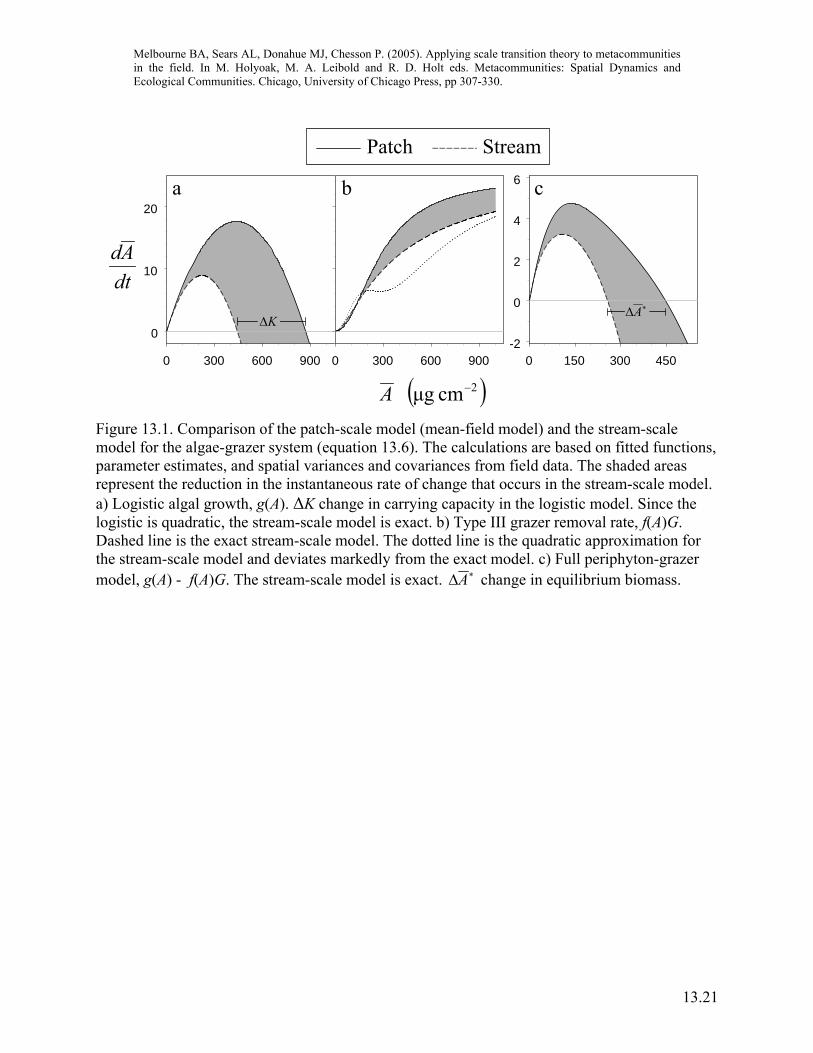
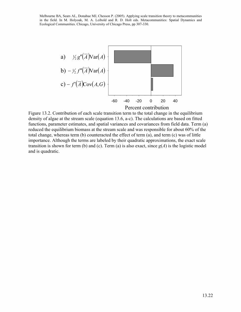
Combining the model with field data to scale up Having identified models and estimated parameters for the nonlinear functions for algal growth and grazer foraging, and estimated the spatial variances and covariance in equation 13.6, we can now scale up the dynamics from the local scale of a centimeter-sized patch, where interactions between individuals take place, to the scale of the stream, which is made up of patches linked by dispersal of algae and movement of grazers. A note of caution is required here. The approximations in equation 13.6 give the trend as the variance increases from zero, but if the equations are not quadratic, the approximation may become inaccurate when the spatial variance is large. The logistic model for algal growth is exactly quadratic but the Type III functional response for grazers departs markedly from a quadratic and the approximation breaks down because we observe high variance (figure 13.1). For the Type III response, we calculated the exact scale transition for terms (b) and (c) in equation 13.6, as described in Melbourne and Chesson (submitted). The effect of scaling up is to reduce the instantaneous rate of growth at the stream scale compared to local patches (figure 13.1). That is, for a given algal density at the stream scale, growth is reduced compared to growth for the same algal density at the patch scale. The area shaded in gray in figure 13.1 represents the scale transition: the difference in output from the patch-scale population dynamics (given by the mean-field curve) and the spatial model for the stream that takes into account the metapopulation structure. The metapopulation structure doesn’t qualitatively alter aspects of the short term dynamics, such as the stability because the general form of the spatial model is still a hump-shaped curve (figure 13.1). However, an important basic property that is quantitatively altered is the equilibrium density of algae, ∗A , the balance of growth and consumption. This short term equilibrium density is reduced at the stream scale by about 41%, a substantial reduction (figure 13.1). Thus, spatial variation and nonlinearity interact to reduce algal density at the metapopulation scale. Recall that the important components that arise because of the metapopulation structure are the terms (a-c) in equation 13.6 that represent interactions between nonlinearity and spatial variance. When we look at the three components of the scale transition, the main effect is seen to be from the interaction of nonlinearity in algal growth with spatial variation in algal density (figure 13.2), because both the nonlinearity and the variance were high. This effect is offset somewhat by the interaction between the nonlinear functional response with spatial variation in algal density (figure 13.2). Nonlinearity in the functional response was less than for algal growth, so the offset is smaller than the algal growth term. The spatial covariance of algae and grazers was negative but the covariance term was too small to influence the outcome (figure 13.2). Thus, by examining these relative contributions we can determine the most important spatial mechanisms that alter dynamics at the regional scale. This example demonstrates the basic concepts and properties of the scale transition in translating the effects of local scale processes to the scale of the metapopulation, where locations are linked by dispersal. Scale transition theory identified the important component mechanisms that change dynamics at the metapopulation scale. These components were then possible to measure


13.8

relatively easily by applying standard field experiments and sampling designs. We confirmed that metapopulation processes were important to the dynamics of the system because we detected large scale transition components. Had we not detected such large components, we would not expect the metapopulation structure to have any important effects on dynamics at the larger scale of the stream, the stream would act much like a patch. The next field example involves a greater variety of local processes than the simple example above, demonstrating that more complicated cases are approached in the same way.

Example 2: dynamics of an intertidal crab The second field example is for the dynamics of an intertidal crab that, like many other marine organisms, has a planktonic larval stage. Current research in marine ecology recognizes that marine systems are metacommunities, in which local populations and communities are interconnected through larval dispersal (Armsworth 2002; Chesson 1998b; Jones et al. 1999; Swearer et al. 1999, 2002; Thorrold et al. 2002). This metacommunity view contrasts with a “supply-side” perspective of marine systems, in which larval supply is treated as an external force that sets the stage for subsequent local dynamics but does not feedback to the larval pool (Gaines and Roughgarden 1985; Grosberg and Levitan 1992). When marine systems are viewed as a metacommunity, larval supply is not an external force on local communities but interacts with local processes to influence local and metacommunity dynamics (Armsworth 2002; Chesson 1998b). In our example system, the porcelain crab, Petrolisthes cinctipes, lives under rocks in intertidal cobblefields in the northeast Pacific. It releases larvae that feed and develop in the plankton for 1-2 months. Upon returning to adult habitat, the larvae settle and, if they survive high post-settlement mortality, recruit to the adult population (Donahue 2003; Jensen 1989, 1991). Adults are filter-feeders and live in aggregations under rocks. Rocks are relatively discrete habitat patches because P. cinctipes move little unless their rock is disturbed. There are two natural scales of variation to consider: rocks (rock area≈0.1m2) within sites, and sites (site length≈1 km) within the metacommunity that encompasses the coastline. Competitive interactions between crabs occur at the rock scale. Predators forage across rocks within sites. Sites are connected by larval dispersal. We model larval distribution in the following way: larvae generated at all sites enter a larval pool and the proportion of this larval pool distributed to a particular site is a site-scale characteristic. We wish to scale up from rock- and site-scale interactions to the metapopulation that encompasses the coast.

Model to scale up crab dynamics We begin by formulating a model for the dynamics of P. cinctipes at the cobble scale, where interactions between individuals take place. The important population processes can be divided into recruitment and adult growth. Juveniles settle gregariously in response to adult density (Donahue submitted ms; Jensen 1989). To recruit, settlers must survive predation from resident predators (several species of fish and crabs) (Donahue 2003; Jensen 1991) and competition from resident adults (Donahue 2004). For adult crabs, growth rate and fecundity depend on


13.9

conspecific density (Donahue 2004). These processes lead to a general model for the dynamics of crab biomass, Nx, under cobble x from the release of larvae in one season, t, to the release of larvae in the next t+1:

( ) ( ) ( )( ) ( ) ( ) ( )( )tLtPtNhtNgtNtN xxxxxx ,,1 ++=+ . (13.7)

In this model, g(Nx(t)) is a function that describes the density dependent growth and mortality of adult crabs and h is a function that describes recruitment. Recruitment is determined by the biomass of adults under the rock, Nx(t), the biomass of predators, Px(t), and larval supply, Lx(t), the total biomass of larvae delivered to the site. The larvae Lx(t) are the dispersed offspring of the adults present in the system at time t: Adults from cobble x produce bNx(t) new larvae, which disperse and become the inputs Lx(t) to equation 13.7. The equation implicitly assumes that dispersal is instantaneous. In reality it is spread out over time during the interval t to t + 1, with equation 13.7 being most accurate if dispersal is concentrated early in the time interval. Dispersal of larvae between sites could follow any mode of dispersal. For example, larvae could enter a global pool and disperse to sites according to ( )tNbUtL xx =)( , where Ux is the proportion of the regional larval pool delivered to the site (see also equation Chesson et al., chapter 12, equation 12.13). As the transition from adults to larvae is linear, we focus on the stage transition from larvae to adults in equation 13.7. Adult growth and competition take place at the rock-scale, while recruitment has both site-scale (larval supply, predator abundance) and rock-scale (competition, gregarious settlement) factors. To fully specify the model, we need specific functions for g and h but as in the previous example, we leave the model in its general form and proceed to the scaling up step. To understand regional dynamics in this system, we take spatial averages of both sides of this equation:

( ) ( ) ( )( ) ( ) ( ) ( )( )tLtPtNhtNgtNtN ,,1 ++=+ . (13.8)

The spatial average of the right-hand side can be approximated by a Taylor expansion. Since our general model is a function of three variables, we perform our Taylor expansion around mean adult density, mean predator density, and mean larval supply, each of which generate variance and covariance terms. Note that we are not tracking the dynamics of predators, but predator density influences attack rates.


13.10

( ) ( ) ( )( ) ( ) ( ) ( )( )

( ) ( ) ( )

( ) ( )

( ) ( ).,Cov,Cov

,CovVar21

Var21Var

21Var

21

,,1

g

,

2

f

,

2

e

,

2

d

2

2

c

2

2

b

2

2

a

2

2

model field-mean

444 3444 21444 3444 21

444 3444 2144 344 21

44 344 2144 344 2144 344 21

444444 3444444 21

LPLP

hLNLN

h

PNPN

hLLh

PPhN

NhN

Ng

tLtPtNhtNgtNtN

LPLN

PNL

PNN

∂∂∂

+∂∂

∂+

∂∂∂

+∂∂

+

∂∂

+∂∂

+∂∂

+

++≈+

(13.9)

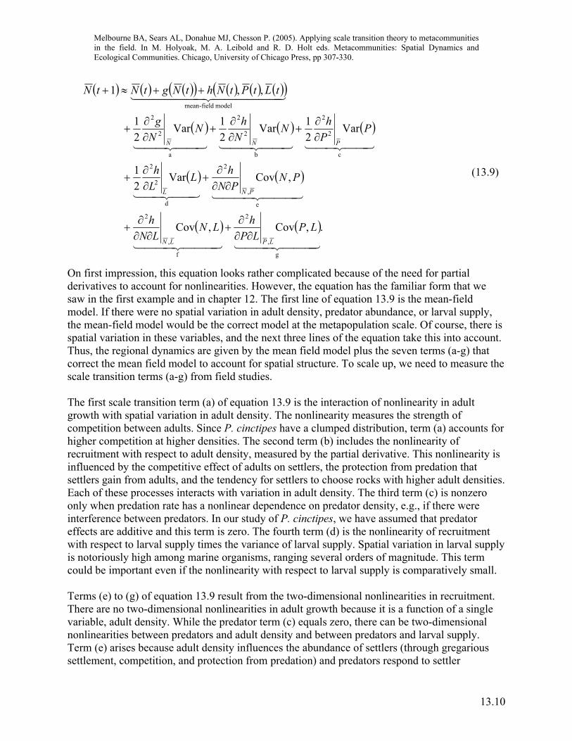
On first impression, this equation looks rather complicated because of the need for partial derivatives to account for nonlinearities. However, the equation has the familiar form that we saw in the first example and in chapter 12. The first line of equation 13.9 is the mean-field model. If there were no spatial variation in adult density, predator abundance, or larval supply, the mean-field model would be the correct model at the metapopulation scale. Of course, there is spatial variation in these variables, and the next three lines of the equation take this into account. Thus, the regional dynamics are given by the mean field model plus the seven terms (a-g) that correct the mean field model to account for spatial structure. To scale up, we need to measure the scale transition terms (a-g) from field studies. The first scale transition term (a) of equation 13.9 is the interaction of nonlinearity in adult growth with spatial variation in adult density. The nonlinearity measures the strength of competition between adults. Since P. cinctipes have a clumped distribution, term (a) accounts for higher competition at higher densities. The second term (b) includes the nonlinearity of recruitment with respect to adult density, measured by the partial derivative. This nonlinearity is influenced by the competitive effect of adults on settlers, the protection from predation that settlers gain from adults, and the tendency for settlers to choose rocks with higher adult densities. Each of these processes interacts with variation in adult density. The third term (c) is nonzero only when predation rate has a nonlinear dependence on predator density, e.g., if there were interference between predators. In our study of P. cinctipes, we have assumed that predator effects are additive and this term is zero. The fourth term (d) is the nonlinearity of recruitment with respect to larval supply times the variance of larval supply. Spatial variation in larval supply is notoriously high among marine organisms, ranging several orders of magnitude. This term could be important even if the nonlinearity with respect to larval supply is comparatively small. Terms (e) to (g) of equation 13.9 result from the two-dimensional nonlinearities in recruitment. There are no two-dimensional nonlinearities in adult growth because it is a function of a single variable, adult density. While the predator term (c) equals zero, there can be two-dimensional nonlinearities between predators and adult density and between predators and larval supply. Term (e) arises because adult density influences the abundance of settlers (through gregarious settlement, competition, and protection from predation) and predators respond to settler


13.11

abundance. Therefore, there is a two-dimensional nonlinearity between predators and adult density. Term (f) arises because of gregarious settlement, in which larval supply interacts with adult density. Finally, term (g) arises because predators respond to prey density, and larval supply influences prey density. Each of the two-dimensional nonlinearities is multiplied by its respective covariance term.

Measuring local nonlinearities Our next goal was to empirically evaluate each component of this model. Since we wanted to estimate the functions for adult growth, g(N(t)), and larval recruitment, h(N(t),P(t),L(t)), we needed to perform growth and recruitment experiments over a range of densities. Starting with the growth component, we tested for intraspecific competition by tracking individual growth rates over a range of crab densities in field and laboratory experiments. We found that growth rate declined with increasing density and that smaller individuals were more strongly impacted by competition than large individuals (Donahue 2004). Since our general model has only two size classes, we incorporated size-specific competition by fitting a different competition coefficient for adults on settlers than adults on other adults. Competition is a nonlinearity with respect to adult density in both the growth and recruitment components of equation 13.9. Previous studies indicated that P. cinctipes settle preferentially with conspecifics (Jensen 1989). To quantify gregarious settlement, we manipulated adult density in field enclosures and counted the number of settlers to each enclosure (Donahue 2003). We performed this experiment during two settlement pulses to see how larval supply influenced the settlement pattern. We found that the per capita rate of settlement increased then saturated with adult density. This generates nonlinearity with respect to adult density. Settlers remain under adults and are protected from predation by this behavior (Jensen 1991). One model for this interaction is a decline in attack rate as the ratio of adults to settlers increases (Donahue 2003). We assume there is no interference between predators. This generates nonlinearity with respect to adult density and larval supply, but only two-dimensional nonlinearities with respect to predators.

Measuring spatial variances and covariances With models of density dependence established and parameterized, we measured variation in adult density, predator density, and supply at the appropriate scales. Variation in adult density is at the rock scale, while variation in predator density and larval supply is at the site scale. At fourteen cobblefield sites, we sampled forty rocks for adult crabs and predators. Since predators were less abundant, we sampled an additional eighty rocks for predators. From this, we could estimate the rock-scale and site-scale variance in adult density, Var(N), site-scale variance in predator abundance, Var(P), and site-scale covariance between adults and predators, Cov(N,P). At eight sites, we sampled larval supply using nearshore collectors and estimated the site-scale variance in larval supply, Var(L), and the site-scale covariances between density and supply, Cov(N,L), and between predator abundance and supply, Cov(P,L). Within a site, we consider supply to rocks and predator density at each rock within a single site to be uniform and,


13.12

therefore, there is no contribution of variance (or covariance) from the rock-scale that contributes to site-scale variance.

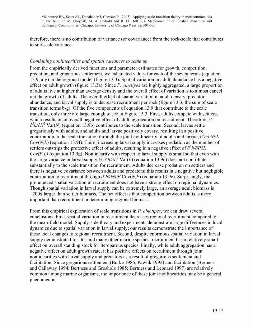
Combining nonlinearities and spatial variances to scale up From the empirically derived functions and parameter estimates for growth, competition, predation, and gregarious settlement, we calculated values for each of the seven terms (equation 13.9, a-g) in the regional model (figure 13.3). Spatial variation in adult abundance has a negative effect on adult growth (figure 13.3a). Since P. cinctipes are highly aggregated, a large proportion of adults live at higher than average density and the overall effect of variation is to almost cancel out the growth of adults. The overall effect of spatial variation in adult density, predator abundance, and larval supply is to decrease recruitment per rock (figure 13.3, the sum of scale transition terms b-g). Of the five components of equation 13.9 that contribute to the scale transition, only three are large enough to see in Figure 13.3. First, adults compete with settlers, which results in an overall negative effect of adult aggregation on recruitment. Therefore, ½ ∂2h/∂N2 Var(N) (equation 13.9b) contributes to the scale transition. Second, larvae settle gregariously with adults, and adults and larvae positively covary, resulting in a positive contribution to the scale transition through the joint nonlinearity of adults and larvae, ∂2h/∂N∂L Cov(N,L) (equation 13.9f). Third, increasing larval supply increases predation as the number of settlers outstrips the protective effect of adults, resulting in a negative effect of ∂2h/∂P∂L Cov(P,L) (equation 13.9g). Nonlinearity with respect to larval supply is small so that even with the large variance in larval supply ½ ∂2h/∂L2 Var(L) (equation 13.9d) does not contribute substantially to the scale transition for recruitment. Adults decrease predation on settlers and there is negative covariance between adults and predators; this results in a negative but negligible contribution to recruitment through ∂2h/∂N∂P Cov(N,P) (equation 13.9e). Surprisingly, the pronounced spatial variation in recruitment does not have a strong effect on regional dynamics. Though spatial variation in larval supply can be extremely large, an average adult biomass is ~200x larger than settler biomass. The net effect is that competition between adults is more important than recruitment in determining regional biomass. From this empirical exploration of scale transitions in P. cinctipes, we can draw several conclusions. First, spatial variation in recruitment decreases regional recruitment compared to the mean-field model. Supply-side theory and experiments demonstrate large differences in local dynamics due to spatial variation in larval supply; our results demonstrate the importance of these local changes to regional recruitment. Second, despite enormous spatial variation in larval supply demonstrated for this and many other marine species, recruitment has a relatively small effect on overall standing stock for iteroparous species. Finally, while adult aggregation has a negative effect on adult growth rate, it has positive effects on recruitment through joint nonlinearities with larval supply and predators as a result of gregarious settlement and facilitation. Since gregarious settlement (Burke 1986; Pawlik 1992) and facilitation (Bertness and Callaway 1994; Bertness and Grosholz 1985; Bertness and Leonard 1997) are relatively common among marine organisms, the importance of these joint nonlinearities may be a general phenomenon.


13.13

Example 3: competition between two species of annual plants The final field example is for competition between two species of annual plants. The aim was to quantify processes contributing to the coexistence of annual plants in the Chihuahuan desert, Arizona (Sears 2004). In this system, we envisage two important spatial scales: the scale of local communities, corresponding in size to the competition neighborhood of the plants, and the scale of the metacommunity where local communities are linked by dispersal of seed. The spatial scale of the metacommunity is perhaps the most natural one for examining coexistence processes, because net population dynamics at the metacommunity scale will reflect spatial variation in density and in the abiotic environment. However, the importance of metacommunity processes in providing opportunities for species coexistence, such as competition/colonization trade-offs and environmental heterogeneity, have been difficult to test, given the complexity of natural systems. Here we show how community models can be designed to be parameterized with readily available field data to quantify an important metacommunity process contributing to coexistence, the spatial storage effect (Chesson et al., chapter 12). We compared the contribution of local-scale and metacommunity-scale processes to species coexistence by comparing the effects of local competition with the influence of the spatial storage effect. The focal species were Erodium cicutarium and Phacelia popeii (hereafter Erodium and Phacelia), rosette-forming annual plants, that germinate with the winter rains, and complete their lifecycle in the spring. In the years immediately before this study, the population of Erodium, a non-native, went from low abundance at the study site to being the dominant winter annual species. Phacelia is native to the region, and has highly variable abundance depending on rainfall. Though sparse, Phacelia was the second most common annual plant during the course of the study. The spatial storage effect can arise when there is spatial environmental variation, each species has a particular patch type that is most favorable to it, (i.e. each species has an environmental niche), and species disperse between locations. If a species has a positive covariance between the favorability of the environment and the competition that it experiences at different locations, variation in the environment acts to reduce the population growth rate of the species at the metacommunity scale (Chesson 2000). When the growth rates of high density species are more limited by this mechanism than are the growth rates of low density species, then variation in the environment acts to promote coexistence. Many studies have shown that competition intensity changes with variation in the environment (see review in Goldberg et al. 1999). But when does environmental variation make a difference for community dynamics? Using carefully designed models, we can make progress in understanding how metacommunity processes contribute to diversity maintenance in complex environments.

Model to scale up the dynamics of annual plants In chapter 12, we formulated a model for the local dynamics of an annual plant community and scaled that model up to give the dynamics of the metacommunity. In that model, we saw that the dynamics of the metacommunity depend on a number of spatial covariances (Chesson et al., chapter 12, equation 12.23). Sears (2004), focuses in on one component of that model, the effect of spatial variation on plant yield and how this contributes to species coexistence through the


13.14

spatial storage effect. The spatial storage effect involves Cov(E,C), the covariance of a species’ response to the environment, E, and response to competition, C (Chesson et al., chapter 12, equation 12.26). We begin by formulating a local model for plant yield (quantified in the field as the number of inflorescences produced per adult, a surrogate for seed production), which is the result of two local processes, the response of the plant to the local environment and the response of the plant to the presence of conspecific or interspecific neighbors. In this case, the driver of the plant environmental response is the vigor (Vj) parameter described in Chesson et al. (chapter 12, Table 12.1). We use the symbol Yjx as the final yield combining vigor (V) with the yield per unit biomass (Y) and competition (C) of chapter 12 (Table 12.1). To facilitate data analysis and improve the numerical accuracy of the approximations we use a log scale. The model is defined in chapter 12 in the way most conducive to understanding, but the log scale works better for data analysis and numerical calculations. Thus, we write the yield for species j at each location x as

jxjxjx CEY −=ln , (13.10)

where Ejx is the log yield (as growth or fecundity) of an individual in response to environmental conditions alone, and Cjx is the competitive effect of neighbors on focal plants, defined as the reduction in log yield. Thus, Ejx is the log of the product of the vigor and yield per unit biomass parameters of chapter 12, and Cjx is the log of the C of chapter 12. While we generally define Cjx as a competition term, there is no sign restriction, and thus the theory permits facilitation when Cjx is negative. Yield is the anti-log of equation 13.10,

( ) jxjxjxjx CECEjx eeeY −− == . (13.11)

Thus, equation 13.11 is our local model for plant yield. To scale up from local community dynamics to the regional scale of the metacommunity, where locations are now linked by dispersal of seed, we take the spatial average of the local dynamics over all locations. We expect both the environmental response E and competition C to vary in space, so averaging over both sides of equation 13.11, and expanding the average of the product (chapter 12, equation 12.B2.6), the regional yield is

( )jjjjjj CECECEj eeeeeeY −−− +== ,Cov . (13.12)

This equation gives the exact yield for the metacommunity scale. Approximating jEe and jCe− of the mean terms as second order Taylor polynomials (chapter 12, equation 12.B2.5), and taking a linear approximation for jEe and jCe− in the covariance term (chapter 12, equation 12.B2.8) we get

( )( ) ( )( ) ( ) ( )jjCE

jCC

jEE

j CEeCeeEeeY jjjjjj ,CovVarVar 21

21 −−− −++= , (13.13)

where Var(Ej) is the spatial variance of the environmental response and Var(Cj) is the spatial variance of the competitive response. We use equation 13.13 for analyses but a more intuitive form is obtained by expanding the products and dropping a higher order term:

( ) ( ) ( ) ( ) ( ) ( ) ( )444 3444 2144 344 2144 344 21321

cb

21

a

21

modelfieldmean

,CovVarVar jjCE

jCE

jCECE

j CEeCeEeeY jjjjjjjj −−−

−

− −++= . (13.14)


13.15

Like the regional models of the previous examples, the structure of this model tells us how plant response to competition is modified at the metacommunity scale and it tells us what we need to measure in field studies to quantify the importance of metacommunity-scale processes. The dynamics of the metacommunity are given by the mean field model, which represents the average local response of each species to environment and competition, plus terms (a-c) that correct the mean field model to account for the metacommunity structure. Thus, spatial variation potentially plays an important role in the metacommunity. In addition to local responses (represented by the mean-field model), average per capita yield for each species depends on spatial variation in its response to the environment (a) and to competition (b) and on the spatial covariance of its response to environment and competition (c). Equation 13.14 tells us that spatial variance in response to the environment and competition increases the average local response to the environment, but that a positive covariance between these responses reduces a species’ yield at the metacommunity scale. However, of most interest here is how these quantities change with relative abundance of the species for then we can determine how they contribute to species coexistence (Chesson et al., chapter 12). The most important effects come from the behavior of Cov(E,C). At a metacommunity-scale, Cov(E,C) can provide a brake to population growth rates that is, in a sense, independent of local processes that promote coexistence (such as resource partitioning). Positive Cov(E,C) means that the response of a species to competition is greatest where the environment is most favorable. To promote coexistence between species, the numerically dominant competitor must have a greater positive Cov(E,C) than that of the low density species. We expect that high density species may often have a greater Cov(E,C) than low density species because they are likely to experience intense intraspecific competition in their most favorable locations in the environment. When there are species-specific differences in environmental preference, low density species are more likely than high density species to experience competitive release in their best growing locations, and for low density species there is never likely to be a strong relationship between competition intensity and the favorability of the environment (see chapter 12 for a comprehensive discussion of how this works for different types of spatial environmental variation). There are a number of reasons why it is essential to think of Cov(E,C) as an independent, emergent process. In the first place, Cov(E,C) requires environmental heterogeneity, and thus cannot be considered at small spatial scales. The effects of Cov(E,C) are also somewhat independent of neighborhood-scale resource partitioning, such as light-nutrient limitation differences or differences in rooting depth. While resource partitioning at the neighborhood scale can promote coexistence in the absence of environmental variation, likewise Cov(E,C) can promote coexistence when the relative intensity of intraspecific and interspecific neighborhood competition predicts competitive exclusion, as we show here. Finally, it is convenient to think of it as an independent mechanism because it occupies a separate position in population models, allowing us to analyze how this interaction contributes independently to coexistence. In this form, local competition intensity and Cov(E,C) are community-level parameters, allowing comparison between species, and between systems.


13.16

If a metacommunity structure is important in explaining the regional dynamics in this system, such as in promoting the coexistence of Erodium and Phacelia, then we should be able to detect and quantify the variation-dependent terms of equation 13.14 (a-c) in the field, in addition to the local response (the mean-field model) of each species in the community.

Measuring nonlinearities in annual plants In contrast to the previous two field examples, the nonlinearities here have been defined explicitly instead of being expressed as general functions. That is, yield is a nonlinear function of environment and competition (equation 13.11). As a result of these nonlinearities, the quantities to measure (equation 13.14) are Ej and Cj. Sears (2004) used a field experiment to quantify these terms. Metacommunity dynamics were estimated within a 400 m2 field site in the Chihuahuan desert of Arizona. Here, we envisage local-scale communities in 1 m2 quadrats, linked by dispersal to make up the metacommunity at the 400 m2 site scale. This habitat was dominated by Erodium, but included a sparse distribution of Phacelia and negligible densities of other annual species. A standard neighborhood competition experiment was used to compare the yield of Erodium and Phacelia with and without Erodium competitors. The experiment did not look at the intraspecific competition of Phacelia, or at its effects on Erodium, because Phacelia was at very low densities and unlikely to have strong neighborhood effects. The experiment was done in a randomized block design, where in each of ten, 1 m2 blocks distributed across the study site, two paired Erodium and two paired Phacelia plants were chosen to represent responses to the local (block) conditions. Plants in each pair were randomly assigned to removal or control treatments, where immediate neighbors were either removed or retained. The plant response to the environment (Ej) is estimated as the ln-transformed yield of plants in the removal treatment, ln(Yj,removal), thus favorable environments for either species were those blocks in which they had the most positive response in the absence of neighbors. The response to competition (Cj) is estimated as the log response-ratio of plants in the removal and control treatments, ln(Yj,removal / Yj,control). The relevant nonlinearities (equation 13.14) are derived from corrected values of Ej and Cj, described below. Local-scale competition was estimated as the mean-field response to neighbors (equation 13.14), which excludes the effects of variation in Ej or Cj.

Measuring spatial variances and covariances In previous examples, variances and covariances involved densities, that are straightforward to measure directly. Here, these quantities are measured in a field experiment by assaying the responses of individual plants to the presence and absence of neighbors. With this approach, there is no independent estimate of response to the environment and response to competition, because competitive response is estimated as the log response ratio of plants in the removal and control treatments. Thus, to accurately estimate the variances and covariance, we must correct our estimates of Ej and Cj to remove their common error. This requires a customized approach (Sears 2004; Chesson and Sears, in prep.). In this approach, the statistical model assumes that the environmental response varies between blocks within the metacommunity, but that plants of the


13.17

same species within a block (the local community) share a common environmental response. The statistical model simultaneously estimates Ej, Cj, Var(Ej), Var(Cj) and Cov(Ej, Cj).

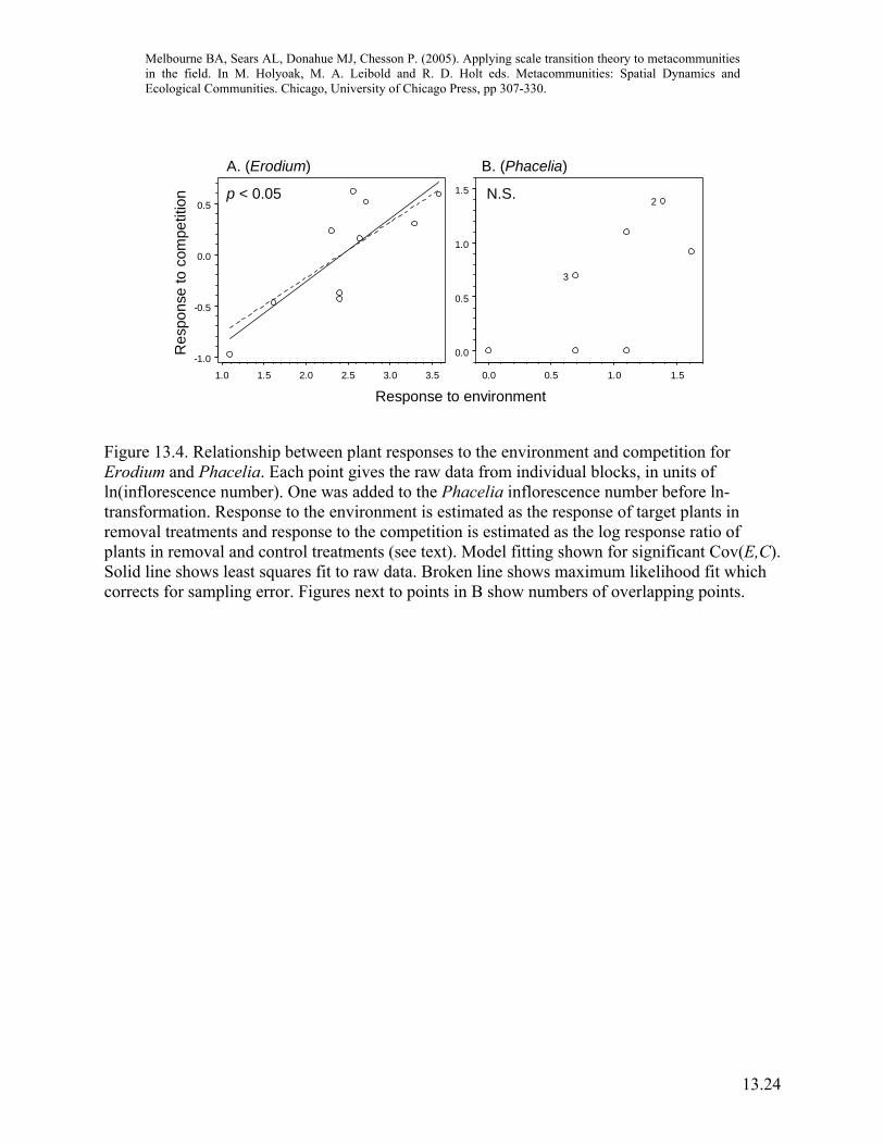
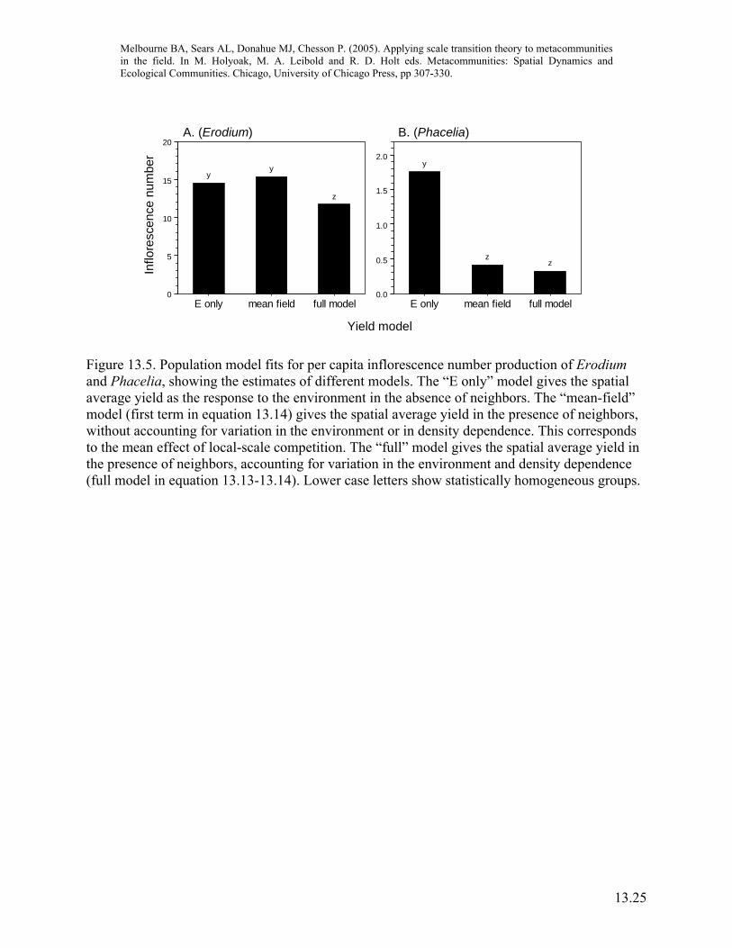
Combining the model with field data to scale up With measurements for the nonlinear function for yield and estimates of spatial variances and covariances in hand, we can now scale up the dynamics for yield from the local scale of the competition neighborhood to the scale of the metacommunity. Here we are not simply interested in the difference of the mean-field model compared to the spatial model but also in the magnitude of the different scale transition components for the two species (equation 13.14), since the relative magnitude of these components determines the importance of the spatial storage effect. For inflorescence number, Erodium had a significant positive Cov(E,C), but did not have significant local-scale intraspecific competition (Figures 13.4A, 13.5A). Figure 13.4A indicates that the lack of local scale competition was due to a balance between facilitation in poor environments, and competition in favorable environments, which in turn contributed to the positive Cov(E,C). In contrast, Phacelia experienced intense interspecific competition from Erodium, but did not have a significant Cov(E,C) (Figures 13.4B, 13.5B). Thus, covariance between plant response to the environment and competition, a process occurring only at the scale of the metacommunity, retarded the population growth rate of the dominant competitor, Erodium, while local-scale processes did not. While this study did not show that Erodium and Phacelia will continue to coexist, it demonstrates that, through the spatial storage effect, variation in the environment contributes to the possibility of coexistence, and is therefore important for metacommunity dynamics. Additionally, this study only narrowly considered the spatial storage effect as expressed through one measure of plant yield (inflorescence number). Other forms of environmental response, leading (for example) to variation in survival or germination, will have separate, contributions to the spatial storage effect and potentially provide other avenues for coexistence (Chesson et al., chapter 12). The metacommunity approach described here contrasts with traditional ANOVA tests of neighborhood competition experiments, which contain the inherent assumption that the environment is uniform because the test compares mean plant responses and does not include the effects of variance. This traditional approach, which corresponds here to the mean-field model, has two problems if we are evaluating competition in a variable environment. First, it does not include the response-enhancing effects of variance (equation 13.14). Second, and most importantly, it does not take into account the effects of Cov(E,C) which may either enhance or retard plant response at the metacommunity scale, depending on the sign of the covariance (equation 13.14). Thus, coexistence predictions from traditional neighborhood competition experiments cannot be scaled up to the metacommunity. However, ANOVA tests can be used to test whether the local-scale effects of competition are significant.

Conclusions In the three examples above, we have demonstrated the concepts and properties of the scale transition in translating the effects of local scale processes to the scale of the metacommunity.


13.18

Although concerning different field systems and different processes, the examples share a common three step approach to studying the scale transition: derive a model to scale up, measure nonlinearities, and measure spatial variances and covariances. In each example, the scale transition model identifies the important component mechanisms that change dynamics at the metacommunity scale. The structure of the model for the metacommunity scale is the same in each example, consisting of a mean-field model representing local dynamics modified by new terms to correct for spatial structure. The new terms in each model all represent interactions between nonlinearity and spatial variation. These correction terms, which can be thought of as representing spatial mechanisms, were then quantified by applying standard field experiments and sampling designs. In each example, local nonlinearities were estimated by varying levels of the nonlinear factors in an experiment and fitting models to describe the shape of the nonlinearities. Variances and covariances were measured using standard ANOVA or custom maximum likelihood procedures. In each example components of the scale transition with large magnitude were detected, confirming that metacommunity processes were, or had potential to be, important to the dynamics of the system at the larger scale.


13.19

Literature Cited Addicott, J. F., J. M. Aho, M. F. Antolin, D. K. Padilla, J. S. Richardson, and D. A. Soluk. 1987.

Ecological neighborhoods: scaling environmental patterns. Oikos 49:340-346. Armsworth, P. R. 2002. Recruitment limitation, population regulation, and larval connectivity in

reef fish metapopulations. Ecology 83:1092-1104. Bertness, M. D., and R. Callaway. 1994. Positive interactions in communities. Trends in Ecology

& Evolution 9:191-193. Bertness, M. D., and E. Grosholz. 1985. Population dynamics of the ribbed mussel, Geukensia

demissa: the costs and benefits of an aggregated distribution. Oecologia 67:192-204. Bertness, M. D., and G. H. Leonard. 1997. The role of positive interactions in communities:

Lessons from intertidal habitats. Ecology 78:1976-1989. Bolker, B., and S. W. Pacala. 1997. Using moment equations to understand stochastically driven

spatial pattern formation in ecological systems. Theoretical Population Biology 52:179-197.

Burke, R. D. 1986. Pheromones and the gregarious settlement of marine invertebrate larvae. Bulletin of Marine Science 39:323-331.

Chesson, P. 1996. Matters of scale in the dynamics of populations and communities, Pages 353-368 in R. B. Floyd, A. W. Sheppard, and P. J. De Barro, eds. Frontiers of Population Ecology. Melbourne, CSIRO Publishing.

—. 1998a. Making sense of spatial models in ecology, Pages 151-166 in J. Bascompte, and R. V. Solé, eds. Modeling Spatiotemporal Dynamics in Ecology. Austin, Landes Bioscience.

—. 1998b. Recruitment limitation: a theoretical perspective. Australian Journal of Ecology 23:234-240.

—. 2000. General theory of competitive coexistence in spatially-varying environments. Theoretical Population Biology 58:211-237.

Cooper, S. D., L. Barmuta, O. Sarnelle, K. Kratz, and S. Diehl. 1997. Quantifying spatial heterogeneity in streams. Journal of the North American Benthological Society 16:174-188.

Cooper, S. D., S. Diehl, K. Kratz, and O. Sarnelle. 1998. Implications of scale for patterns and processes in stream ecology. Australian Journal of Ecology 23:27-40.

De Jong, G. 1979. The influence of the distribution of juveniles over patches of food on the dynamics of a population. Netherlands Journal of Zoology 29:33-51.

Donahue, M. J. 2003. The interaction of dispersal and density dependence: resource variation, competition, and gregarious settlement. PhD Dissertation thesis, University of California, Davis, Davis, California.

—. 2004. Size-dependent competition in a gregarious porcelain crab, Petrolisthes cinctipes Randall (Anomura:Porcellanidae). Marine Ecology Progress Series 267:195-207.

Downes, B. J., P. S. Lake, and E. S. G. Schreiber. 1993. Spatial variation in the distribution of stream invertebrates: implications of patchiness for models of community organization. Freshwater Biology 30:119-132.

Gaines, S. D., and J. Roughgarden. 1985. Larval settlement rate: a leading determinant of structure in an ecological community of the marine intertidal zone. Proceedings of the National Academy of Sciences 82:3707-3711.


13.20

Goldberg, D. E., T. Rajaniemi, J. Gurevitch, and A. Stewart-Oaten. 1999. Empirical approaches to quantifying interaction intensity: Competition and facilitation along productivity gradients. Ecology 80:1118-1131.

Grosberg, R. K., and D. R. Levitan. 1992. For adults only? Supply-side ecology and the history of larval biology. Trends in Ecology and Evolution 7:130-133.

Hassell, M. P., R. M. May, S. W. Pacala, and P. L. Chesson. 1991. The persistence of host-parasitoid associations in patchy environments. 1. A general criterion. The American Naturalist 138:568-583.

Ives, A. R. 1988. Covariance, coexistence and the population dynamics of two competitors using a patchy resource. Journal of Theoretical Biology 133:345-361.

Jensen, G. C. 1989. Gregarious settlement by megalopae of the porcelain crabs Petrolisthes cinctipes (Randall) and Petrolisthes eriomerus (Stimpson). Journal of Experimental Marine Biology and Ecology 131:223-232.

—. 1991. Competency, settling behavior, and postsettlement aggregation by porcelain crab megalopae (Anomura: Porcellanidae). Journal of Experimental Marine Biology and Ecology 153:49-62.

Jones, G. P., M. J. Milicich, M. J. Emslie, and C. Lunow. 1999. Self-recruitment in a coral reef fish population. Nature (London) 402:802-804.

Melbourne, B. A., and P. Chesson. Submitted. The scale transition: Scaling up population dynamics with field data.

Nisbet, R. M., S. Diehl, W. G. Wilson, S. D. Cooper, D. D. Donalson, and K. Kratz. 1997. Primary-productivity gradients and short-term population dynamics in open systems. Ecological Monographs 67:535-553.

Pacala, S. W., and S. A. Levin. 1997. Biologically generated spatial pattern and the coexistence of competing species, Pages 204-232 in D. Tilman, and P. Kareiva, eds. Spatial Ecology: The Role of Space in Population Dynamics and Interspecific Interactions. Princeton, New Jersey, Princeton University Press.

Pawlik, J. R. 1992. Chemical ecology of the settlement of benthic marine invertebrates. Oceanography and Marine Biology Annual Review 30:273-335.

Searle, S. R., G. Casella, and C. E. McCulloch. 1992, Variance Components. New York, John Wiley and Sons.

Swearer, S. E., J. E. Caselle, D. W. Lea, and R. R. Warner. 1999. Larval retention and recruitment in an island population of a coral-reef fish. Nature 402:799-802.

Swearer, S. E., J. S. Shima, M. E. Hellberg, S. R. Thorrold, G. P. Jones, D. R. Robertson, S. G. Morgan et al. 2002. Evidence of self-recruitment in demersal marine populations. Bulletin of Marine Science 70:251-271.

Thorrold, S. R., G. P. Jones, M. E. Hellberg, R. S. Burton, S. E. Swearer, J. E. Neigel, S. G. Morgan et al. 2002. Quantifying larval retention and connectivity in marine populations with artificial and natural markers. Bulletin of Marine Science 70:291-308.

Underwood, A. J., and M. G. Chapman. 1996. Scales of spatial patterns of distribution of intertidal invertebrates. Oecologia 107:212-224.


13.21

( )2cm μg −A

dtAd

a b c

KΔ∗ΔA

Patch Stream

0 150 300 450-2

0

2

4

6

0 300 600 900

0

10

20

0 300 600 900

Figure 13.1. Comparison of the patch-scale model (mean-field model) and the stream-scale model for the algae-grazer system (equation 13.6). The calculations are based on fitted functions, parameter estimates, and spatial variances and covariances from field data. The shaded areas represent the reduction in the instantaneous rate of change that occurs in the stream-scale model. a) Logistic algal growth, g(A). ΔK change in carrying capacity in the logistic model. Since the logistic is quadratic, the stream-scale model is exact. b) Type III grazer removal rate, f(A)G. Dashed line is the exact stream-scale model. The dotted line is the quadratic approximation for the stream-scale model and deviates markedly from the exact model. c) Full periphyton-grazer model, g(A) - f(A)G. The stream-scale model is exact. ∗ΔA change in equilibrium biomass.


13.22

-60 -40 -20 0 20 40

oncontributiPercent

( ) ( )AAg Var21 ′′

( ) ( )AAf Var21 ′′−

( ) ( )GAAf ,Cov′−

a)

b)

c)

Figure 13.2. Contribution of each scale transition term to the total change in the equilibrium density of algae at the stream scale (equation 13.6, a-c). The calculations are based on fitted functions, parameter estimates, and spatial variances and covariances from field data. Term (a) reduced the equilibrium biomass at the stream scale and was responsible for about 60% of the total change, whereas term (b) counteracted the effect of term (a), and term (c) was of little importance. Although the terms are labeled by their quadratic approximations, the exact scale transition is shown for term (b) and (c). Term (a) is also exact, since g(A) is the logistic model and is quadratic.


13.23

-0.2 -0.1 0.0 0.1 0.2

Proportional Change in Density

(a)

(b)

(d)

(e)

(f)

(g)( )LPLP

h ,Cov2

∂∂∂

( )LLh Var

21

2

2

∂∂

( )Ng

( )LPNh ,,

( )PNPN

h ,Cov2

∂∂∂

( )LNLN

h ,Cov2

∂∂∂

( )NN

h Var21

2

2

∂∂

( )NN

g Var21

2

2

∂∂

Figure 13.3. Scale Transition for P. cinctipes. The scale transition terms (equation 13.9 a-g) are shown in gray and the mean-field model components in black. The calculations are based on fitted functions, parameter estimates, and spatial variances and covariances from field and laboratory data. All components are densities (biomass per rock) relative to the regional mean. Therefore, adult growth in the mean-field model is an increase of 24%, which is cancelled out by the scale transition for growth (a). Overall, the scale transition terms for recruitment (b-g) reduce recruitment at the regional scale compared to the mean-field model for recruitment.


13.24

0.0 0.5 1.0 1.5

0.0

0.5

1.0

1.52

3

1.0 1.5 2.0 2.5 3.0 3.5

-1.0

-0.5

0.0

0.5p < 0.05 N.S.

Response to environment

Res

pons

e to

com

petit

ion

A. (Erodium) B. (Phacelia)

Figure 13.4. Relationship between plant responses to the environment and competition for Erodium and Phacelia. Each point gives the raw data from individual blocks, in units of ln(inflorescence number). One was added to the Phacelia inflorescence number before ln-transformation. Response to the environment is estimated as the response of target plants in removal treatments and response to the competition is estimated as the log response ratio of plants in removal and control treatments (see text). Model fitting shown for significant Cov(E,C). Solid line shows least squares fit to raw data. Broken line shows maximum likelihood fit which corrects for sampling error. Figures next to points in B show numbers of overlapping points.


13.25

E only mean field full model0

5

10

15

20

yy

z

E only mean field full model0.0

0.5

1.0

1.5

2.0y

zz

Yield model

Inflo

resc

ence

num

ber

A. (Erodium) B. (Phacelia)

Figure 13.5. Population model fits for per capita inflorescence number production of Erodium and Phacelia, showing the estimates of different models. The “E only” model gives the spatial average yield as the response to the environment in the absence of neighbors. The “mean-field” model (first term in equation 13.14) gives the spatial average yield in the presence of neighbors, without accounting for variation in the environment or in density dependence. This corresponds to the mean effect of local-scale competition. The “full” model gives the spatial average yield in the presence of neighbors, accounting for variation in the environment and density dependence (full model in equation 13.13-13.14). Lower case letters show statistically homogeneous groups.

Documents

Chapter 13: Applying scale transition theory to metacommunities in