3/26/2018

1

Chapter 12/11

Part 1

Aggregate Demand II:

Applying the IS-LM Model

Goals

use the IS-LM model to analyze the effects of

shocks, fiscal policy, monetary policy affect

income and the interest rate in the short run when

prices are fixed

derive the aggregate demand curve from the IS-

LM model

Use IS-LM for long-run analysis.

explore several explanations for the

Great Depression

1

The intersection determines

the unique combination of Y and r

that satisfies equilibrium in both markets.

The LM curve represents

money market equilibrium.

Equilibrium in the IS -LM model

The IS curve represents

equilibrium in the goods

market.

( , )M P L r Y IS

Y

r = i LM

r1

Y1

Y = C(Y – T) + I (r) + 𝑮

𝒀 = 𝑪 𝒀 − 𝑻 + 𝑰 𝒊 − 𝒆 +𝑮

3/26/2018

2

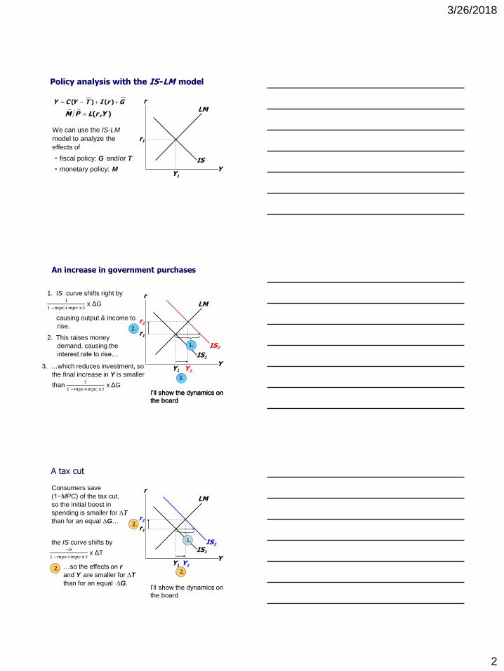
Policy analysis with the IS -LM model

We can use the IS-LM

model to analyze the

effects of

• fiscal policy: G and/or T

• monetary policy: M

Y C Y T I r G ( ) ( )

( , )M P L r Y

IS

Y

r

LM

r1

Y1

causing output & income to

rise.

IS1

An increase in government purchases

1. IS curve shifts right by 1

1 −𝑚𝑝𝑐+𝑚𝑝𝑐 x 𝑡 x ΔG

Y

r

LM

r1

Y1

IS2

Y2

r2

1.

2. This raises money

demand, causing the

interest rate to rise…

2.

3. …which reduces investment, so

the final increase in Y is smaller

than 1

1 −𝑚𝑝𝑐+𝑚𝑝𝑐 x 𝑡 x ΔG

3.

I’ll show the dynamics on

the board I’ll show the dynamics on

the board

IS1

1.

A tax cut

Y

r

LM

r1

Y1

IS2

Y2

r2

Consumers save

(1−MPC) of the tax cut,

so the initial boost in

spending is smaller for ΔT

than for an equal ΔG…

the IS curve shifts by

2.

2. …so the effects on r

and Y are smaller for ΔT

than for an equal ΔG.

2.

I’ll show the dynamics on

the board

−𝑏

1 −𝑚𝑝𝑐+𝑚𝑝𝑐 x 𝑡 x ΔT

3/26/2018

3

2. …causing the

interest rate to fall

IS

Monetary policy: An increase in M

1. ΔM > 0 shifts

the LM curve down

(or to the right)

Y

r LM1

r1

Y1 Y2

r2

LM2

3. …which increases

investment, causing

output & income to

rise.

I’ll show the dynamics on the board

r1’

1

1’

2

Slopes Matter!

If investment is inelastic, not responsive to

changes in r, IS-curve is relatively steep…

monetary policy is less effective.

But, have less crowding out, which makes fiscal

policy to be more effective.

NOW YOU TRY:

Shifting the LM curve

Suppose a wave of credit card fraud

causes consumers to use cash more

frequently in transactions.

Use the liquidity preference model

to show how these events shift the

LM curve.

3/26/2018

4

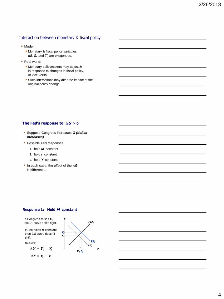
Interaction between monetary & fiscal policy

Model:

Monetary & fiscal policy variables

(M, G, and T ) are exogenous.

Real world:

Monetary policymakers may adjust M

in response to changes in fiscal policy,

or vice versa.

Such interactions may alter the impact of the

original policy change.

The Fed’s response to ΔG > 0

Suppose Congress increases G (deficit

increases).

Possible Fed responses:

1. hold M constant

2. hold r constant

3. hold Y constant

In each case, the effect of the ΔG

is different…

If Congress raises G,

the IS curve shifts right.

IS1

Response 1: Hold M constant

Y

r

LM1

r1

Y1

IS2

Y2

r2

If Fed holds M constant,

then LM curve doesn’t

shift.

Results:

2 1Y Y Y

2 1r r r

3/26/2018

5

If Congress raises G,

the IS curve shifts right.

IS1

Response 2: Hold r constant

Y

r

LM1

r1

Y1

IS2

Y2

r2

To keep r constant,

Fed increases M

to shift LM curve right.

3 1Y Y Y

0r

LM2

Y3

Results:

IS1

Response 3: Hold Y constant

Y

r

LM1

r1

IS2

Y2

r2

To keep Y constant,

Fed reduces M

to shift LM curve left.

0Y

3 1r r r

LM2

Results:

Y1

r3

If Congress raises G,

the IS curve shifts right.

Estimates of fiscal policy multipliers from the DRI macroeconometric model

Assumption about

monetary policy

Estimated

value of

Y / G

Fed holds nominal

interest rate constant

Fed holds money

supply constant

1.93

0.60

Estimated

value of

Y / T

1.19

0.26

3/26/2018

6

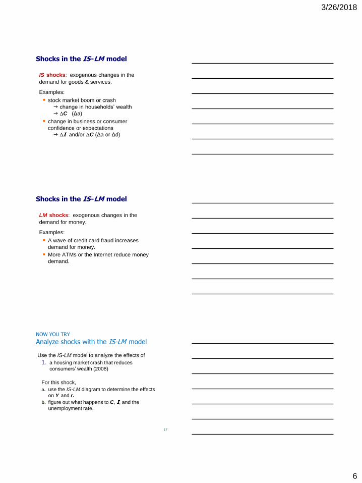
Shocks in the IS -LM model

IS shocks: exogenous changes in the

demand for goods & services.

Examples:

stock market boom or crash

g change in households’ wealth

g ΔC (Δa)

change in business or consumer

confidence or expectations

g ΔI and/or ΔC (Δa or Δd)

Shocks in the IS -LM model

LM shocks: exogenous changes in the

demand for money.

Examples:

A wave of credit card fraud increases

demand for money.

More ATMs or the Internet reduce money

demand.

NOW YOU TRY

Analyze shocks with the IS-LM model

Use the IS-LM model to analyze the effects of

1. a housing market crash that reduces

consumers’ wealth (2008)

For this shock,

a. use the IS-LM diagram to determine the effects

on Y and r.

b. figure out what happens to C, I, and the

unemployment rate.

17

3/26/2018

7

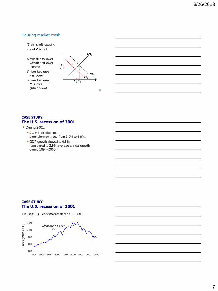
Housing market crash

18

IS1

Y

r

LM1

r1

Y1

IS2

Y2

r2

IS shifts left, causing

r and Y to fall.

C falls due to lower

wealth and lower

income,

I rises because

r is lower

u rises because

Y is lower

(Okun’s law)

CASE STUDY:

The U.S. recession of 2001

During 2001:

2.1 million jobs lost,

unemployment rose from 3.9% to 5.8%.

GDP growth slowed to 0.8%

(compared to 3.9% average annual growth

during 1994–2000).

CASE STUDY:

The U.S. recession of 2001

Causes: 1) Stock market decline g iC

300

600

900

1,200

1,500

1995 1996 1997 1998 1999 2000 2001 2002 2003

Inde

x (

194

2 =

100

)

Standard & Poor’s

500

3/26/2018

8

CASE STUDY:

The U.S. recession of 2001

Causes: 2) 9/11

increased uncertainty

fall in consumer & business confidence

result: lower spending, IS curve shifted left

Causes: 3) Corporate accounting scandals

Enron, WorldCom, etc.

reduced stock prices, discouraged investment

CASE STUDY:

The U.S. recession of 2001

Fiscal policy response: shifted IS curve right

tax cuts in 2001 and 2003

spending increases

airline industry bailout

NYC reconstruction

Afghanistan war

CASE STUDY:

The U.S. recession of 2001

Monetary policy response: shifted LM curve right

Three-month

T-Bill rate

0

1

2

3

4

5

6

7

3/26/2018

9

shocks - defined

Monetary Policy:

Decrease in i − increase in M

− monetary

expansion

Increase in i − decrease in M

− monetary

contraction − monetary tightening

Shocks - defined

Fiscal Policy:

Increase in T–G − fiscal contraction

− also

called fiscal consolidation

Decrease in T–G − fiscal expansion

What is the Fed’s policy instrument?

The news media commonly report the Fed’s policy

changes as interest rate changes, as if the Fed

has direct control over market interest rates.

In fact, the Fed targets the federal funds rate—the

interest rate banks charge one another on

overnight loans.

The Fed changes the money supply and shifts the

LM curve to achieve its target.

Other short-term rates typically move with the

federal funds rate.

3/26/2018

10

What is the Fed’s policy instrument?

Why does the Fed target interest rates instead of

the money supply?

1) They are easier to measure than the money

supply.

2) The Fed might believe that LM shocks are

more prevalent than IS shocks. If so, then

targeting the interest rate stabilizes income

better than targeting the money supply.

(See problem 8 on p.364.)

Some argue: If Fed chooses the interest rate

target and adjusts the money supply to

achieve it, draw a horizontal LM curve.

IS

LM

Y

r1

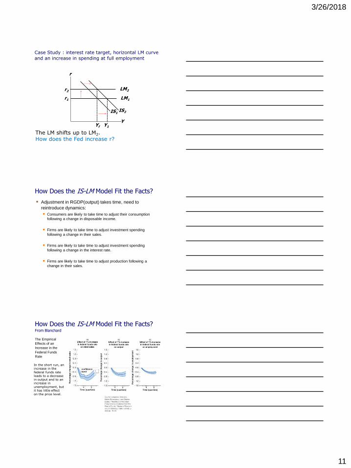
Case Study : interest rate target, horizontal LM curve

and an increase in spending at full employment

If IS2 represents a permanent increase in spending, Y1 – Yf is a positive output gap which exerts upward pressure on inflation. The Fed responds by increasing r.

IS1

LM1

Yf

r1

IS2

Y1

3/26/2018

11

Case Study : interest rate target, horizontal LM curve

and an increase in spending at full employment

The LM shifts up to LM2. How does the Fed increase r?

IS1

LM1

Yf

r1

IS2

Y1

LM2 r2

How Does the IS-LM Model Fit the Facts?

Adjustment in RGDP(output) takes time, need to

reintroduce dynamics:

Consumers are likely to take time to adjust their consumption

following a change in disposable income.

Firms are likely to take time to adjust investment spending

following a change in their sales.

Firms are likely to take time to adjust investment spending

following a change in the interest rate.

Firms are likely to take time to adjust production following a

change in their sales.

How Does the IS-LM Model Fit the Facts? From Blanchard

The Empirical

Effects of an

Increase in the

Federal Funds

Rate

In the short run, an increase in the federal funds rate leads to a decrease in output and to an increase in unemployment, but it has little effect on the price level.

3/26/2018

12

How Does the IS-LM Model Fit the Facts?

The Empirical Effects of

an Increase in the Federal

Funds Rate

IS-LM and Aggregate Demand

So far, we’ve been using the IS-LM model to

analyze the short run, when the price level is

assumed fixed.

However, a change in P would shift LM and

therefore affect Y.

The aggregate demand curve

(introduced in Chap. 10) captures this

relationship between P and Y.

Y1 Y2

Deriving the AD curve

Y

r

Y

P

IS

LM(P1)

LM(P2)

AD

P1

P2

Y2 Y1

r2

r1

Intuition for slope

of AD curve:

hP g i(M/P )

g LM shifts left

g hr

g iI

g iY

3/26/2018

13

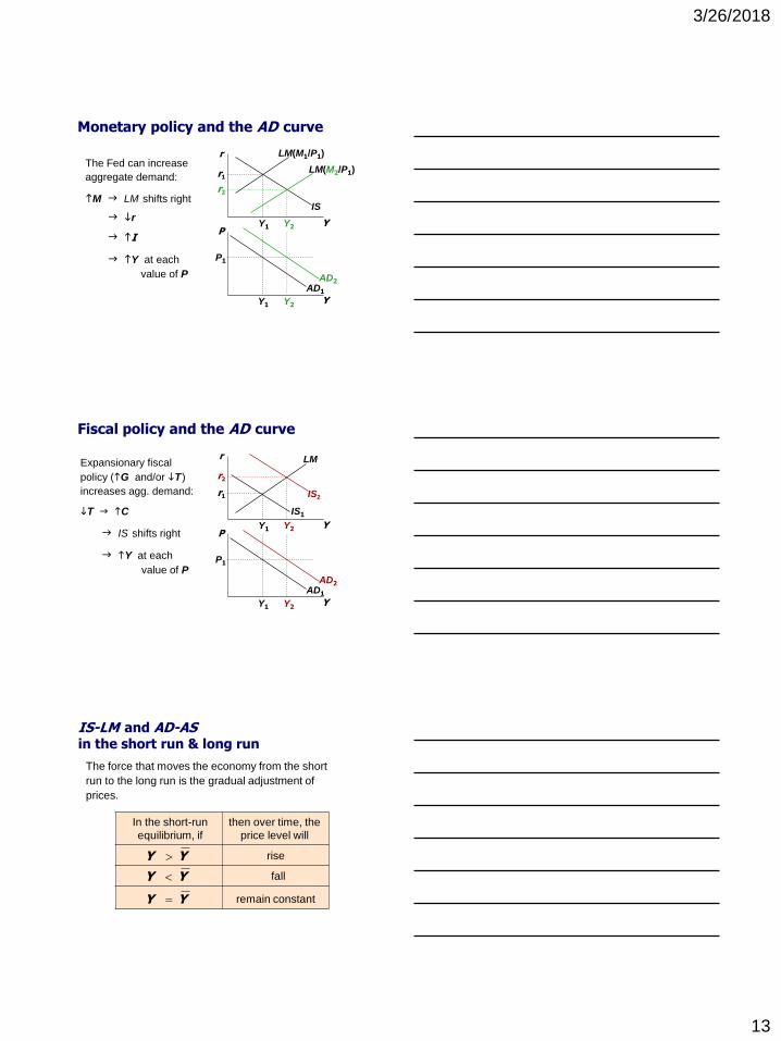
Monetary policy and the AD curve

Y

P

IS

LM(M2/P1)

LM(M1/P1)

AD1

P1

Y1

Y1

Y2

Y2

r1

r2

The Fed can increase

aggregate demand:

hM g LM shifts right

AD2

Y

r

g ir

g hI

g hY at each

value of P

Y2

Y2

r2

Y1

Y1

r1

Fiscal policy and the AD curve

Y

r

Y

P

IS1

LM

AD1

P1

Expansionary fiscal

policy (hG and/or iT )

increases agg. demand:

iT g hC

g IS shifts right

g hY at each

value of P AD2

IS2

IS-LM and AD-AS in the short run & long run

The force that moves the economy from the short

run to the long run is the gradual adjustment of

prices.

Y Y

Y Y

Y Y

rise

fall

remain constant

In the short-run

equilibrium, if

then over time, the

price level will

3/26/2018

14

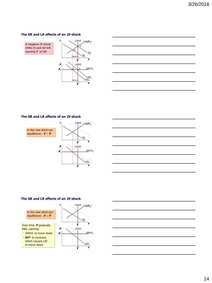
The SR and LR effects of an IS shock

A negative IS shock

shifts IS and AD left,

causing Y to fall.

Y

r

Y

P LRAS

Y

LRAS

Y

IS1

SRAS1 P1

LM(P1)

IS2

AD2

AD1

A

B

A B

The SR and LR effects of an IS shock

Y

r

Y

P LRAS

Y

LRAS

Y

IS1

SRAS1 P1

LM(P1)

IS2

AD2

AD1

In the new short-run

equilibrium, Y Y

The SR and LR effects of an IS shock

Y

r

Y

P LRAS

Y

LRAS

Y

IS1

SRAS1 P1

LM(P1)

IS2

AD2

AD1

In the new short-run

equilibrium, Y Y

Over time, P gradually

falls, causing:

• SRAS to move down

• M/P to increase,

which causes LM

to move down

3/26/2018

15

AD2

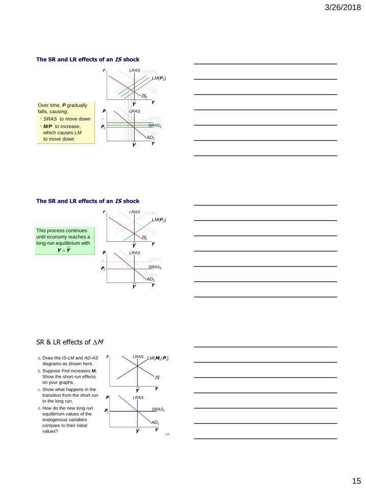
The SR and LR effects of an IS shock

Y

r

Y

P LRAS

Y

LRAS

Y

IS1

SRAS1 P1

LM(P1)

IS2

AD1

SRAS2 P2

LM(P2)

Over time, P gradually

falls, causing:

• SRAS to move down

• M/P to increase,

which causes LM

to move down

AD2

SRAS2 P2

LM(P2)

The SR and LR effects of an IS shock

Y

r

Y

P LRAS

Y

LRAS

Y

IS1

SRAS1 P1

LM(P1)

IS2

AD1

This process continues

until economy reaches a

long-run equilibrium with

Y Y

SR & LR effects of ΔM

44

a. Draw the IS-LM and AD-AS

diagrams as shown here.

b. Suppose Fed increases M.

Show the short-run effects

on your graphs.

c. Show what happens in the

transition from the short run

to the long run.

d. How do the new long-run

equilibrium values of the

endogenous variables

compare to their initial

values?

Y

r

Y

P LRAS

Y

LRAS

Y

IS

SRAS1 P1

LM(M1/P1)

AD1

3/26/2018

16

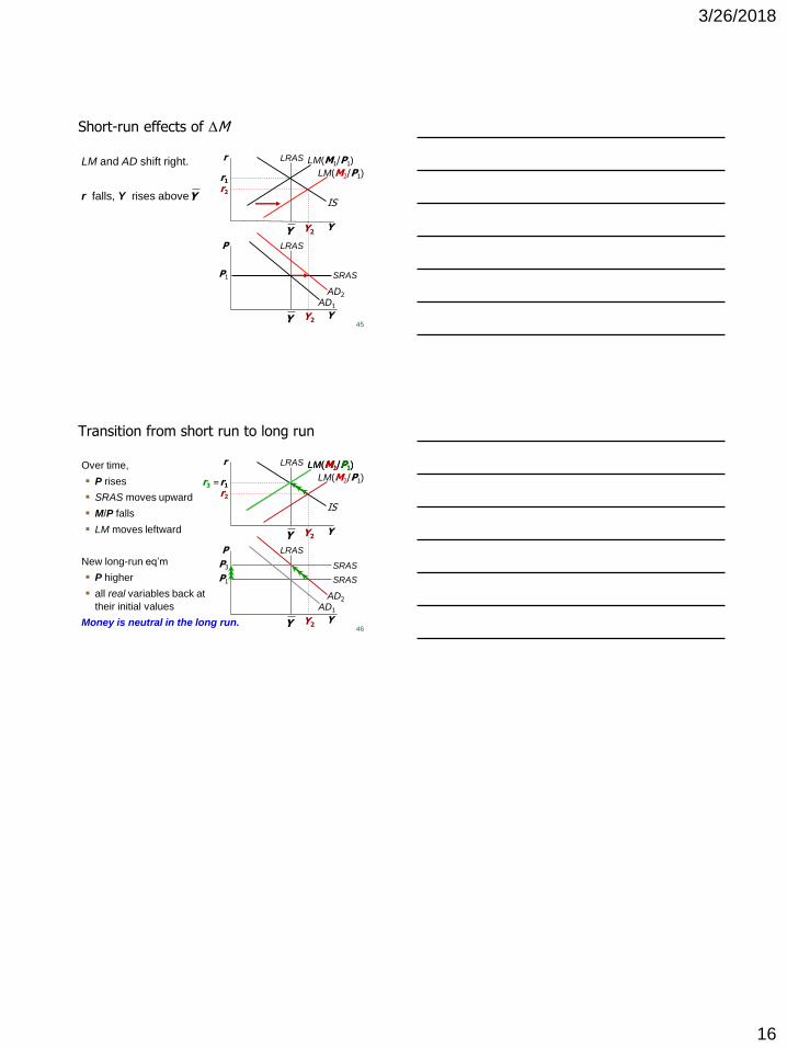
Short-run effects of ΔM

45

LM and AD shift right.

r falls, Y rises above

Y

r

Y

P LRAS

Y

LRAS

Y

IS

SRAS P1

LM(M1/P1)

AD1

LM(M2/P1)

AD2

Y2

Y2

r2

r1

Y

Transition from short run to long run

46

Over time,

P rises

SRAS moves upward

M/P falls

LM moves leftward

New long-run eq’m

P higher

all real variables back at

their initial values

Money is neutral in the long run.

Y

r

Y

P LRAS

Y

LRAS

Y

IS

SRAS P1

LM(M1/P1)

AD1

LM(M2/P1)

AD2

Y2

Y2

r2

r1

LM(M2/P3)

SRAS P3

r3 =