Embed Size (px)
Citation preview
Chapter 12
Embedding an Affine Space in aVector Space
12.1 Embedding an Affine Space as a Hyperplane in a
Vector Space: the “Hat Construction”
Assume that we consider the real affine space E of dimen-
sion 3, and that we have some affine frame (a0, (−→v1 ,−→v2 ,−→v2 )).
With respect to this affine frame, every point x ∈ E isrepresented by its coordinates (x1, x2, x3), where
a = a0 + x1−→v1 + x2
−→v2 + x3−→v3 .
A vector −→u ∈ −→E is also represented by its coordinates
(u1, u2, u3) over the basis (−→v1 ,−→v2 ,−→v2 ).
481
482 CHAPTER 12. EMBEDDING AN AFFINE SPACE IN A VECTOR SPACE
One way to distinguish between points and vectors isto add a fourth coordinate, and to agree that points arerepresented by (row) vectors (x1, x2, x3, 1) whose fourthcoordinate is 1, and that vectors are represented by (row)vectors (v1, v2, v3, 0) whose fourth coordinate is 0.
This “programming trick” works actually very well. Ofcourse, we are opening the door for strange elements suchas (x1, x2, x3, 5), where the fourth coordinate is neither 1nor 0.
12.1. THE “HAT CONSTRUCTION” 483
The question is, can we make sense of such elementsand of such a construction?
The answer is “yes”. We will present a construction in
which an affine space (E,−→E ) is embedded in a vector
space E, in which−→E is embedded as a hyperplane pass-
ing through the origin, and E itself is embedded as anaffine hyperplane, defined as ω−1(1), for some linear form
ω: E → R.
The vector space E has the universal property that for
any vector space−→F and any affine map f : E → −→
F ,
there is a unique linear map f : E → −→F extending
f : E → −→F .
484 CHAPTER 12. EMBEDDING AN AFFINE SPACE IN A VECTOR SPACE
Some Simple Geometric Transformations
Given an affine space (E,−→E ), every −→u ∈ −→
E induces amapping tu: E → E, called a translation, and defined
such that tu(a) = a + −→u , for every a ∈ E.
Clearly, the set of translations is a vector space isomorphic
to−→E .
Given any point a and any scalar λ ∈ R, we definethe mapping Ha,λ: E → E, called dilatation (or centralmagnification, or homothety) of center a and ratio λ,and defined such that
Ha,λ(x) = a + λ−→ax,
for every x ∈ E.
Ha,λ(a) = a, and when λ = 0 and x = a, Ha,λ(x) is onthe line defined by a and x, and is obtained by “scaling”−→ax by λ. The effect is a uniform dilatation (or contrac-tion, if λ < 1).
12.1. THE “HAT CONSTRUCTION” 485
When λ = 0, Ha,0(x) = a for all x ∈ E, and Ha,0 is theconstant affine map sending every point to a.
If we assume λ = 1, note that Ha,λ is never the identity,and since a is a fixed-point, Ha,λ is never a translation.
We now consider the set E of geometric transformationsfrom E to E, consisting of the union of the (disjoint) setsof translations and dilatations of ratio λ = 1.
We would like to give this set the structure of a vector
space, in such a way that both E and−→E can be natu-
rally embedded into E.
In fact, it will turn out that barycenters show up quitenaturally too!
486 CHAPTER 12. EMBEDDING AN AFFINE SPACE IN A VECTOR SPACE
In order to “add” two dilatations Ha1,λ1 and Ha2,λ2, itturns out that it is more convenient to consider dilatationsof the form Ha,1−λ, where λ = 0.
To see this, let us see the effect of such a dilatation on apoint x ∈ E: we have
Ha,1−λ(x) = a + (1 − λ)−→ax = a + −→ax − λ−→ax = x + λ−→xa.
For simplicity of notation, let us denote Ha,1−λ as 〈a, λ〉.Then, we have
〈a, λ〉(x) = x + λ−→xa.
12.1. THE “HAT CONSTRUCTION” 487
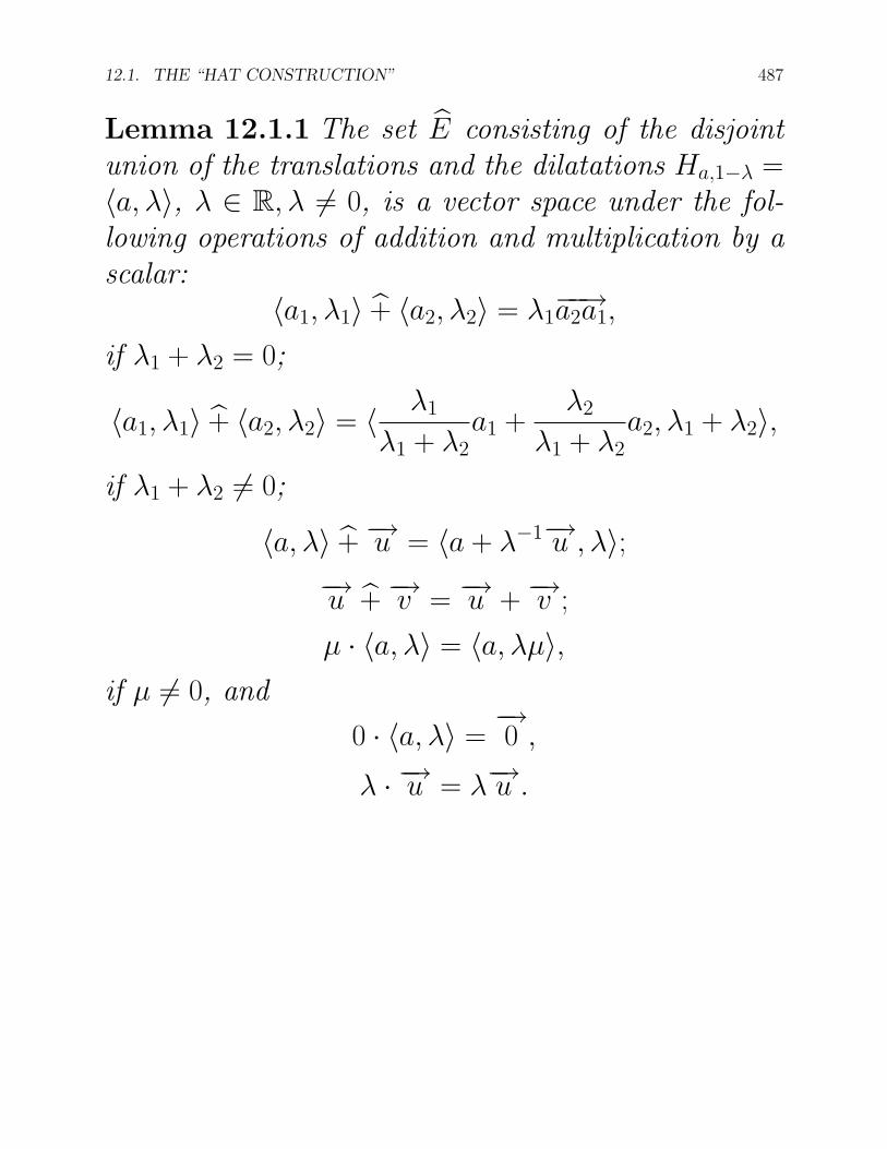
Lemma 12.1.1 The set E consisting of the disjointunion of the translations and the dilatations Ha,1−λ =〈a, λ〉, λ ∈ R, λ = 0, is a vector space under the fol-lowing operations of addition and multiplication by ascalar:
〈a1, λ1〉 + 〈a2, λ2〉 = λ1−−→a2a1,
if λ1 + λ2 = 0;
〈a1, λ1〉 + 〈a2, λ2〉 = 〈 λ1
λ1 + λ2a1 +
λ2
λ1 + λ2a2, λ1 + λ2〉,
if λ1 + λ2 = 0;
〈a, λ〉 + −→u = 〈a + λ−1−→u , λ〉;−→u + −→v = −→u + −→v ;
µ · 〈a, λ〉 = 〈a, λµ〉,if µ = 0, and
0 · 〈a, λ〉 =−→0 ,
λ · −→u = λ−→u .
488 CHAPTER 12. EMBEDDING AN AFFINE SPACE IN A VECTOR SPACE
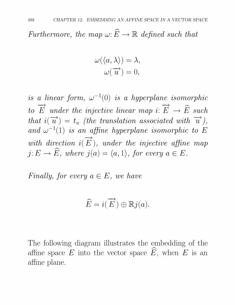
Furthermore, the map ω: E → R defined such that
ω(〈a, λ〉) = λ,
ω(−→u ) = 0,
is a linear form, ω−1(0) is a hyperplane isomorphic
to−→E under the injective linear map i:
−→E → E such
that i(−→u ) = tu (the translation associated with −→u ),and ω−1(1) is an affine hyperplane isomorphic to E
with direction i(−→E ), under the injective affine map
j: E → E, where j(a) = 〈a, 1〉, for every a ∈ E.
Finally, for every a ∈ E, we have
E = i(−→E ) ⊕ Rj(a).
The following diagram illustrates the embedding of theaffine space E into the vector space E, when E is anaffine plane.
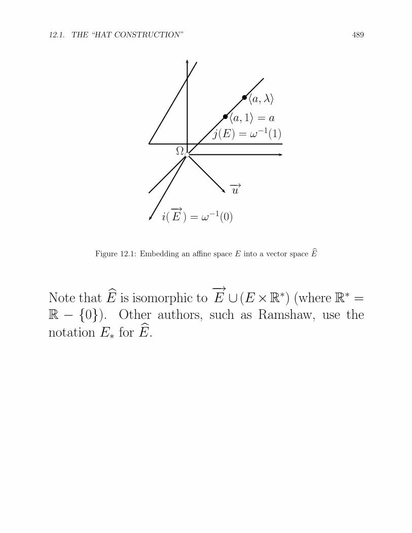
12.1. THE “HAT CONSTRUCTION” 489
Ω
〈a, 1〉 = a
〈a, λ〉
i(−→E ) = ω−1(0)
j(E) = ω−1(1)
−→u
Figure 12.1: Embedding an affine space E into a vector space E
Note that E is isomorphic to−→E ∪ (E×R
∗) (where R∗ =
R − 0). Other authors, such as Ramshaw, use the
notation E∗ for E.
490 CHAPTER 12. EMBEDDING AN AFFINE SPACE IN A VECTOR SPACE
Ramshaw calls the linear form ω: E → R a weight (or
flavor), and he says that an element z ∈ E such thatω(z) = λ is λ-heavy (or has flavor λ) ([?]).
The elements of j(E) are 1-heavy and are called points ,
and the elements of i(−→E ) are 0-heavy and are called vec-
tors .
In general, the λ-heavy elements all belong to the hyper-
plane ω−1(λ) parallel to i(−→E ).
Thus, intuitively, we can thing of E as a stack of parallelhyperplanes, one for each λ, a little bit like an infinitestack of very thin pancakes!
12.1. THE “HAT CONSTRUCTION” 491
There are two privileged pancakes: one corresponding to
E, for λ = 1, and one corresponding to−→E , for λ = 0.
From now on, we will identify j(E) and E, and i(−→E ) and
−→E .
We will also write λa instead of 〈a, λ〉, which we will calla weighted point , and write 1a just as a.
When we want to be more precise, we may also write〈a, 1〉 as a (as Ramshaw does).
492 CHAPTER 12. EMBEDDING AN AFFINE SPACE IN A VECTOR SPACE
In particular, when we consider the homogenized versionA of the affine space A associated with the base field R
considered as an affine space, we write λ for 〈λ, 1〉, when
viewing λ as a point in both A and A, and simply λ,when viewing λ as a vector in R and in A.
The elements of A are called Bezier sites , by Ramshaw.
Then, in view of the fact that
〈a + −→u , 1〉 = 〈a, 1〉 + −→u ,
and since we are identifying a +−→u with 〈a +−→u , 1〉 (un-der the injection j), in the simplified notation, the above
reads as a + −→u = a + −→u .
Thus, we go one step further, and denote a+−→u as a+−→u .
From lemma 12.1.1, for every a ∈ E, every element of E
can be written uniquely as −→u + λa.
We also denoteλa + (−µ)b
asλa − µb.
12.1. THE “HAT CONSTRUCTION” 493
Given any family (ai)i∈I of points in E, and any family(λi)i∈I of scalars in R, with finite support, it is easilyshown by induction on the size of the support of (λi)i∈I
that,
(1) If∑
i∈I λi = 0, then∑i∈I
〈ai, λi〉 =∑i∈I
λiai,
where ∑i∈I
λiai =∑i∈I
λi−→bai
for any b ∈ E, which, by lemma 2.2.1, is a vector inde-pendent of b, or
(2) If∑
i∈I λi = 0, then∑i∈I
〈ai, λi〉 = 〈∑i∈I
λi∑i∈I λi
ai,∑i∈I
λi〉.
Thus, we see how barycenters reenter the scene quitenaturally, and that in E, we can make sense of
∑i∈I〈ai, λi〉,
regardless of the value of∑
i∈I λi.
494 CHAPTER 12. EMBEDDING AN AFFINE SPACE IN A VECTOR SPACE
When∑
i∈I λi = 1, the element∑
i∈I〈ai, λi〉 belongs tothe hyperplane ω−1(1), and thus, it is a point.
When∑
i∈I λi = 0, the linear combination of points∑i∈I λiai is a vector, and when I = 1, . . . , n, we allow
ourselves to write
λ1a1 + · · · + λnan,
where some of the occurrences of + can be replaced by− , as
λ1a1 + · · · + λnan,
where the occurrences of − (if any) are replaced by −.
In fact, we have the following slightly more general prop-erty, which is left as an exercise.
12.1. THE “HAT CONSTRUCTION” 495
Lemma 12.1.2 Given any affine space (E,−→E ), for
any family (ai)i∈I of points in E, for any family (λi)i∈I
of scalars in R, with finite support, and any family
(−→vj )j∈J of vectors in−→E also with finite support, and
with I ∩ J = ∅, the following properties hold:
(1) If∑
i∈I λi = 0, then∑i∈I
〈ai, λi〉 +∑j∈J
−→vj =∑i∈I
λiai +∑j∈J
−→vj ,
where ∑i∈I
λiai =∑i∈I
λi−→bai
for any b ∈ E, which, by lemma 2.2.1, is a vectorindependent of b, or
(2) If∑
i∈I λi = 0, then∑i∈I
〈ai, λi〉 +∑j∈J
−→vj
= 〈∑i∈I
λi∑i∈I λi
ai +∑j∈J
−→vj∑i∈I λi
,∑i∈I
λi〉.
496 CHAPTER 12. EMBEDDING AN AFFINE SPACE IN A VECTOR SPACE
The above formulae show that we have some kind ofextended barycentric calculus .
Operations on weighted points and vectors were intro-duced by H. Grassmann, in his book published in 1844!This calculus is helpful in dealing with rational curves.
There is also a nice relationship between affine frames in
(E,−→E ) and bases of E, stated in the following lemma.
Lemma 12.1.3 Given any affine space (E,−→E ), for
any affine frame (a0, (−−→a0a1, . . . ,
−−→a0am)) for E, the fam-
ily (−−→a0a1, . . . ,−−→a0am, a0) is a basis for E, and for any
affine frame (a0, . . . , am) for E, the family (a0, . . . , am)
is a basis for E.
Furthermore, given any element 〈x, λ〉 ∈ E, if
x = a0 + x1−−→a0a1 + · · · + xm
−−→a0am
over the affine frame (a0, (−−→a0a1, . . . ,
−−→a0am)) in E, thenthe coordinates of 〈x, λ〉 over the basis
(−−→a0a1, . . . ,−−→a0am, a0)
in E, are(λx1, . . . , λxm, λ).
12.1. THE “HAT CONSTRUCTION” 497
For any vector −→v ∈ −→E , if
−→v = v1−−→a0a1 + · · · + vm
−−→a0am
over the basis(−−→a0a1, . . . ,
−−→a0am)
in−→E , then over the basis
(−−→a0a1, . . . ,−−→a0am, a0)
in E, the coordinates of −→v are
(v1, . . . , vm, 0).
498 CHAPTER 12. EMBEDDING AN AFFINE SPACE IN A VECTOR SPACE
For any element 〈a, λ〉, where λ = 0, if the barycentriccoordinates of a w.r.t. the affine basis (a0, . . . , am) inE are (λ0, . . . , λm) with λ0 + · · · + λm = 1, then the
coordinates of 〈a, λ〉 w.r.t. the basis (a0, . . . , am) in Eare
(λλ0, . . . , λλm).
If a vector −→v ∈ −→E is expressed as
−→v = v1−−→a0a1 + · · · + vm
−−→a0am
= −(v1 + · · · + vm)a0 + v1a1 + · · · + vmam,
with respect to the affine basis (a0, . . . , am) in E, then
its coordinates w.r.t. the basis (a0, . . . , am) in E are
(−(v1 + · · · + vm), v1, . . . , vm).
12.1. THE “HAT CONSTRUCTION” 499
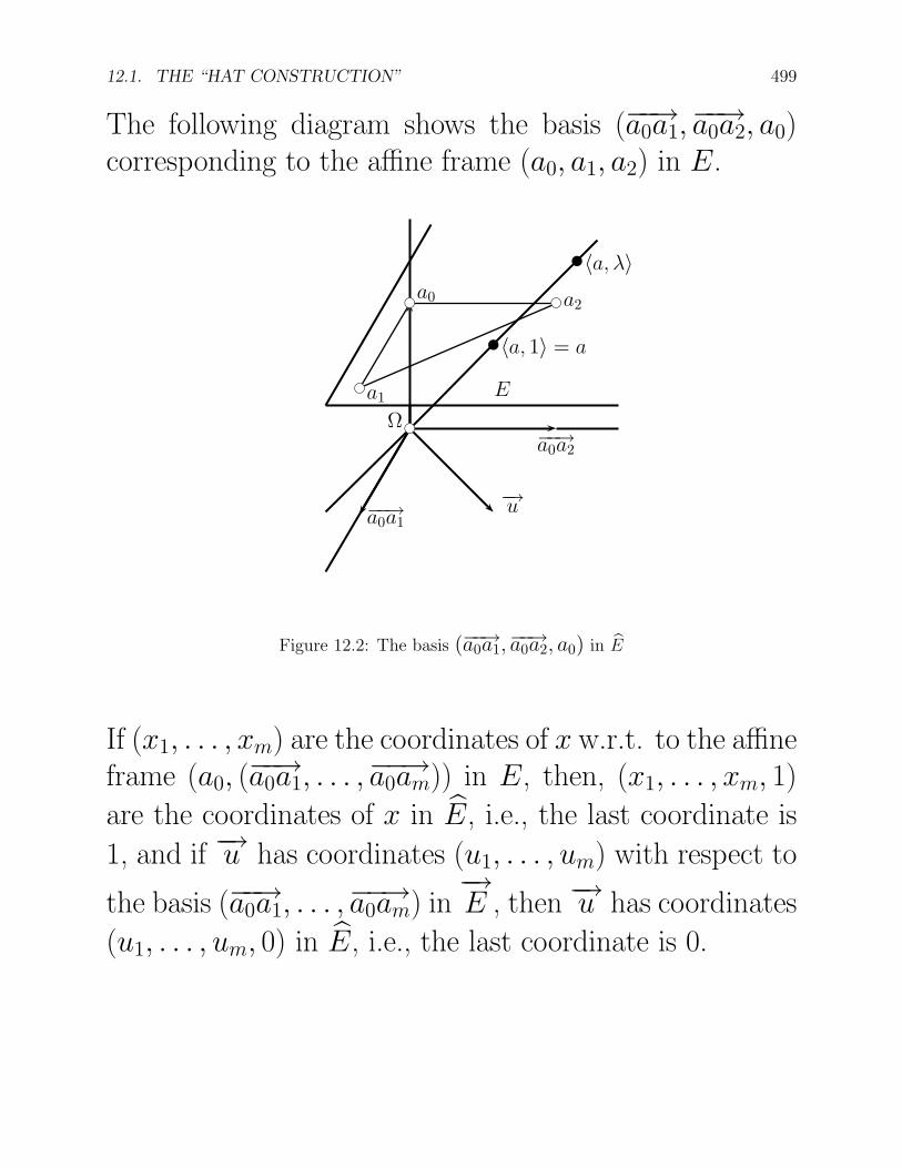
The following diagram shows the basis (−−→a0a1,−−→a0a2, a0)
corresponding to the affine frame (a0, a1, a2) in E.
Ω
〈a, 1〉 = a
〈a, λ〉
−−→a0a1
−−→a0a2
a0
a1
a2
−→u
E
Figure 12.2: The basis (−−→a0a1,−−→a0a2, a0) in E
If (x1, . . . , xm) are the coordinates of x w.r.t. to the affineframe (a0, (
−−→a0a1, . . . ,−−→a0am)) in E, then, (x1, . . . , xm, 1)
are the coordinates of x in E, i.e., the last coordinate is
1, and if −→u has coordinates (u1, . . . , um) with respect to
the basis (−−→a0a1, . . . ,−−→a0am) in
−→E , then −→u has coordinates
(u1, . . . , um, 0) in E, i.e., the last coordinate is 0.
500 CHAPTER 12. EMBEDDING AN AFFINE SPACE IN A VECTOR SPACE
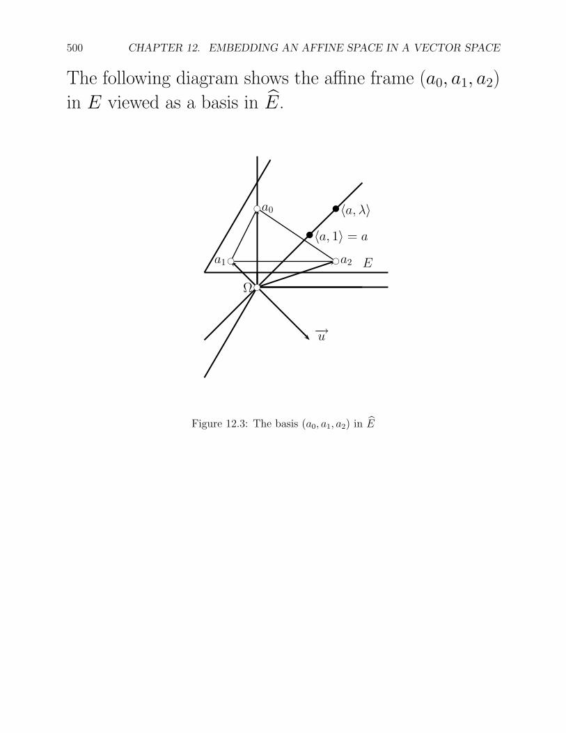
The following diagram shows the affine frame (a0, a1, a2)
in E viewed as a basis in E.
Ω
〈a, 1〉 = a
〈a, λ〉
a1 a2
a0
−→u
E
Figure 12.3: The basis (a0, a1, a2) in E
12.1. THE “HAT CONSTRUCTION” 501
Now that we have defined E and investigated the rela-tionship between affine frames in E and bases in E, wecan give one more construction of a vector space F from
E and−→E , that will allow us to “visualize” in a much more
intuitive fashion the structure of E and of its operations+ and ·.
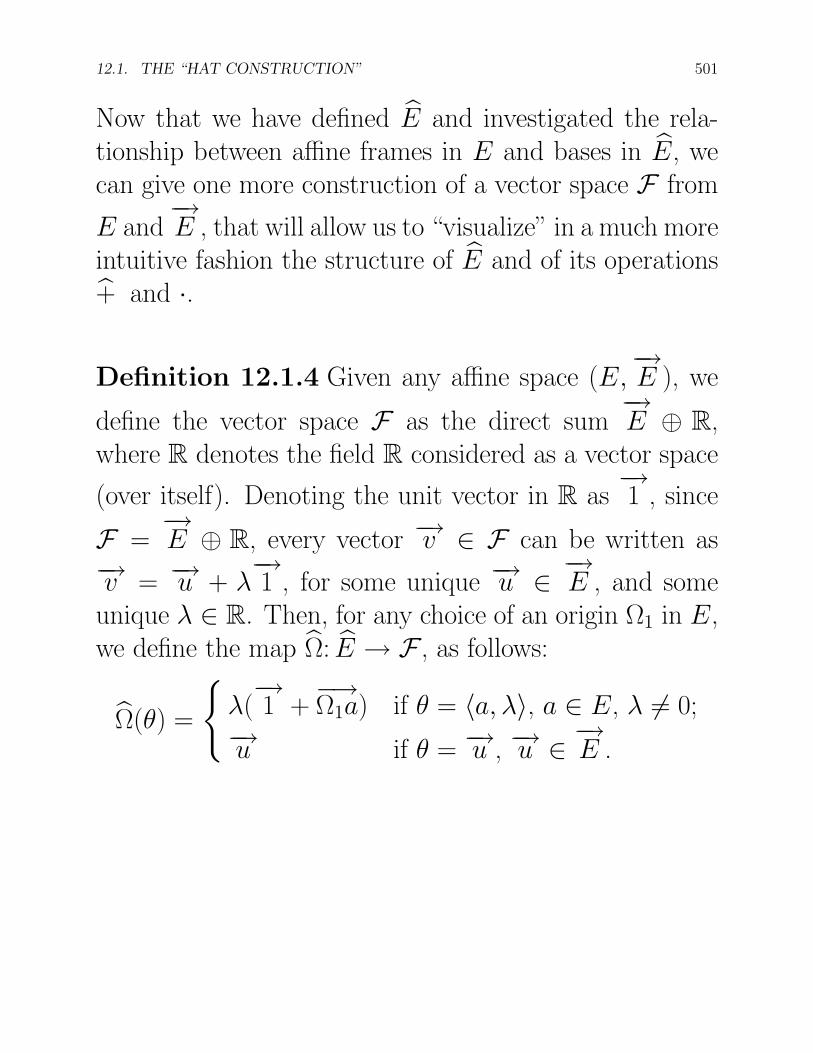
Definition 12.1.4 Given any affine space (E,−→E ), we
define the vector space F as the direct sum−→E ⊕ R,
where R denotes the field R considered as a vector space
(over itself). Denoting the unit vector in R as−→1 , since
F =−→E ⊕ R, every vector −→v ∈ F can be written as
−→v = −→u + λ−→1 , for some unique −→u ∈ −→
E , and someunique λ ∈ R. Then, for any choice of an origin Ω1 in E,we define the map Ω: E → F , as follows:
Ω(θ) =
λ(−→1 +
−→Ω1a) if θ = 〈a, λ〉, a ∈ E, λ = 0;
−→u if θ = −→u , −→u ∈ −→E .
502 CHAPTER 12. EMBEDDING AN AFFINE SPACE IN A VECTOR SPACE
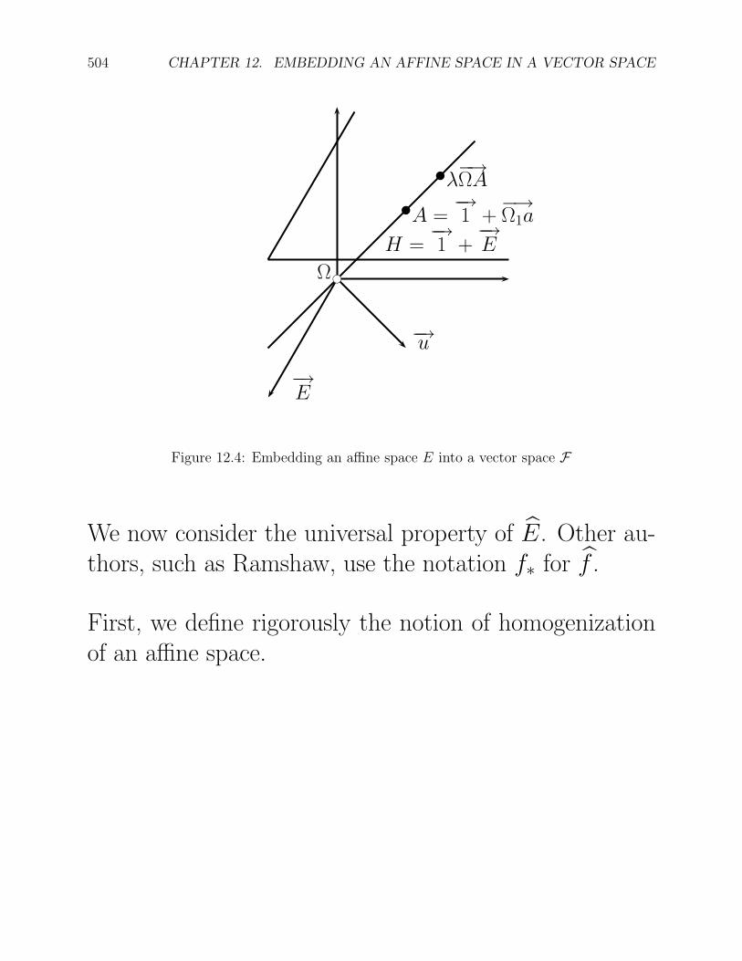
The idea is that, once again, viewing F as an affine spaceunder its canonical structure, E is embedded in F as
the hyperplane H =−→1 +
−→E , with direction
−→E , the
hyperplane−→E in F .
Then, every point a ∈ E is in bijection with the point
A =−→1 +
−→Ω1a, in the hyperplane H .
Denoting the origin−→0 of the canonical affine space F as
Ω, the map Ω maps a point 〈a, λ〉 ∈ E to a point in F , as
follows: Ω(〈a, λ〉) is the point on the line passing through
both the origin Ω of F and the point A =−→1 +
−→Ω1a in
the hyperplane H =−→1 +
−→E , such that
Ω(〈a, λ〉) = λ−→ΩA = λ(
−→1 +
−→Ω1a).
The following lemma shows that Ω is an isomorphism ofvector spaces.
12.1. THE “HAT CONSTRUCTION” 503
Lemma 12.1.5 Given any affine space (E,−→E ), for
any choice Ω1 of an origin in E, the map Ω: E → F isa linear isomorphism between E and the vector spaceF of definition 12.1.4. The inverse of Ω is given by
Ω−1(−→u + λ−→1 ) =
〈Ω1 + λ−1−→u , λ〉) if λ = 0;−→u if λ = 0.
The following diagram illustrates the embedding of theaffine space E into the vector space F , when E is anaffine plane.
504 CHAPTER 12. EMBEDDING AN AFFINE SPACE IN A VECTOR SPACE
Ω
A =−→1 +
−→Ω1a
λ−→ΩA
−→E
H =−→1 +
−→E
−→u
Figure 12.4: Embedding an affine space E into a vector space F
We now consider the universal property of E. Other au-thors, such as Ramshaw, use the notation f∗ for f .
First, we define rigorously the notion of homogenizationof an affine space.
12.1. THE “HAT CONSTRUCTION” 505
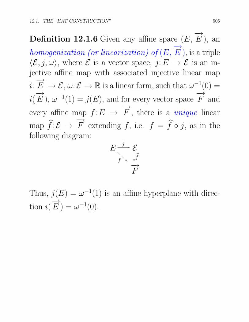
Definition 12.1.6 Given any affine space (E,−→E ), an
homogenization (or linearization) of (E,−→E ), is a triple
〈E , j, ω〉, where E is a vector space, j: E → E is an in-jective affine map with associated injective linear map
i:−→E → E , ω: E → R is a linear form, such that ω−1(0) =
i(−→E ), ω−1(1) = j(E), and for every vector space
−→F and
every affine map f : E → −→F , there is a unique linear
map f : E → −→F extending f , i.e. f = f j, as in the
following diagram:
Ej
f
Ef
−→F
Thus, j(E) = ω−1(1) is an affine hyperplane with direc-
tion i(−→E ) = ω−1(0).
506 CHAPTER 12. EMBEDDING AN AFFINE SPACE IN A VECTOR SPACE
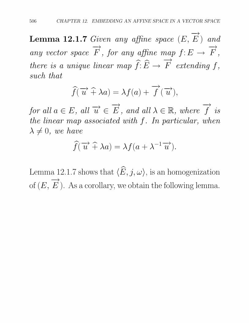
Lemma 12.1.7 Given any affine space (E,−→E ) and
any vector space−→F , for any affine map f : E → −→
F ,
there is a unique linear map f : E → −→F extending f ,
such that
f (−→u + λa) = λf (a) +−→f (−→u ),
for all a ∈ E, all −→u ∈ −→E , and all λ ∈ R, where
−→f is
the linear map associated with f . In particular, whenλ = 0, we have
f (−→u + λa) = λf (a + λ−1−→u ).
Lemma 12.1.7 shows that 〈E, j, ω〉, is an homogenization
of (E,−→E ). As a corollary, we obtain the following lemma.
12.1. THE “HAT CONSTRUCTION” 507
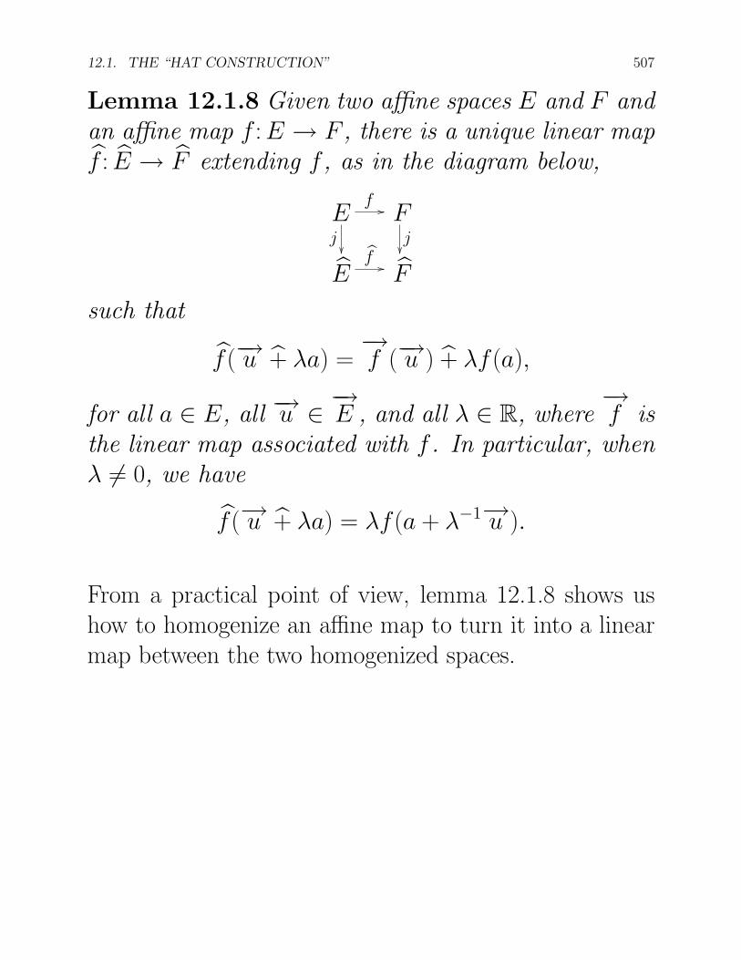
Lemma 12.1.8 Given two affine spaces E and F andan affine map f : E → F , there is a unique linear mapf : E → F extending f , as in the diagram below,
Ef
j
Fj
Ef
F
such that
f (−→u + λa) =−→f (−→u ) + λf (a),
for all a ∈ E, all −→u ∈ −→E , and all λ ∈ R, where
−→f is
the linear map associated with f . In particular, whenλ = 0, we have
f (−→u + λa) = λf (a + λ−1−→u ).
From a practical point of view, lemma 12.1.8 shows ushow to homogenize an affine map to turn it into a linearmap between the two homogenized spaces.
508 CHAPTER 12. EMBEDDING AN AFFINE SPACE IN A VECTOR SPACE
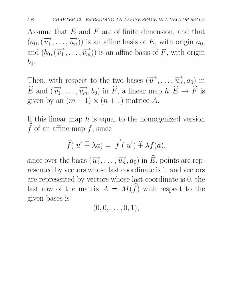
Assume that E and F are of finite dimension, and that
(a0, (−→u1 , . . . ,
−→un)) is an affine basis of E, with origin a0,
and (b0, (−→v1 , . . . ,−→vm)) is an affine basis of F , with origin
b0.
Then, with respect to the two bases (−→u1 , . . . ,−→un, a0) in
E and (−→v1 , . . . ,−→vm, b0) in F , a linear map h: E → F isgiven by an (m + 1) × (n + 1) matrice A.
If this linear map h is equal to the homogenized versionf of an affine map f , since
f (−→u + λa) =−→f (−→u ) + λf (a),
since over the basis (−→u1 , . . . ,−→un, a0) in E, points are rep-
resented by vectors whose last coordinate is 1, and vectorsare represented by vectors whose last coordinate is 0, thelast row of the matrix A = M(f ) with respect to thegiven bases is
(0, 0, . . . , 0, 1),
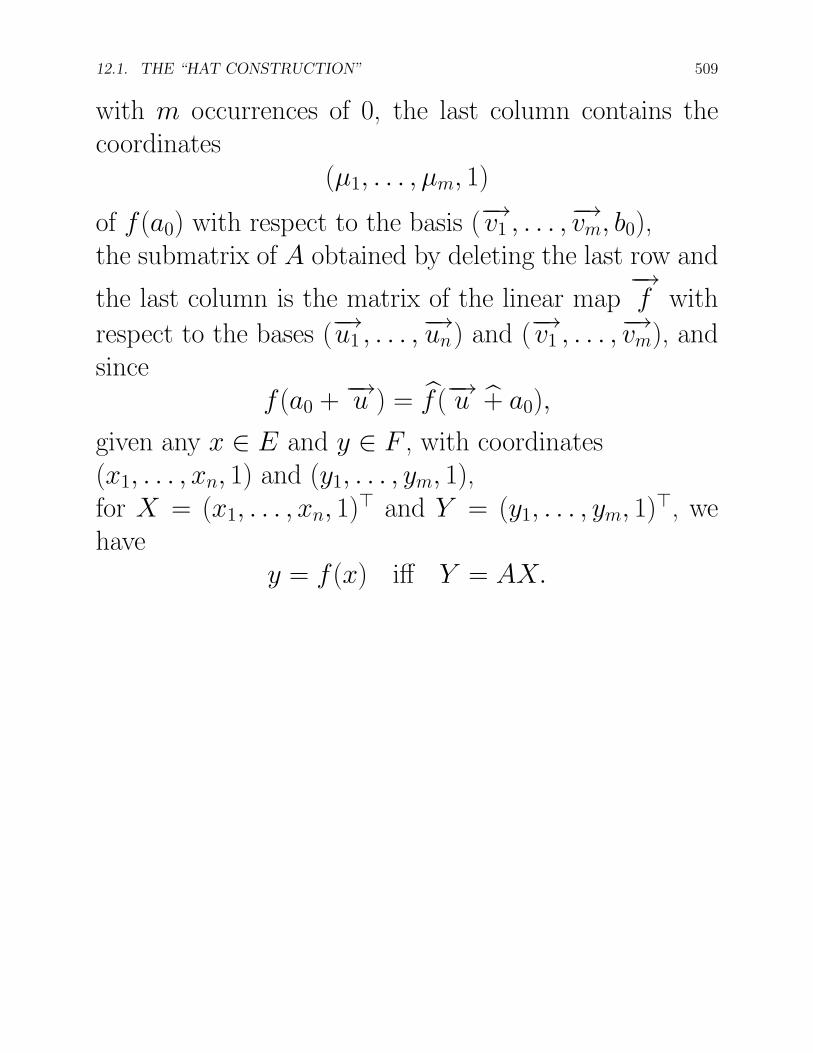
12.1. THE “HAT CONSTRUCTION” 509
with m occurrences of 0, the last column contains thecoordinates
(µ1, . . . , µm, 1)
of f (a0) with respect to the basis (−→v1 , . . . ,−→vm, b0),the submatrix of A obtained by deleting the last row and
the last column is the matrix of the linear map−→f with
respect to the bases (−→u1 , . . . ,−→un) and (−→v1 , . . . ,−→vm), and
sincef (a0 + −→u ) = f (−→u + a0),
given any x ∈ E and y ∈ F , with coordinates(x1, . . . , xn, 1) and (y1, . . . , ym, 1),for X = (x1, . . . , xn, 1) and Y = (y1, . . . , ym, 1), wehave
y = f (x) iff Y = AX.
510 CHAPTER 12. EMBEDDING AN AFFINE SPACE IN A VECTOR SPACE
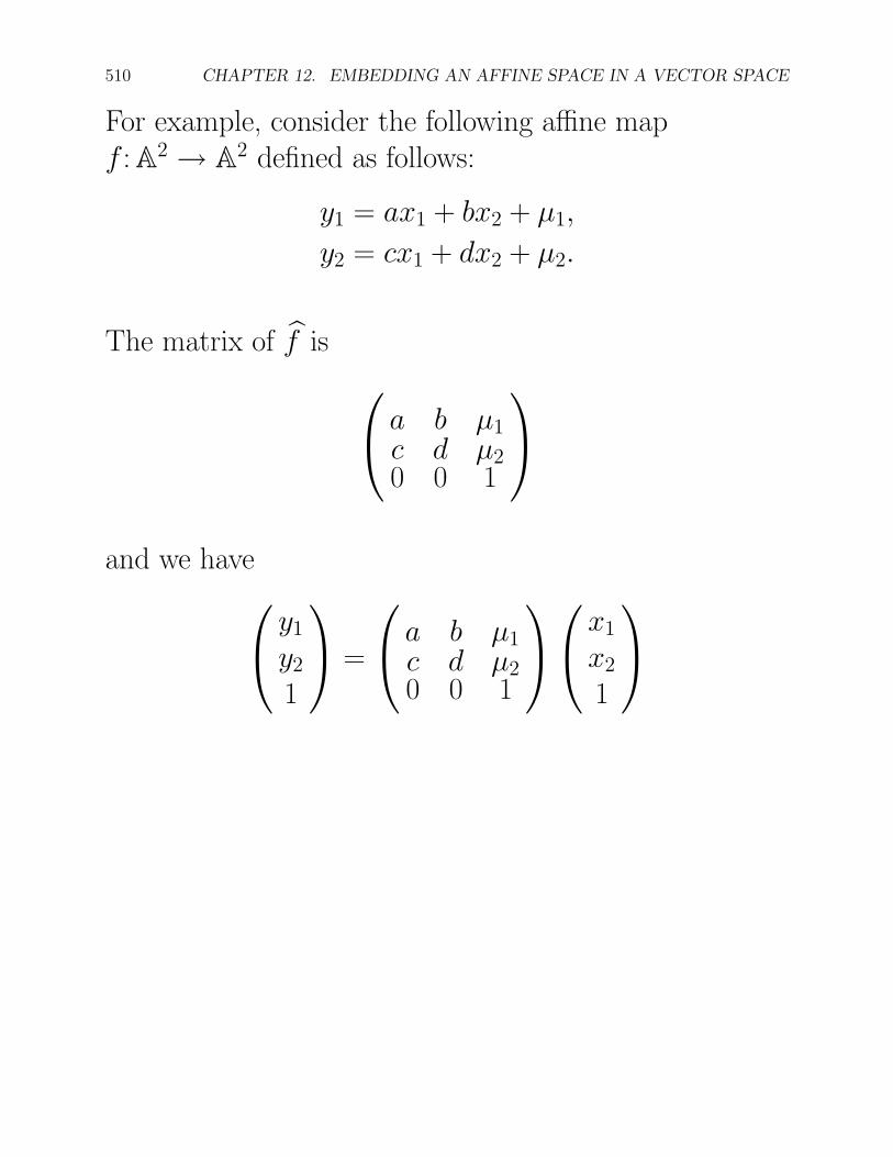
For example, consider the following affine mapf : A2 → A
2 defined as follows:
y1 = ax1 + bx2 + µ1,
y2 = cx1 + dx2 + µ2.
The matrix of f is a b µ1c d µ20 0 1
and we have y1
y2
1
=
a b µ1c d µ20 0 1
x1
x2
1
12.1. THE “HAT CONSTRUCTION” 511
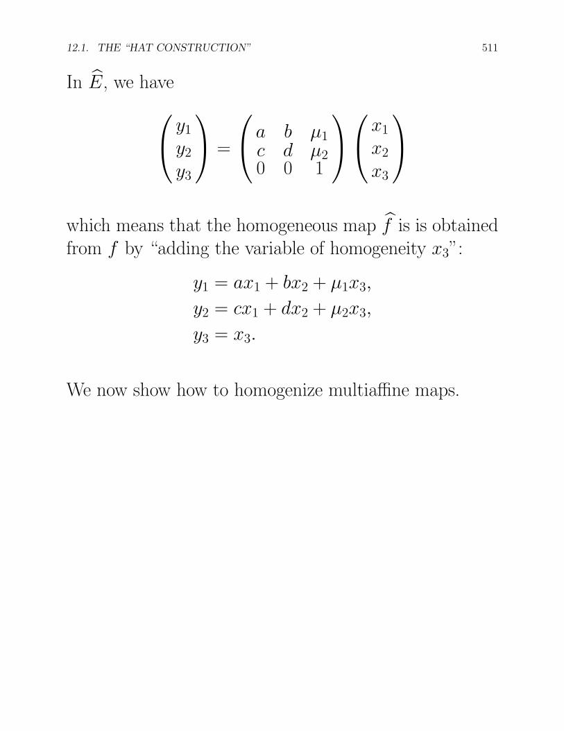
In E, we have y1
y2
y3
=
a b µ1c d µ20 0 1
x1
x2
x3
which means that the homogeneous map f is is obtainedfrom f by “adding the variable of homogeneity x3”:
y1 = ax1 + bx2 + µ1x3,
y2 = cx1 + dx2 + µ2x3,
y3 = x3.
We now show how to homogenize multiaffine maps.
512 CHAPTER 12. EMBEDDING AN AFFINE SPACE IN A VECTOR SPACE
Lemma 12.1.9 Given any affine space E and any
vector space−→F , for any m-affine map f : Em → −→
F ,
there is a unique m-linear map f : (E)m → −→F extend-
ing f , such that, if
f (a1 + −→v1 , . . . , am + −→vm) = f (a1, . . . , am) +∑S⊆1,...,m, k=card(S)
S=i1,...,ik, k≥1
fS(−→vi1 , . . . ,−→vik),
for all a1 . . . , am ∈ E, and all −→v1 , . . . ,−→vm ∈ −→E , where
the fS are uniquely determined multilinear maps (bylemma ??), then
f (−→v1 + λ1a1, . . . ,−→vm + λmam)
= λ1 · · ·λmf (a1, . . . , am) +∑S⊆1,...,m, k=card(S)
S=i1,...,ik, k≥1
(∏
j∈1,...,mj /∈S
λj) fS(−→vi1 , . . . ,−→vik),
for all a1 . . . , am ∈ E, all −→v1 , . . . ,−→vm ∈ −→E , and all
λ1, . . . , λm ∈ R. Furthermore, for λi = 0, 1 ≤ i ≤ m,we have
f (−→v1 + λ1a1, . . . ,−→vm + λmam) =
λ1 · · ·λmf (a1 + λ−11−→v1 , . . . , am + λ−1
m−→vm).
12.2. DIFFERENTIATING AFFINE POLYNOMIAL FUNCTIONS 513
12.2 Differentiating Affine Polynomial Functions Us-
ing Their Homogenized Polar Forms, Osculating
Flats
Let δ =−→1 , the unit (vector) in R. When dealing with
derivatives, it is also more convenient to denote the vector−→ab as b − a.
For any a ∈ A, the derivative DF (a) is the limit,
limt→0, t=0
F (a + tδ) − F (a)
t,
if it exists.
However, since F agrees with F on A, we have
F (a + tδ) − F (a) = F (a + tδ) − F (a),
and thus, we need to see what is the limit of
F (a + tδ) − F (a)
t,
when t → 0, t = 0, with t ∈ R.
514 CHAPTER 12. EMBEDDING AN AFFINE SPACE IN A VECTOR SPACE
Recall that since F : A → E , where E is an affine space,
the derivative DF (a) of F at a is a vector in−→E , and
not a point in E .
However, the structure of E takes care of this, sinceF (a + tδ) − F (a) is indeed a vector (remember our con-vention that − is an abbreviation for − ).
SinceF (a + tδ) = f (a + tδ, . . . , a + tδ︸ ︷︷ ︸
m
),
where f is the homogenized version of the polar form fof F , and F is the homogenized version of F , since
F (a + tδ)− F (a) = f (a + tδ, . . . , a + tδ︸ ︷︷ ︸m
)− f (a, . . . , a︸ ︷︷ ︸m
),
by multilinearity and symmetry, we have
F (a + tδ) − F (a) =
m t f (a, . . . , a︸ ︷︷ ︸m−1
, δ) +
k=m∑k=2
(mk
)tk f (a, . . . , a︸ ︷︷ ︸
m−k
, δ, . . . , δ︸ ︷︷ ︸k
),
and thus,
limt→0, t=0
F (a + tδ) − F (a)
t= mf (a, . . . , a︸ ︷︷ ︸
m−1
, δ).
12.2. DIFFERENTIATING AFFINE POLYNOMIAL FUNCTIONS 515
However, since F extends F on A, we haveDF (a) = DF (a), and thus, we showed that
DF (a) = mf (a, . . . , a︸ ︷︷ ︸m−1
, δ).
This shows that the derivative of F at a ∈ A can becomputed by evaluating the homogenized version f ofthe polar form f of F , by replacing just one occurrenceof a in f (a, . . . , a) by δ.
516 CHAPTER 12. EMBEDDING AN AFFINE SPACE IN A VECTOR SPACE
More generally, we have the following useful lemma.
Lemma 12.2.1 Given an affine polynomial functionF : A → E of polar degree m, where E is a normedaffine space, the k-th derivative DkF (a) can be com-
puted from the homogenized polar form f of F as fol-lows, where 1 ≤ k ≤ m:
DkF (a) = m(m−1) · · · (m−k+1) f (a, . . . , a︸ ︷︷ ︸m−k
, δ, . . . , δ︸ ︷︷ ︸k
).
Since coefficients of the form m(m − 1) · · · (m − k + 1)occur a lot when taking derivatives, following Knuth, it isuseful to introduce the falling power notation. We definethe falling power mk, as
mk = m(m − 1) · · · (m − k + 1),
for 0 ≤ k ≤ m, with m0 = 1, and with the conventionthat mk = 0 when k > m.
Using the falling power notation, the previous lemmareads as
DkF (a) = mk f (a, . . . , a︸ ︷︷ ︸m−k
, δ, . . . , δ︸ ︷︷ ︸k
).
12.2. DIFFERENTIATING AFFINE POLYNOMIAL FUNCTIONS 517
We also get the following explicit formula in terms ofcontrol points.
Lemma 12.2.2 Given an affine polynomial functionF : A → E of polar degree m, where E is a normedaffine space, for any r, s ∈ A, with r = s, the k-th derivative DkF (r) can be computed from the polarform f of F as follows, where 1 ≤ k ≤ m:
DkF (r) =mk
(s − r)k
i=k∑i=0
(ki
)(−1)k−i f (r, . . . , r︸ ︷︷ ︸
m−i
, s, . . . , s︸ ︷︷ ︸i
).
If F is specified by the sequence of m + 1 control pointsbi = f (r m−i s i), 0 ≤ i ≤ m, the above lemma showsthat the k-th derivative DkF (r) of F at r, depends onlyon the k + 1 control points b0, . . . , bk
In terms of the control points b0, . . . , bk, the formula oflemma ?? reads as follows:
DkF (r) =mk
(s − r)k
i=k∑i=0
(ki
)(−1)k−i bi.
518 CHAPTER 12. EMBEDDING AN AFFINE SPACE IN A VECTOR SPACE
In particular, if b0 = b1, then DF (r) is the velocity vectorof F at b0, and it is given by
DF (r) =m
s − r
−−→b0b1 =
m
s − r(b1 − b0),
the last expression making sense in E .
In terms of the de Casteljau diagram
DF (t) =m
s − r(b1,m−1 − b0,m−1).
Similarly, the acceleration vector D2F (r) is given by
D2F (r) =m(m − 1)
(s − r)2(−−→b0b2 − 2
−−→b0b1) =
m(m − 1)
(s − r)2(b2 − 2b1 + b0),
the last expression making sense in E .
Later on when we deal with surfaces, it will be necessaryto generalize the above results to directional derivatives.However, we have basically done all the work already.
12.2. DIFFERENTIATING AFFINE POLYNOMIAL FUNCTIONS 519
Let us assume that E and E are normed affine spaces,and consider a map F : E → E .
Recall from definition ??, that if A is any open subset of
E, for any a ∈ A, for any −→u = −→0 in
−→E , the directional
derivative of F at a w.r.t. the vector −→u , denoted asDuF (a), is the limit, if it exists,
limt→0,t∈U,t=0
F (a + t−→u ) − F (a)
t,
where U = t ∈ R | a + t−→u ∈ A.
If F : E → E is a polynomial function of degree m, withpolar form the symmetric multiaffine map f : Em → E ,then
F (a + t−→u ) − F (a) = F (a + t−→u ) − F (a),
where F is the homogenized version of F , that is, thepolynomial map F : E → E associated with the homoge-nized version f : (E)m → E of the polar form f : Em → Eof F : E → E .
520 CHAPTER 12. EMBEDDING AN AFFINE SPACE IN A VECTOR SPACE
Thus, DuF (a) exists iff the limit
limt→0, t=0
F (a + t−→u ) − F (a)
t
exists, and in this case, this limit is DuF (a) = DuF (a).We get
DuF (a) = mf (a, . . . , a︸ ︷︷ ︸m−1
,−→u ).
By a simple, induction, we can prove the following lemma.
Lemma 12.2.3 Given an affine polynomial functionF : E → E of polar degree m, where E and E are
normed affine spaces, for any k nonzero vectors −→u1 ,
. . ., −→uk ∈ −→E , where 1 ≤ k ≤ m, the k-th directional
derivative Du1 . . . DukF (a) can be computed from the
homogenized polar form f of F as follows:
Du1 . . . DukF (a) = mk f (a, . . . , a︸ ︷︷ ︸
m−k
,−→u1 , . . . ,−→uk ).
If E has finite dimension,
DkF (a)(−→u1 , . . . ,−→uk ) = mk f (a, . . . , a︸ ︷︷ ︸
m−k
,−→u1 , . . . ,−→uk ).