Chapter 12 Consumption, Real GDP, and the Multiplier

Chapter 12

Consumption, Real GDP,and the Multiplier

Slide 12-2

Introduction

Investment spending by businesses is a key component of economic growth.

Expenditures on information technology were once expected to provide a bigger push to GDP expansion than they have. Why might investment spending and its effect on GDP be rather unpredictable?

Slide 12-3

Learning Objectives

Distinguish between saving and savings and explain how consumption and saving are related

Explain the key determinants of consumption and saving in the Keynesian model

Identify the primary determinants of planned investment

Slide 12-4

Learning Objectives

Describe how equilibrium national income is established in the Keynesian model

Evaluate why autonomous changes in total planned expenditures have a multiplier effect on equilibrium national income

Understand the relationship between total planned expenditures and the aggregate demand curve

Slide 12-5

Chapter Outline

Some Simplifying Assumptions in the Keynesian Model

Determinants of Planned Consumption and Planned Saving

Determinants of Investment

Consumption as a Function of Real GDP

Slide 12-6

Chapter Outline

Saving and Investment: Planned versus Actual

Keynesian Equilibrium with Government and the Foreign Sector Added

The Multiplier

Slide 12-7

Chapter Outline

The Multiplier Effect When the Price Level Can Change

The Multiplier Effect on the Equilibrium Level of Real GDP

Slide 12-8

Did You Know That...

Historically, investment spending has been the most volatile component of GDP?

Economist John Maynard Keynes put forth one of the first theories about the relationship among personal consumption, investment spending, and economic growth?

Slide 12-9

Keynes revisited

– Aggregate demand determines output (horizontal SRAS)

– We will examine the elements of aggregate demand (AD = C + I + G + X)

– Prices are fixed, so output is in real terms

Some Simplifying Assumptions in a Keynesian Model

Slide 12-10

Assumptions

– Businesses pay no indirect taxes (sales tax)

– Businesses distribute all profits to shareholders

– There is no depreciation

– The economy is closed


Slide 12-11

Definitions and relationships revisited– Consumption

• Spending on new goods and services out of a household’s current income

– Saving• The act of not consuming all of one’s income

– Savings• Accumulation of past saving; a stock variable


Slide 12-12


Disposable income equals consumption plus saving.

This accounting identity shows that each dollar of take-home income can either be spent or saved.

Slide 12-13

Investment– The spending by business on things

which can be used to produce goods and services in the future


Slide 12-14

Keynes was concerned with changes in AD.


AD = C + I + G + X

Slide 12-15

Keynes argued that saving and consumption decisions depend primarily on an individual’s real disposable income.

Consumption Function– The relationship between planned

consumption expenditures and their current level of real income


Slide 12-16

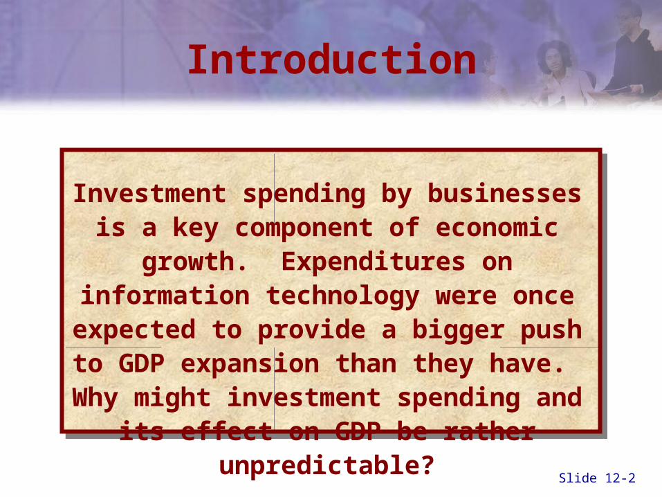
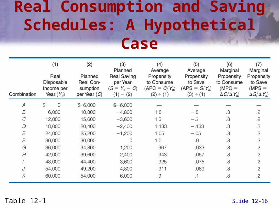
Real Consumption and Saving Schedules: A Hypothetical Case

Table 12-1

Slide 12-17

C = Yd

45o

Consumption function

The Consumption and Saving Functions

Real Disposable Income (Yd dollars per year)

Pla

nned

Rea

l Con

sum

ptio

n(C

, do

llars

per

yea

r)

12,000 24,000 36,0000

6,000

12,000

24,000

36,000

48,000

48,000 60,000

60,000

Break-even income

AB

C

DE

FG

H

I

J

K

Figure 12-1

Slide 12-18

The Consumption and Saving Functions


Pla

nned

Rea

l Con

sum

ptio

n(C

, do

llars

per

yea

r)

12,000 24,000 36,0000

6,000

12,000

24,000

36,000

48,000

48,000 60,000

C = Yd60,000

Break-even income

Consumption function

AB

C

DE

FG

H

I

J

K

45o

Dissaving

Saving

Autonomousconsumption

(Equ

al v

ert

ical

dis

tanc

e)

Figure 12-1

Slide 12-19

The Consumptionand Saving Functions

0

6,000

-6,000

12,000

36,000 48,000 60,000

24,000


Pla

nned

Rea

l Sav

ing

(S,

dolla

rs p

er y

ear)

CB

A

DE

F

GH

IJ

K

Figure 12-1

Slide 12-20

The Consumptionand Saving Functions

0

6,000

-6,000

12,000

36,000 48,000 60,000

24,000


Pla

nned

Rea

l Sav

ing

(S,

dolla

rs p

er y

ear)

CB

A

DE

F

GH

IJ

K

Saving

Dissaving

Figure 12-1

Slide 12-21

Dissaving

– Negative saving; spending exceeds income

Autonomous Consumption

– The part of consumption that is independent of the level of disposable income


Slide 12-22

Average Propensity to Consume (APC)

– Consumption divided by disposable income

– The proportion of total disposable income that is consumed


APC =real consumption

real disposable income

Slide 12-23

Average Propensity to Save (APS)

– Saving divided by disposable income

– The proportion of total disposable income that is saved


APS =real saving

real disposable income

Slide 12-24

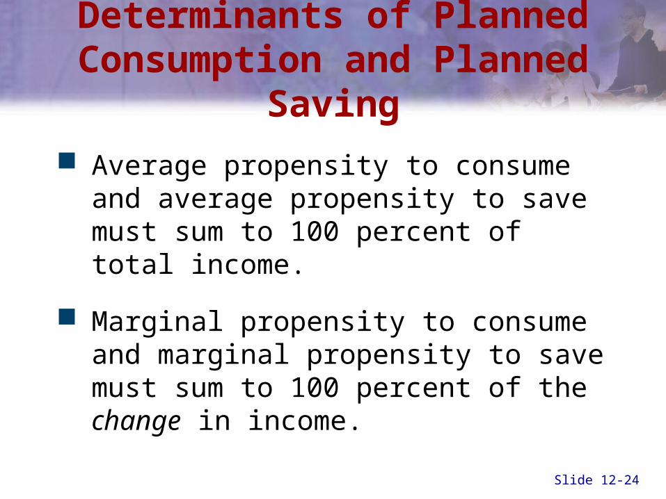
Average propensity to consume and average propensity to save must sum to 100 percent of total income.

Marginal propensity to consume and marginal propensity to save must sum to 100 percent of the change in income.


Slide 12-25

Example– Income = $54,000

– C = $49,200

– S = $4,800

What is the APC?


APC =$49,200

$54,000= .911

Slide 12-26

Example– Income increases by $6,000 to $60,000

– C = $54,000

– S = $6,000

What is the APC?


APC =$54,000

$60,000= .90

Slide 12-27

Marginal Propensity to Consume (MPC)

– The ratio of the change in consumption to the change in disposable income


MPC =change in consumption

change in real disposable income

Slide 12-28

Marginal Propensity to Save (MPS)

– The ratio of the change in saving to the change in disposable income


MPS =change in saving

change in real disposable income

Slide 12-29

Causes of shifts in the consumption function– Non-income determinants of consumption

• Population• Wealth

Can you think of other non-income determinants of consumption?


Slide 12-30

International Example:Determinants of Investment Spending

Investment expenditures by Japanese businesses were depressed throughout the 1990’s, even though interest rates were close to zero.

The low cost of borrowing was not enough to offset the effect of poor prospects for growth in consumer spending.

Slide 12-31

International Example:Determinants of Investment Spending

Investment spending in Japan recovered only in 2002, as firms began to anticipate higher sales.

Firms began replacing old equipment, and in some cases actually expanded their productive capacity.

Slide 12-32

Consumption as a Function of Real GDP

Figure 12-3

Slide 12-33

Determinants of Investment

Historically

– Investment has been more volatile than consumption

Why?

AD = C + I + G + X

Slide 12-34

Combining Consumptionand Investment

Figure 12-4, Panel (c)

Slide 12-35

Saving and Investment:Planned versus Actual

Equilibrium

– The intersection of the planned saving and planned investment schedules

No tendency for businesses to alter the rate of production or the level of employment

– There are no unplanned inventory changes

Slide 12-36

Planned and Actual Ratesof Saving and Investment

Real GDP per Year($ trillions)

7.0 8.0 9.00

1.2

1.6

2.0

2.4

10.0 11.0

I

Sav

ing

and

Inve

stm

ent

per

Yea

r ($

tril

lions

) S

Actual S = actual I

Unplanned inventory decrease = $400 billion per year

E

Figure 12-5

Slide 12-37

Planned and Actual Ratesof Saving and Investment


7.0 8.0 9.00

1.2

1.6

2.0

2.4

10.0 11.0

E

S

I

Sav

ing

and

Inve

stm

ent

per

Yea

r ($

tril

lions

)

Actual S = actual I

Unplanned inventory decrease = $400 billion per year

Unplanned inventory increase = $400 billion per year

Planned investment = $1.600 trillion per year

Figure 12-5

Actual S = actual I

Slide 12-38

Government (G)—C + I + G– Federal, state, and local

• Does not include transfer payments• Is autonomous• Lump-sum taxes = G

Lump-Sum Tax– A tax that does not depend on income or

the circumstances of the taxpayer

Keynesian Equilibrium withGovernment and the Foreign Sector

Slide 12-39

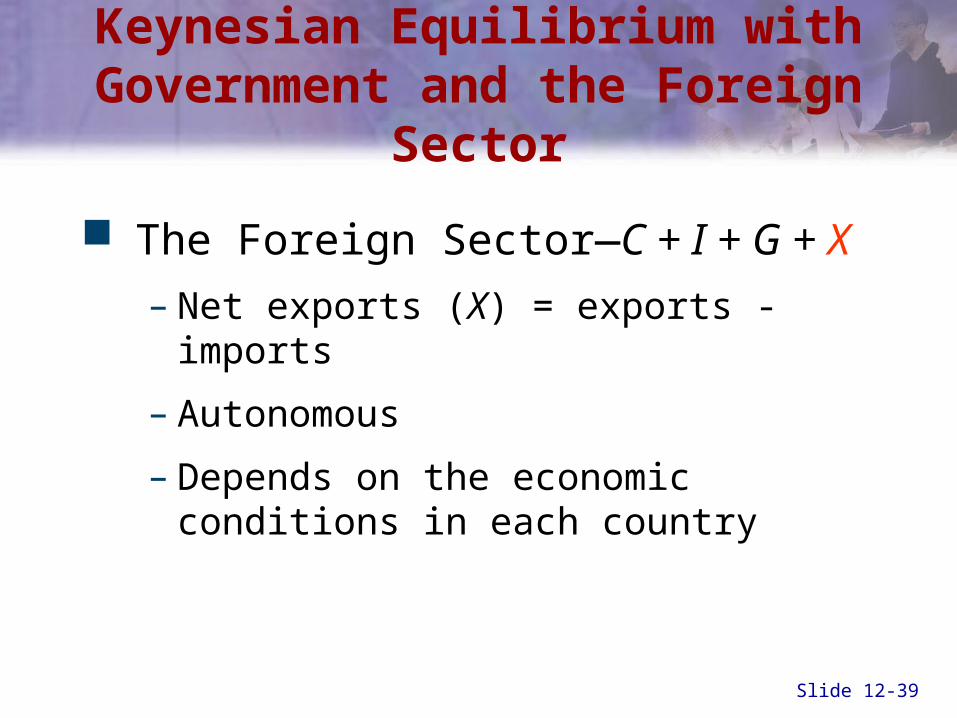
The Foreign Sector—C + I + G + X

– Net exports (X) = exports - imports

– Autonomous

– Depends on the economic conditions in each country

Keynesian Equilibrium withGovernment and the Foreign Sector

Slide 12-40

The Determination of EquilibriumReal GDP with Net Exports

Table 12-2

Slide 12-41

The Equilibrium Levelof Real GDP

Figure 12-6

Slide 12-42

The Equilibrium Levelof Real GDP

Observations– If C + I + G + X = Y

• Equilibrium

– If C + I + G + X > Y • Unplanned drop in inventories• Businesses increase output• Y returns to equilibrium

– If C + I + G + X < Y• Unplanned rise in inventories• Businesses cut output• Y returns to equilibrium

Slide 12-43

The Multiplier

Multiplier

– The ratio of the change in the equilibrium level of real national income to the change in autonomous expenditures

Slide 12-44

The Multiplier

Question

– How can $1.1 trillion of I generate $5.5 trillion of Y?

Answer

– The autonomous spending multiplier

Slide 12-45

The Multiplier ProcessAssumption: MPC = .8 or 4/5

Annual Increase Annual Increase Annual Increasein Real in Planned in Planned

National Income Consumption SavingRound ($ billions) ($ billions) ($ billions)

1 ($100 billion per year increase in I) 100.00 80.000 20.000

2 80.00 64.00 16.000

3 64.00 51.200 12.800

4 51.20 40.960 10.240

5 40.96 32.768 8.192

. . . .

. . . .

. . . .

All later rounds 163.84 131.072 32.768

Totals (C+I+G) 500.00 400.00 100.000

Table 12-3

Slide 12-46

The Multiplier

The multiplier formula

Multiplier = 11 - MPC

= 1MPS

Slide 12-47

The Multiplier

Examples

MPC =34

MPS =14

Mult. =1

1/4= 4

MPC =45

MPS =15

Mult. =1

1/5= 5

MPC =23

MPS =13

Mult. =1

1/3= 3

MPC =79

MPS =29

Mult. =1

9/2= 4.5

MPC =35

MPS =25

Mult. =1

5/2= 2.5

Slide 12-48

The Multiplier

Question

– How does the size of the MPC influence the value of the multiplier?

Answer

– The smaller the MPS, the larger the multiplier

– The larger the MPC, the larger the multiplier

Slide 12-49

The Multiplier

Measuring the change in equilibrium income from a change in autonomous spending

Change in equilibrium income = multiplier x change in level of real autonomous spending

Slide 12-50

The Multiplier

Question

– What does the multiplier tell us about the potential impact on the economy for a change in autonomous spending?

Slide 12-51

Example: A Double-Whammy Multiplier Effect

At the end of 2003, both investment spending and net exports increased for the U.S. economy.

This amounted to a significant increase in autonomous spending.

Due to the multiplier effect, the rate of overall GDP growth exceeded predictions.

Slide 12-52

The Multiplier Effect Whenthe Price Level Can Change

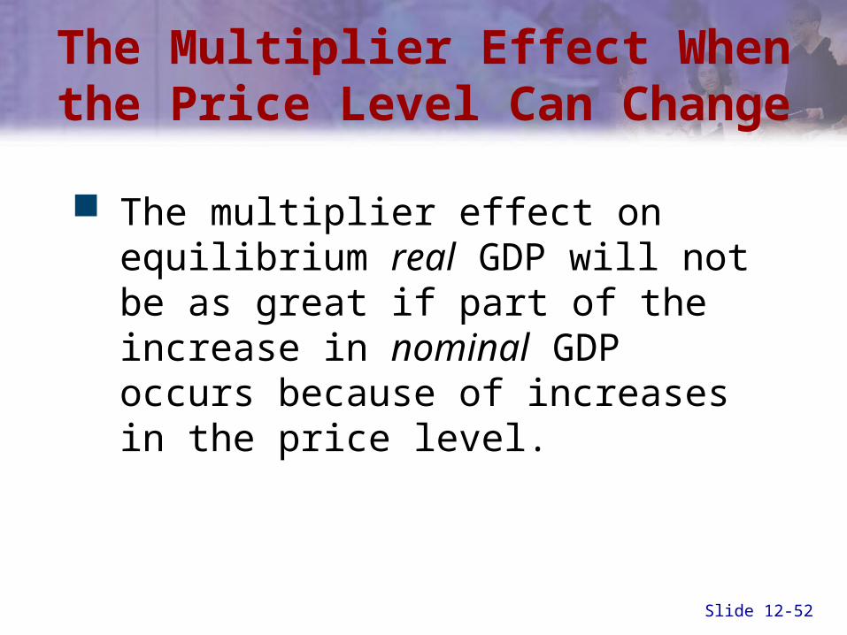
The multiplier effect on equilibrium real GDP will not be as great if part of the increase in nominal GDP occurs because of increases in the price level.

Slide 12-53

The Multiplier Effect onthe Equilibrium Level of Real GDP

0

Pric

e Le

vel

AD1

12.0

LRAS SRAS

120

AD2

With $100 billion increase in autonomous spending

Real GDP per Year($ trillions)Figure 12-7

Slide 12-54



12.00

Pric

e Le

vel

AD2

SRASLRAS

AD1

• With price adjustment the multiplier effect is less

• Real national income increases to $12.3 billion

With $100 billion increase in autonomous spending

125

12.3

120

12.5

Figure 12-7

Slide 12-55



Con

sum

ptio

n, I

nves

tmen

t,

Gov

ernm

ent

Pur

chas

es,

and

Net

Exp

orts

(C + I + G + X)100

E1

12

Figure 12-8

Slide 12-56



Con

sum

ptio

n, I

nves

tmen

t,

Gov

ernm

ent

Pur

chas

es,

and

Net

Exp

orts

(C + I + G + X)100

E1

(C + I + G + X)125

E2

10 12

Figure 12-8

Slide 12-57



Con

sum

ptio

n, I

nves

tmen

t,

Gov

ernm

ent

Pur

chas

es,

and

Net

Exp

orts

(C + I + G + X)100

12

E1

(C + I + G + X)125

• Assume prices increase to 125• C + I + G + X decreases• Equilibrium Y falls to $10 trillion

10

E2

Figure 12-8

Slide 12-58

Issues and Applications: “New Economy” or New Source of

Volatility?

Proponents of a theory of the “new economy” argued in the 1990’s that information technology expenditures would eliminate any economic downturns

– By making firms more productive

– By buoying investment spending

While IT expenditures contribute to growth of real GDP, they remain a source of volatility.

Slide 12-59

Summary Discussion of Learning Objectives

The difference between saving and savings and the relationship between consumption and saving is a flow over time while savings is a stock consumption plus saving equals disposable income.

The key determinant of consumption and saving in the Keynesian model is disposable income.

Slide 12-60


The primary determinants of planned investment are the interest rate, business expectations, productive technology, and business taxes.

Slide 12-61


In the Keynesian model equilibrium national income occurs where the C + I + G + X schedule crosses the 45 degree line.

Autonomous changes in total planned expenditure have a multiplier effect on equilibrium national income because an increase in autonomous expenditures increases income which increases consumption.

Slide 12-62


The relationship between total planned expenditures and the aggregate demand curve is inverse. An increase in the price level reduces planned expenditures.

– Real balance effect

– Interest rate effect

– Open economy effect

End of Chapter 12Consumption, Real GDP,and the Multiplier

Documents

Chapter 12 Consumption, Real GDP, and the Multiplier