Chapter 12: Band Combinations using Landsat Imagery …virginiaview.cnre.vt.edu/tutorial/Chapter_12_Band... · · 2014-10-03Using different band combinations to display your scene

Chapter 12: Band Combinations using Landsat Imagery

Remote Sensing Analysis

in an

ArcMap Environment

Tammy E. Parece

Remote Sensing in an ArcMap Environment

Tammy Parece James Campbell

John McGee

This workbook is available online as text (.pdf’s) and short video tutorials via: http://www.virginiaview.net/education.html

Image source: landsat.usgs.gov

NSF DUE 0903270; 1205110

http://www.virginiaview.net/education.html

The project described in this publication was supported by Grant Number G14AP00002 from the Department of the Interior, United States Geological Survey to AmericaView. Its contents are solely the responsibility of the authors; the views and conclusions contained in this document are those of the authors and should not be interpreted as representing the opinions or policies of the U.S. Government. Mention of trade names or commercial products does not constitute their endorsement by the U.S. Government.

Remote Sensing in an ArcMap Environment 12. Band Combinations Using Landsat Imagery

The instructional materials contained within these documents are copyrighted property of

VirginiaView, its partners and other participating AmericaView consortium members. These materials may be reproduced and used by educators for instructional purposes. No

permission is granted to use the materials for paid consulting or instruction where a fee is collected. Reproduction or translation of any part of this document beyond that permitted in

Section 107 or 108 of the 1976 United States Copyright Act without the permission of the copyright owner(s) is unlawful.

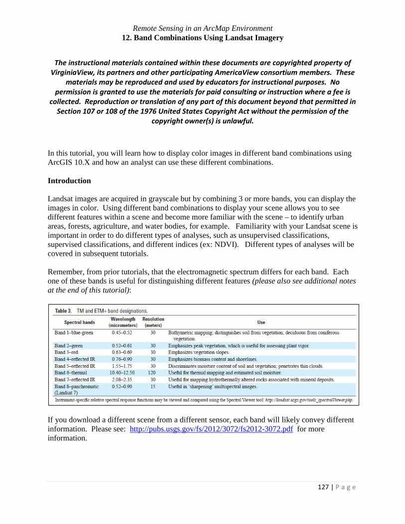
In this tutorial, you will learn how to display color images in different band combinations using ArcGIS 10.X and how an analyst can use these different combinations. Introduction Landsat images are acquired in grayscale but by combining 3 or more bands, you can display the images in color. Using different band combinations to display your scene allows you to see different features within a scene and become more familiar with the scene – to identify urban areas, forests, agriculture, and water bodies, for example. Familiarity with your Landsat scene is important in order to do different types of analyses, such as unsupervised classifications, supervised classifications, and different indices (ex: NDVI). Different types of analyses will be covered in subsequent tutorials. Remember, from prior tutorials, that the electromagnetic spectrum differs for each band. Each one of these bands is useful for distinguishing different features (please also see additional notes at the end of this tutorial):

If you download a different scene from a different sensor, each band will likely convey different information. Please see: http://pubs.usgs.gov/fs/2012/3072/fs2012-3072.pdf for more information.

127 | P a g e

http://pubs.usgs.gov/fs/2012/3072/fs2012-3072.pdf


Creating Different Band Combinations

Open ArcMap, open a new map document, and add the composite image that was created

in the tutorial on Creating a Composite Image from Landsat Imagery. Set your Workspace. You

will not need the Image Analysis Window to display different band combinations.

Right click on your composite image in the Table of Contents, go to Properties and click

on the Symbology tab. This tab looks very different than it did when we were looking at the

image of a single band. The RGB Composite is highlighted (red oval) and multiple Channels

and Bands are listed (green oval).

Under Stretch, it lists the method that ArcMap used to stretch the colors over the range of

brightness values (remember each band has a range of brightness values). (Note – specific

discussion of the different methods is beyond this tutorial – please see ArcGIS Help or other

related sources for further information.)

128 | P a g e


Click on the Histograms button. ArcMap displays the histograms for each band

displayed in the red, green, or blue channels. These are frequency histograms which plot the

values of the digital numbers (DNs) (x-axis) against the number of pixels with that value (y-

axis). It shows the minimum DN value, and the maximum, mean, and standard deviation. Why

would each histogram look different?

(Answer – because each band has a different range of DNs.) We will discuss Histograms more in

the tutorial on Radiometric Enhancement of Landsat Imagery.

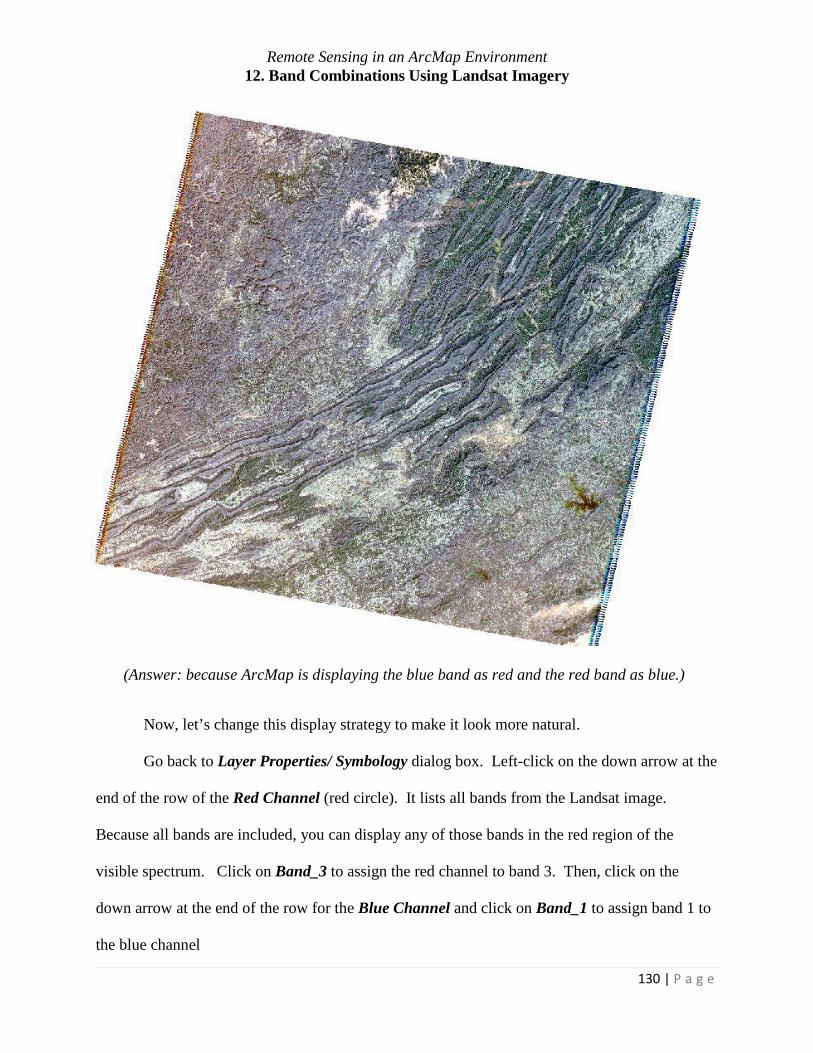
Close the dialog box and let’s next look at the image in the map document. The image

that is displayed in the map document window does not look very natural. Why?

129 | P a g e


(Answer: because ArcMap is displaying the blue band as red and the red band as blue.)

Now, let’s change this display strategy to make it look more natural.

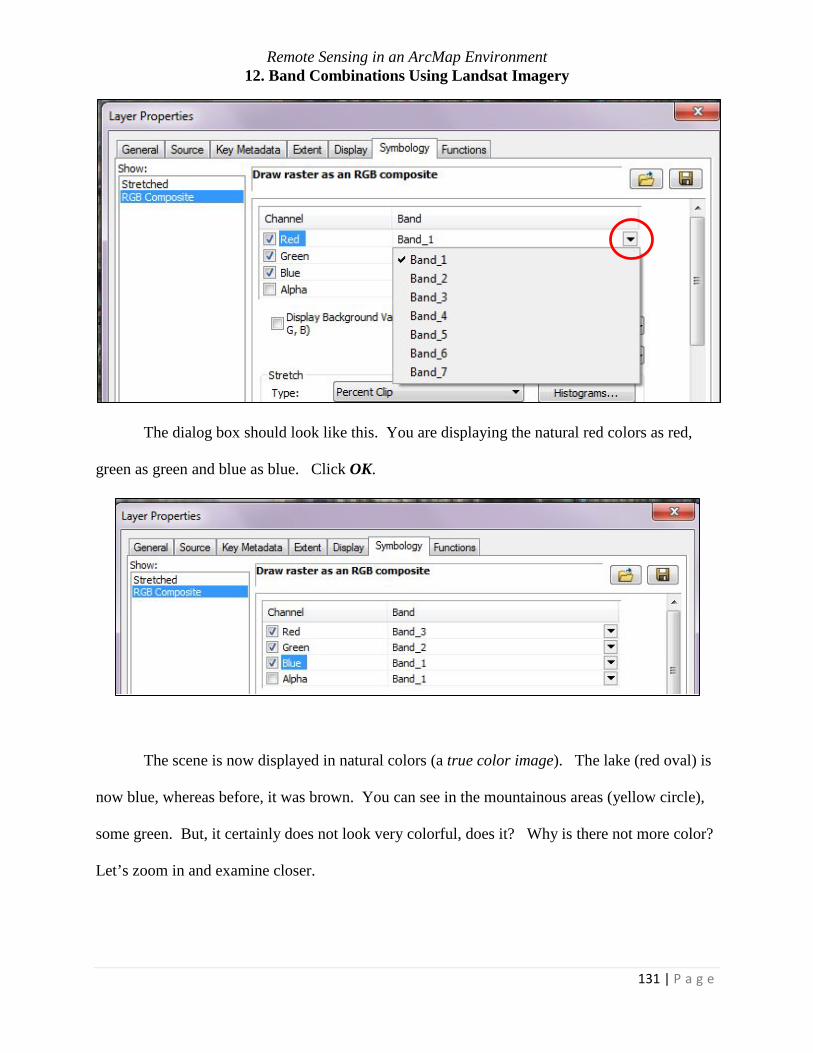
Go back to Layer Properties/ Symbology dialog box. Left-click on the down arrow at the

end of the row of the Red Channel (red circle). It lists all bands from the Landsat image.

Because all bands are included, you can display any of those bands in the red region of the

visible spectrum. Click on Band_3 to assign the red channel to band 3. Then, click on the

down arrow at the end of the row for the Blue Channel and click on Band_1 to assign band 1 to

the blue channel

130 | P a g e


The dialog box should look like this. You are displaying the natural red colors as red,

green as green and blue as blue. Click OK.

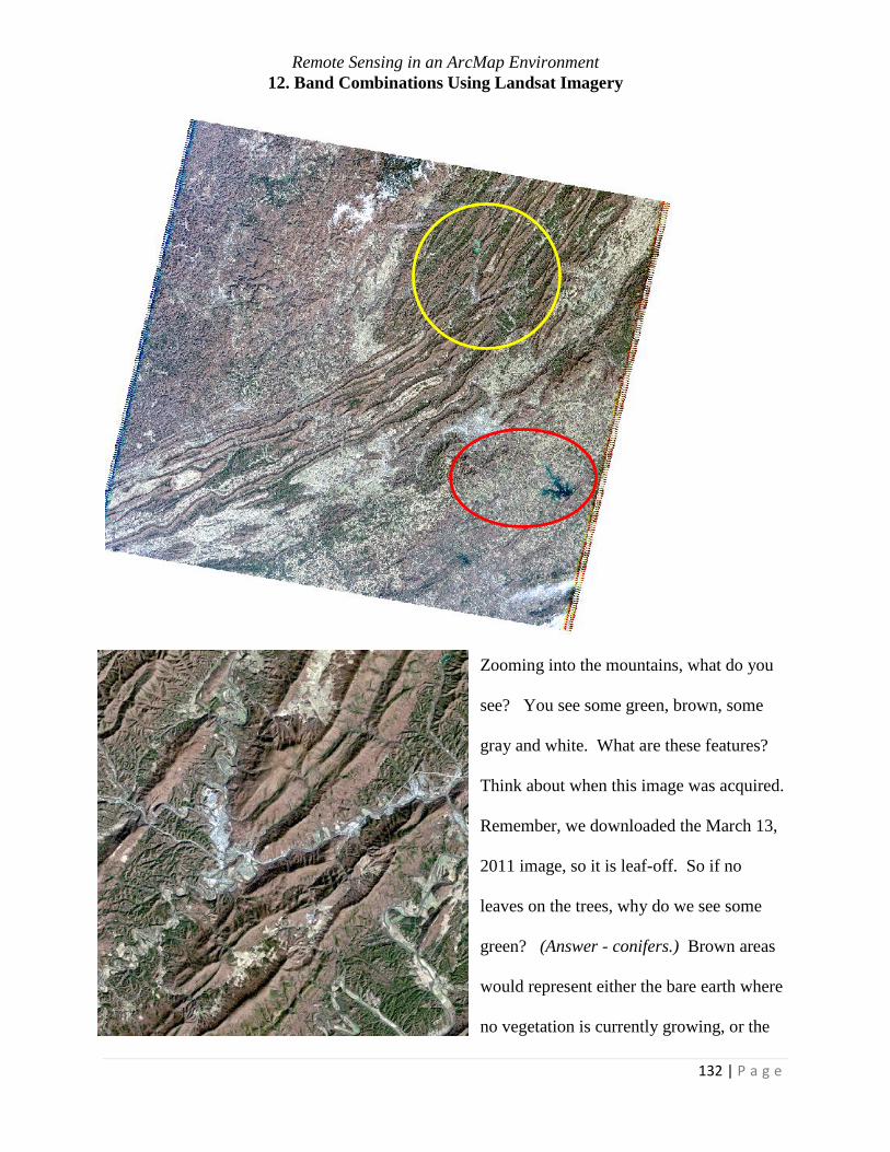
The scene is now displayed in natural colors (a true color image). The lake (red oval) is

now blue, whereas before, it was brown. You can see in the mountainous areas (yellow circle),

some green. But, it certainly does not look very colorful, does it? Why is there not more color?

Let’s zoom in and examine closer.

131 | P a g e


Zooming into the mountains, what do you

see? You see some green, brown, some

gray and white. What are these features?

Think about when this image was acquired.

Remember, we downloaded the March 13,

2011 image, so it is leaf-off. So if no

leaves on the trees, why do we see some

green? (Answer - conifers.) Brown areas

would represent either the bare earth where

no vegetation is currently growing, or the

132 | P a g e


deciduous trees. What about the white? What are long, linear features on the ground and could

possibly be seen from an overhead image?

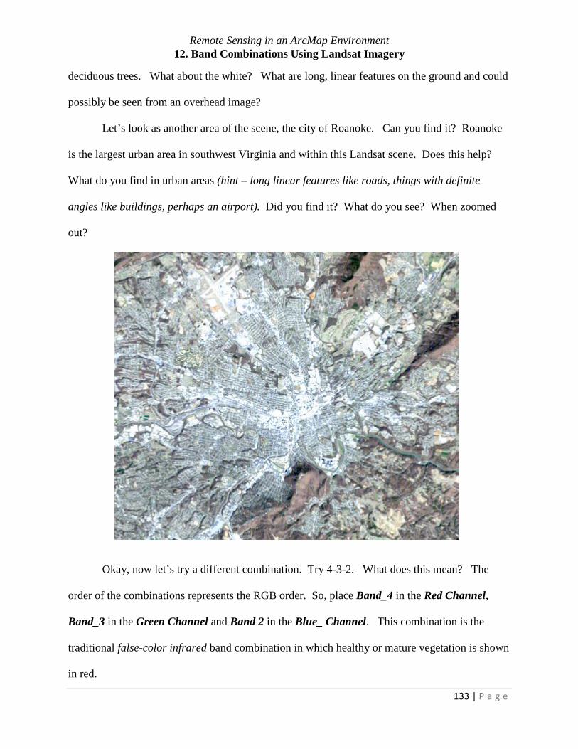
Let’s look as another area of the scene, the city of Roanoke. Can you find it? Roanoke

is the largest urban area in southwest Virginia and within this Landsat scene. Does this help?

What do you find in urban areas (hint – long linear features like roads, things with definite

angles like buildings, perhaps an airport). Did you find it? What do you see? When zoomed

out?

Okay, now let’s try a different combination. Try 4-3-2. What does this mean? The

order of the combinations represents the RGB order. So, place Band_4 in the Red Channel,

Band_3 in the Green Channel and Band 2 in the Blue_ Channel. This combination is the

traditional false-color infrared band combination in which healthy or mature vegetation is shown

in red.

133 | P a g e


Your dialog box should appear as follows:

Don’t forget to click OK before you close the window!

We were still zoomed into Roanoke. Looks a lot different doesn’t it? Why? What do

the different bands being placed within those specific channels mean? (See Landsat Table

above and additional notes at the end of this tutorial.) Landsat Band_4 is the near infrared and

134 | P a g e


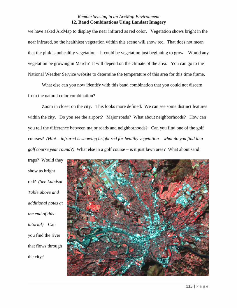
we have asked ArcMap to display the near infrared as red color. Vegetation shows bright in the

near infrared, so the healthiest vegetation within this scene will show red. That does not mean

that the pink is unhealthy vegetation – it could be vegetation just beginning to grow. Would any

vegetation be growing in March? It will depend on the climate of the area. You can go to the

National Weather Service website to determine the temperature of this area for this time frame.

What else can you now identify with this band combination that you could not discern

from the natural color combination?

Zoom in closer on the city. This looks more defined. We can see some distinct features

within the city. Do you see the airport? Major roads? What about neighborhoods? How can

you tell the difference between major roads and neighborhoods? Can you find one of the golf

courses? (Hint – infrared is showing bright red for healthy vegetation – what do you find in a

golf course year round?) What else in a golf course – is it just lawn area? What about sand

traps? Would they

show as bright

red? (See Landsat

Table above and

additional notes at

the end of this

tutorial). Can

you find the river

that flows through

the city?

135 | P a g e


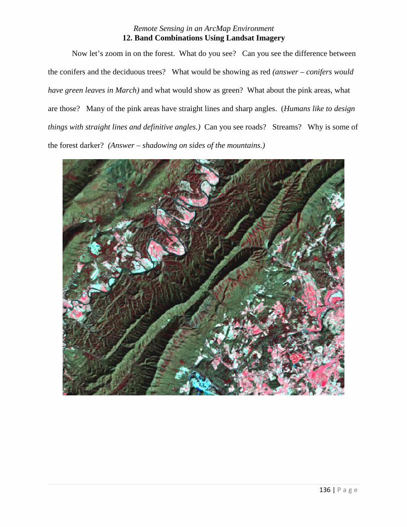
Now let’s zoom in on the forest. What do you see? Can you see the difference between

the conifers and the deciduous trees? What would be showing as red (answer – conifers would

have green leaves in March) and what would show as green? What about the pink areas, what

are those? Many of the pink areas have straight lines and sharp angles. (Humans like to design

things with straight lines and definitive angles.) Can you see roads? Streams? Why is some of

the forest darker? (Answer – shadowing on sides of the mountains.)

136 | P a g e


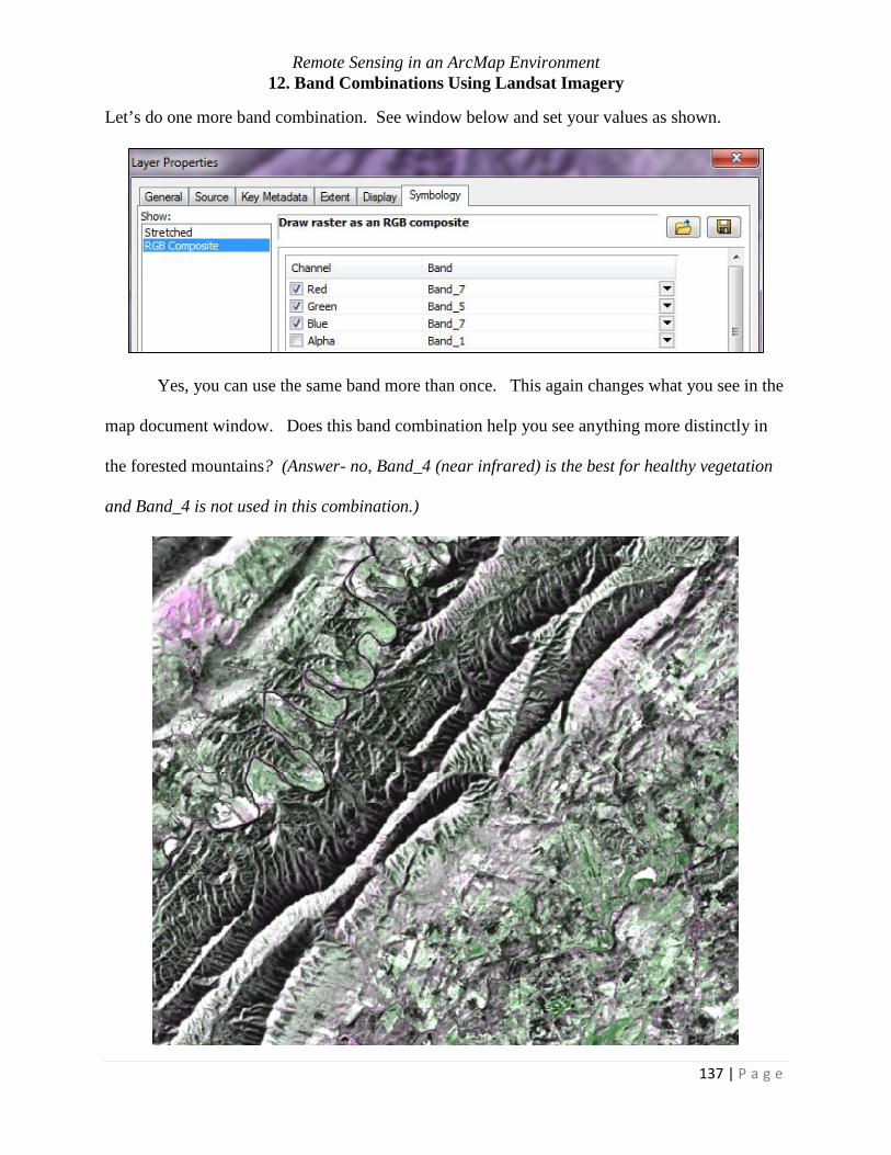
Let’s do one more band combination. See window below and set your values as shown.

Yes, you can use the same band more than once. This again changes what you see in the

map document window. Does this band combination help you see anything more distinctly in

the forested mountains? (Answer- no, Band_4 (near infrared) is the best for healthy vegetation

and Band_4 is not used in this combination.)

137 | P a g e


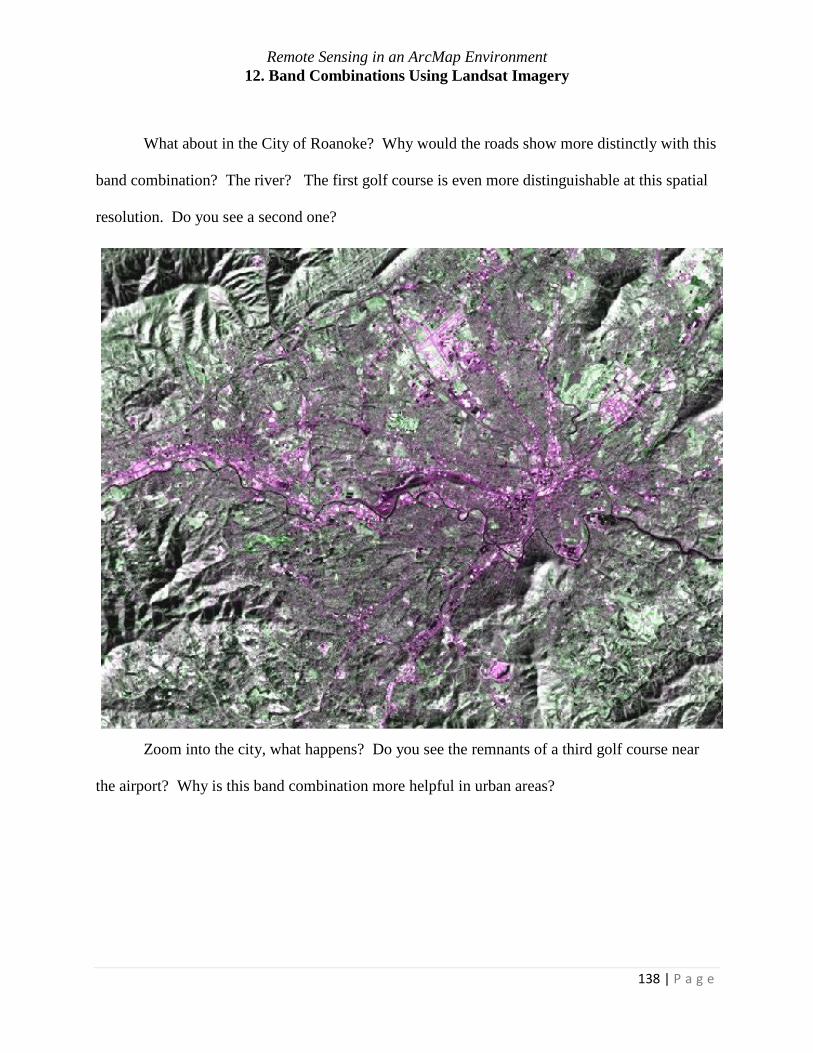
What about in the City of Roanoke? Why would the roads show more distinctly with this

band combination? The river? The first golf course is even more distinguishable at this spatial

resolution. Do you see a second one?

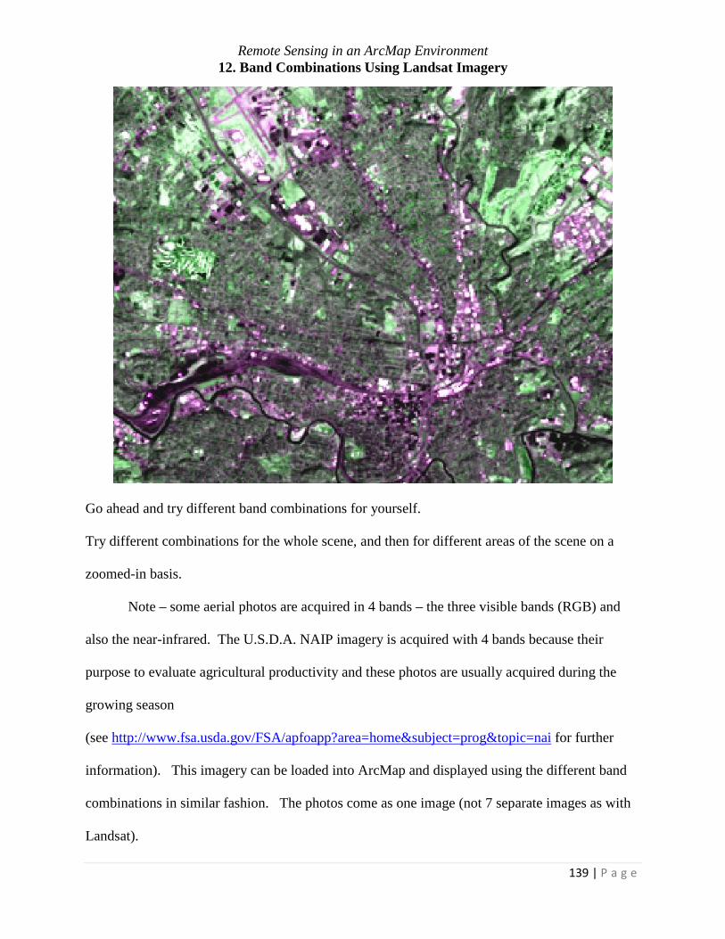
Zoom into the city, what happens? Do you see the remnants of a third golf course near

the airport? Why is this band combination more helpful in urban areas?

138 | P a g e


Go ahead and try different band combinations for yourself.

Try different combinations for the whole scene, and then for different areas of the scene on a

zoomed-in basis.

Note – some aerial photos are acquired in 4 bands – the three visible bands (RGB) and

also the near-infrared. The U.S.D.A. NAIP imagery is acquired with 4 bands because their

purpose to evaluate agricultural productivity and these photos are usually acquired during the

growing season

(see http://www.fsa.usda.gov/FSA/apfoapp?area=home&subject=prog&topic=nai for further

information). This imagery can be loaded into ArcMap and displayed using the different band

combinations in similar fashion. The photos come as one image (not 7 separate images as with

Landsat).

139 | P a g e

http://www.fsa.usda.gov/FSA/apfoapp?area=home&subject=prog&topic=nai


Additional Notes on LANDSAT TM – Single Band Sensitivities 0.45-0.52 μm BLUE (BAND 1) • Shorter wavelengths most sensitive to atmospheric haze and so images may lack tonal

contrast • Shorter wavelengths have greatest water penetration (longer wavelengths more

absorbed); optimal for detection of submerged aquatic vegetation (SAV), pollution plumes, water turbidity and sediment

• Detecting smoke plumes (shorter wavelengths more easily scattered by smaller particles • Good for distinguishing clouds from snow and rock, and soil surfaces from vegetated

surfaces 0.52-0.6 μm GREEN (BAND 2) • Sensitive to water turbidity differences, sediment and pollution plumes • Covers green reflectance peak from leaf surfaces, can be useful for discriminating broad

vegetation classes • Also useful for detection of SAV • Also useful for penetration of water for detection of SAV, pollution plumes, turbidity and

sediment 0.63-0.69 μm RED (BAND 3) • Senses in strong chlorophyll absorption region, i.e. good for discriminating soil and

vegetation • Senses in strong reflectance region for most soils • Delineating soil cover 0.76-0.9 μm NEAR IR (BAND 4) • Distinguishes vegetation varieties and vegetation vigor • Water is strong absorber of NIR, so this band is good for delineation of water bodies and

distinguishing dry and moist soils 1.55-1.75 μm MID OR SWIR (BAND 5) • Sensitive to changes in leaf-tissue water content (turgidity) • Sensitive to moisture variation in vegetation and soils; reflectance decreases as water

content increases • Useful for determining plant vigor and for distinguishing succulents vs. woody vegetation • Especially sensitive to presence/absence of ferric iron or hemitite rocks (reflectance

increases as ferric iron increases) • Discriminates between snow and ice (light toned) and clouds (dark toned) 2.08-2.35 μm MID OR SWIR (BAND 7) • Coincides with absorption band caused by hydrous minerals (clay mica, some oxides, and

sulfates) making them appear darker; e.g. clay alteration zones associated with mineral deposits such as copper

• Lithologic mapping • Like band 5, sensitive to moisture variation in vegetation and soils

140 | P a g e


10.4-12.5 μm LWIR, THERMAL (BAND 6) • Sensor designed to measure radiant surface temps -100 degrees C to +150 degrees C; day

or nighttime use • Heat mapping applications: soil moisture, rock types, thermal water plumes, household

heat conservation, urban heat generation, active military targeting, wildlife inventory, geothermal detection

LANDSAT TM – Band Combination Sensititivies 3-2-1 This combination simulates a natural color image. It is sometimes used for coastal studies and for the detection of smoke plumes. 4-5-3 Used for the analysis of soil moisture and vegetation conditions. It is also good for the location of inland water bodies and land-water boundaries. 4-3-2 Known as false-color Infrared; this is the most conventional band combination used in remote sensing for vegetation, crops, land-use and wetlands analysis. 7-4-2 Analysis of soil and vegetation moisture content and the location of inland water. Vegetation appears green. 5-4-3 Separation of urban and rural land uses; identification of land/water boundaries. 4-5-7 Detection of clouds, snow, and ice (in high latitudes especially).

You are now ready to proceed to the next set of tutorials. We recommend that you

complete the tutorial on sub-setting before you proceed to the tutorials on analyzing Landsat

imagery.

141 | P a g e


Notes:

142 | P a g e

Documents

Chapter 12: Band Combinations using Landsat Imagery …virginiaview.cnre.vt.edu/tutorial/Chapter_12_Band... · · 2014-10-03Using different band combinations to display your scene