Embed Size (px)
Citation preview
1
Chapter 10:Chapter 10:
BASIC MICRO-LEVEL VALUATION: "DCF" & “NPV”
2
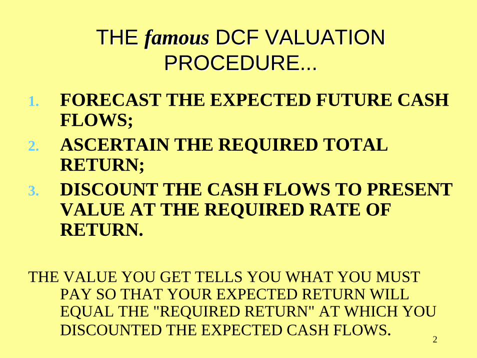
THE THE famousfamous DCF VALUATION DCF VALUATION PROCEDURE...PROCEDURE...
1. FORECAST THE EXPECTED FUTURE CASH FLOWS;
2. ASCERTAIN THE REQUIRED TOTAL RETURN;
3. DISCOUNT THE CASH FLOWS TO PRESENT VALUE AT THE REQUIRED RATE OF RETURN.
THE VALUE YOU GET TELLS YOU WHAT YOU MUST PAY SO THAT YOUR EXPECTED RETURN WILL EQUAL THE "REQUIRED RETURN" AT WHICH YOU DISCOUNTED THE EXPECTED CASH FLOWS.
3
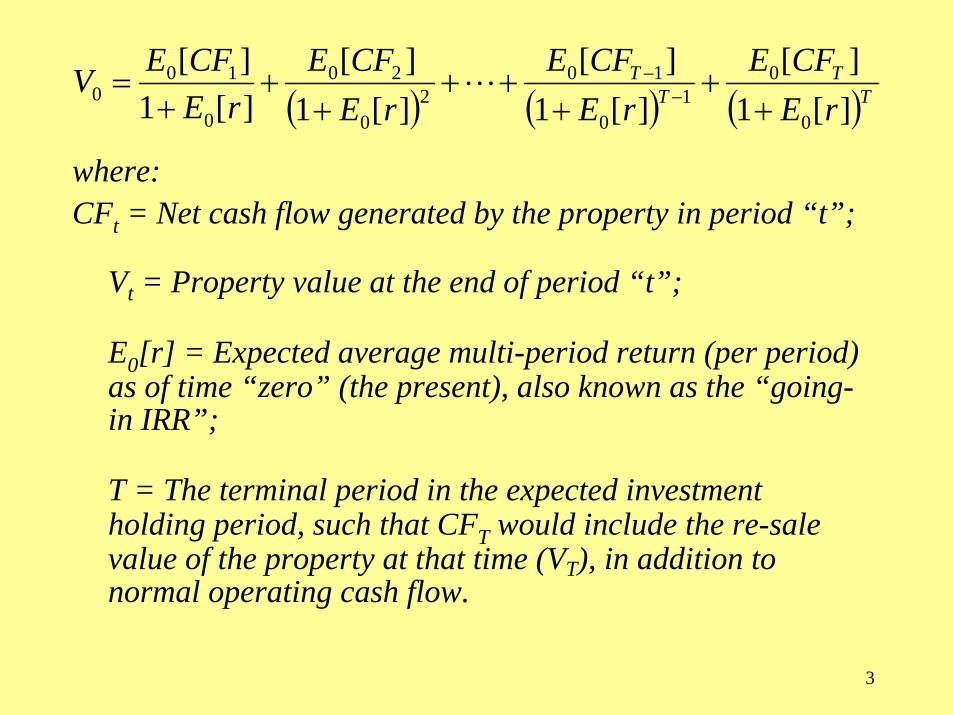
where:CFt = Net cash flow generated by the property in period “t”;
Vt = Property value at the end of period “t”;
E0[r] = Expected average multi-period return (per period) as of time “zero” (the present), also known as the “going-in IRR”;
T = The terminal period in the expected investment holding period, such that CFT would include the re-sale value of the property at that time (VT), in addition to normal operating cash flow.
( ) ( ) ( )TT
TT
rECFE
rECFE
rECFE
rECFEV
][1][
][1][
][1][
][1][
0
01
0
102
0
20
0
100 +
++
+++
++
= −−L
4
Numerical example...Numerical example...
Lease:
Year: CF:
2001 $1,000,000
2002 $1,000,000
2003 $1,000,000
2004 $1,500,000
2005 $1,500,000
2006 $1,500,000
• Single-tenant office bldg• 6-year “net” lease with a “step-up”...• Expected sale price year 6 =
$15,000,000• Required rate of return (“going-in
IRR”) = 10%...• DCF valuation of property is
$15,098,000:
)(1.,000516+
)(1.,00051+
)(1.,00051+
)(1.0,0001+
)(1.0,0001+
)(1.0,0001 = 1 65432 08
00,08
00,08
00,08
00,08
00,08
00,000,098,5
5
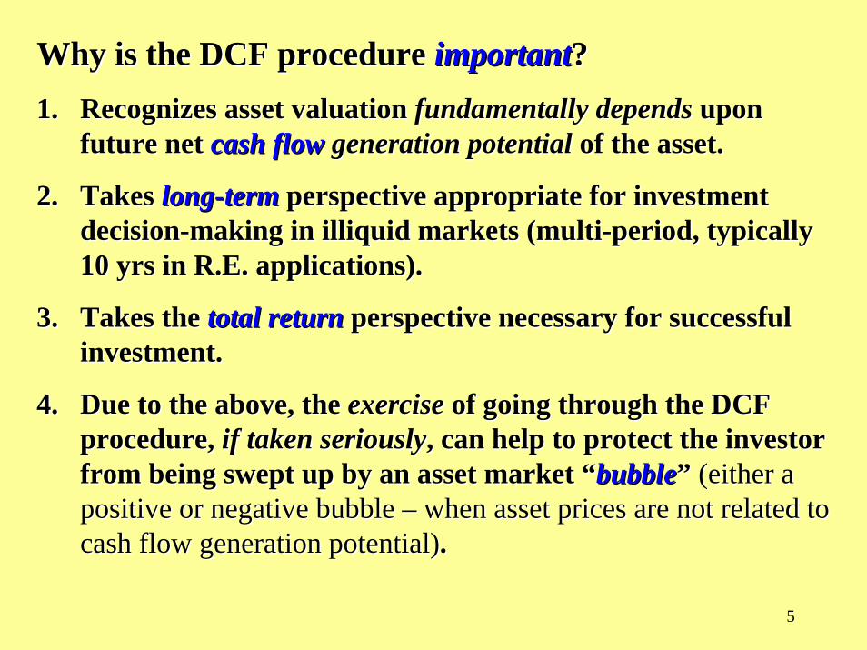
Why is the DCF procedure Why is the DCF procedure importantimportant??1.1. Recognizes asset valuation Recognizes asset valuation fundamentally dependsfundamentally depends upon upon
future net future net cash flowcash flow generation potentialgeneration potential of the asset.of the asset.
2.2. Takes Takes longlong--term term perspective appropriate for investment perspective appropriate for investment decisiondecision--making in illiquid markets (multimaking in illiquid markets (multi--period, typically period, typically 10 yrs in R.E. applications).10 yrs in R.E. applications).
3.3. Takes the Takes the total returntotal return perspective necessary for successful perspective necessary for successful investment.investment.
4.4. Due to the above, the Due to the above, the exerciseexercise of going through the DCF of going through the DCF procedure, procedure, if taken seriouslyif taken seriously, can help to protect the investor , can help to protect the investor from being swept up by an asset market from being swept up by an asset market ““bubblebubble”” (either a (either a positive or negative bubble positive or negative bubble –– when asset prices are not related to when asset prices are not related to cash flow generation potential)cash flow generation potential)..
6
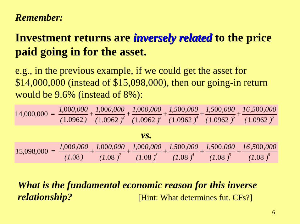
Remember:
Investment returns are inversely relatedinversely related to the price paid going in for the asset.e.g., in the previous example, if we could get the asset for $14,000,000 (instead of $15,098,000), then our going-in return would be 9.6% (instead of 8%):
)(,000516+
)(,00051+
)(,00051+
)(0,0001+
)(0,0001+
)(0,0001 = 65432 0962.1
00,0962.100,
0962.100,
0962.100,
0962.100,
0962.100,000,000,14
vs.
What is the fundamental economic reason for this inverse relationship? [Hint: What determines fut. CFs?]
)(1.,000516+
)(1.,00051+
)(1.,00051+
)(1.0,0001+
)(1.0,0001+
)(1.0,0001 = 1 65432 08
00,08
00,08
00,08
00,08
00,08
00,000,098,5
7
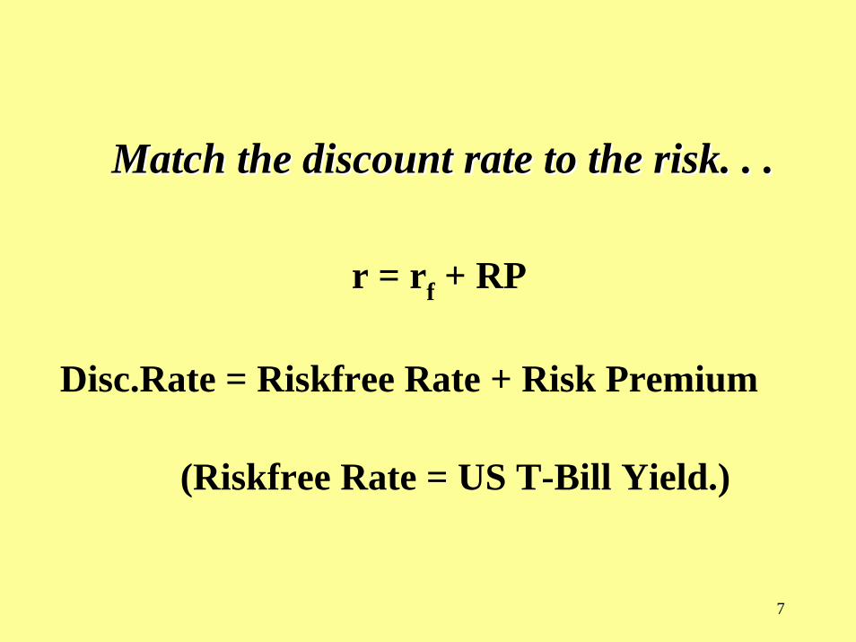
Match the discount rate to the risk. . .Match the discount rate to the risk. . .
r = rf + RP
Disc.Rate = Riskfree Rate + Risk Premium
(Riskfree Rate = US T-Bill Yield.)
8
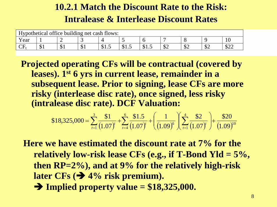
Projected operating CFs will be contractual (covered by leases). 1st 6 yrs in current lease, remainder in a subsequent lease. Prior to signing, lease CFs are more risky (interlease disc rate), once signed, less risky (intralease disc rate). DCF Valuation:
Hypothetical office building net cash flows: Year 1 2 3 4 5 6 7 8 9 10 CFt $1 $1 $1 $1.5 $1.5 $1.5 $2 $2 $2 $22
Here we have estimated the discount rate at 7% for the relatively low-risk lease CFs (e.g., if T-Bond Yld = 5%, then RP=2%), and at 9% for the relatively high-risk later CFs ( 4% risk premium).
Implied property value = $18,325,000.
10.2.1 Match the Discount Rate to the Risk:10.2.1 Match the Discount Rate to the Risk:IntraleaseIntralease & & InterleaseInterlease Discount RatesDiscount Rates
( ) ( ) ( ) ( ) ( )10
4
1
6
46
3
1 09.120$
07.12$
09.11
07.15.1$
07.11$000,325,18$ +⎟⎟
⎠
⎞⎜⎜⎝
⎛⎟⎟⎠
⎞⎜⎜⎝
⎛++= ∑∑∑
=== tt
tt
tt
9
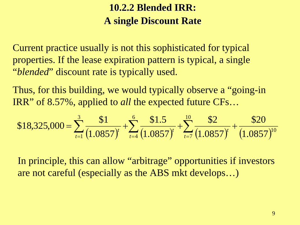
Current practice usually is not this sophisticated for typical properties. If the lease expiration pattern is typical, a single“blended” discount rate is typically used.
Thus, for this building, we would typically observe a “going-in IRR” of 8.57%, applied to all the expected future CFs…
( ) ( ) ( ) ( )10
10
7
6
4
3
1 0857.120$
0857.12$
0857.15.1$
0857.11$000,325,18$ ∑∑∑
===
+++=t
tt
tt
t
In principle, this can allow “arbitrage” opportunities if investors are not careful (especially as the ABS mkt develops…)
10.2.2 Blended IRR:10.2.2 Blended IRR:A single Discount RateA single Discount Rate
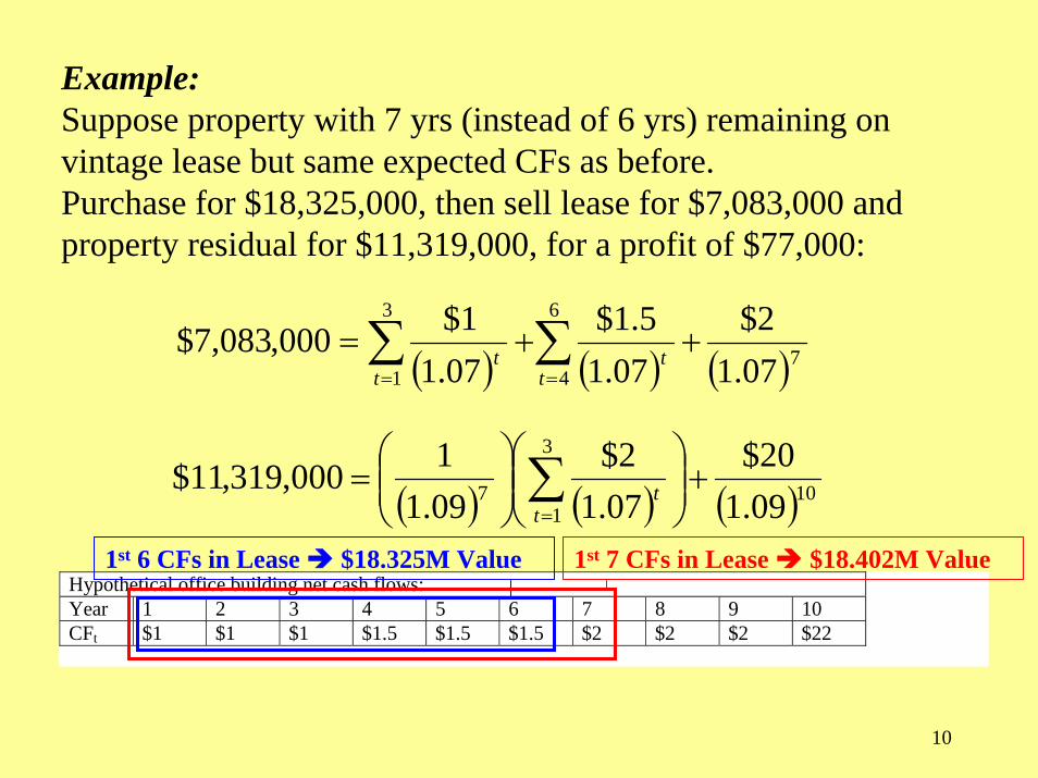
10
Example:Suppose property with 7 yrs (instead of 6 yrs) remaining on vintage lease but same expected CFs as before.Purchase for $18,325,000, then sell lease for $7,083,000 and property residual for $11,319,000, for a profit of $77,000:
( ) ( ) ( )10
3
17 09.1
20$07.12$
09.11000,319,11$ +⎟⎟
⎠
⎞⎜⎜⎝
⎛⎟⎟⎠
⎞⎜⎜⎝
⎛= ∑
=tt
Hypothetical office building net cash flows: Year 1 2 3 4 5 6 7 8 9 10 CFt $1 $1 $1 $1.5 $1.5 $1.5 $2 $2 $2 $22
1st 6 CFs in Lease $18.325M Value 1st 7 CFs in Lease $18.402M Value
( ) ( ) ( )7
6
4
3
1 07.12$
07.15.1$
07.11$000,083,7$ ∑∑
==
++=t
tt
t
11
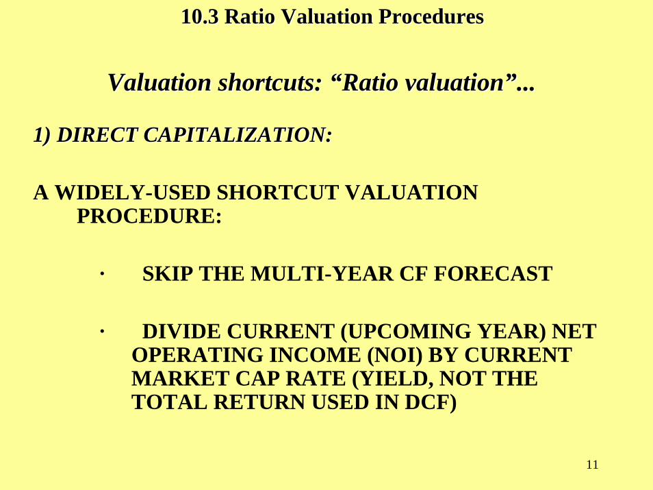
Valuation shortcuts: Valuation shortcuts: ““Ratio valuationRatio valuation””......
1) DIRECT CAPITALIZATION:1) DIRECT CAPITALIZATION:
A WIDELY-USED SHORTCUT VALUATION PROCEDURE:
· SKIP THE MULTI-YEAR CF FORECAST
· DIVIDE CURRENT (UPCOMING YEAR) NET OPERATING INCOME (NOI) BY CURRENT MARKET CAP RATE (YIELD, NOT THE TOTAL RETURN USED IN DCF)
10.3 Ratio Valuation Procedures10.3 Ratio Valuation Procedures
12
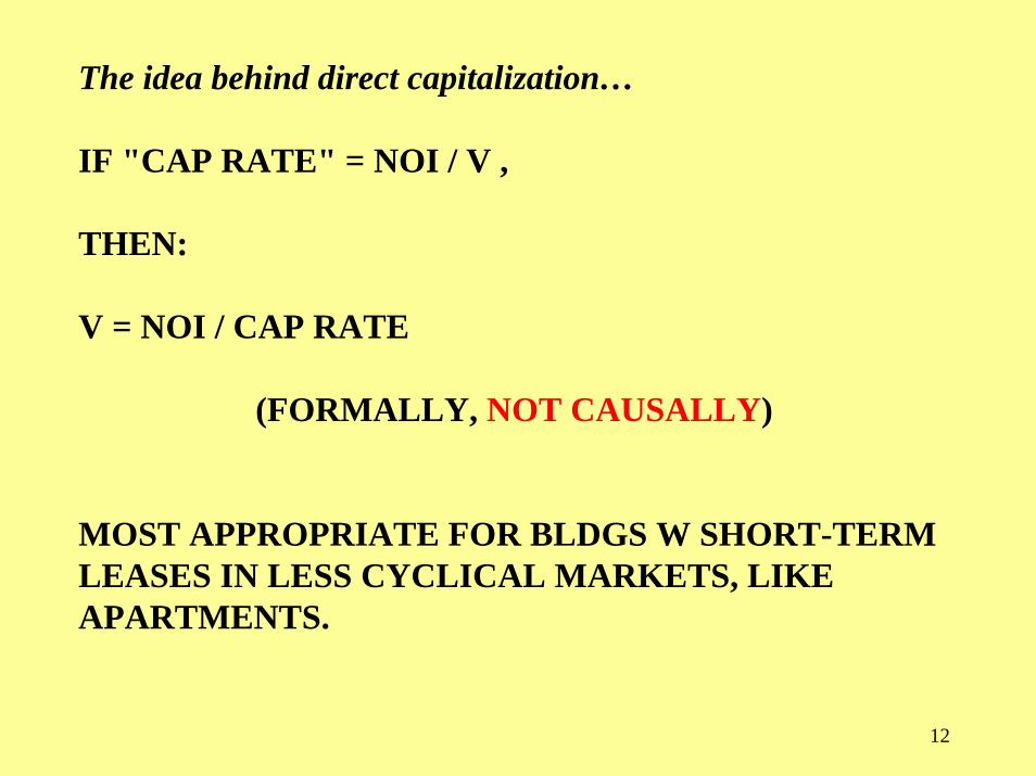
The idea behind direct capitalization…
IF "CAP RATE" = NOI / V ,
THEN:
V = NOI / CAP RATE
(FORMALLY, NOT CAUSALLY)
MOST APPROPRIATE FOR BLDGS W SHORT-TERM LEASES IN LESS CYCLICAL MARKETS, LIKE APARTMENTS.
13
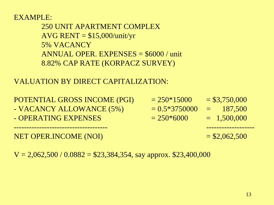
EXAMPLE:250 UNIT APARTMENT COMPLEXAVG RENT = $15,000/unit/yr5% VACANCYANNUAL OPER. EXPENSES = $6000 / unit8.82% CAP RATE (KORPACZ SURVEY)
VALUATION BY DIRECT CAPITALIZATION:
POTENTIAL GROSS INCOME (PGI) = 250*15000 = $3,750,000- VACANCY ALLOWANCE (5%) = 0.5*3750000 = 187,500- OPERATING EXPENSES = 250*6000 = 1,500,000------------------------------------- -------------------NET OPER.INCOME (NOI) = $2,062,500
V = 2,062,500 / 0.0882 = $23,384,354, say approx. $23,400,000
14
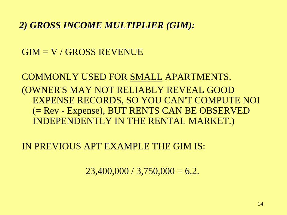
2) GROSS INCOME MULTIPLIER (GIM):2) GROSS INCOME MULTIPLIER (GIM):
GIM = V / GROSS REVENUE
COMMONLY USED FOR SMALL APARTMENTS. (OWNER'S MAY NOT RELIABLY REVEAL GOOD
EXPENSE RECORDS, SO YOU CAN'T COMPUTE NOI (= Rev - Expense), BUT RENTS CAN BE OBSERVED INDEPENDENTLY IN THE RENTAL MARKET.)
IN PREVIOUS APT EXAMPLE THE GIM IS:
23,400,000 / 3,750,000 = 6.2.
15
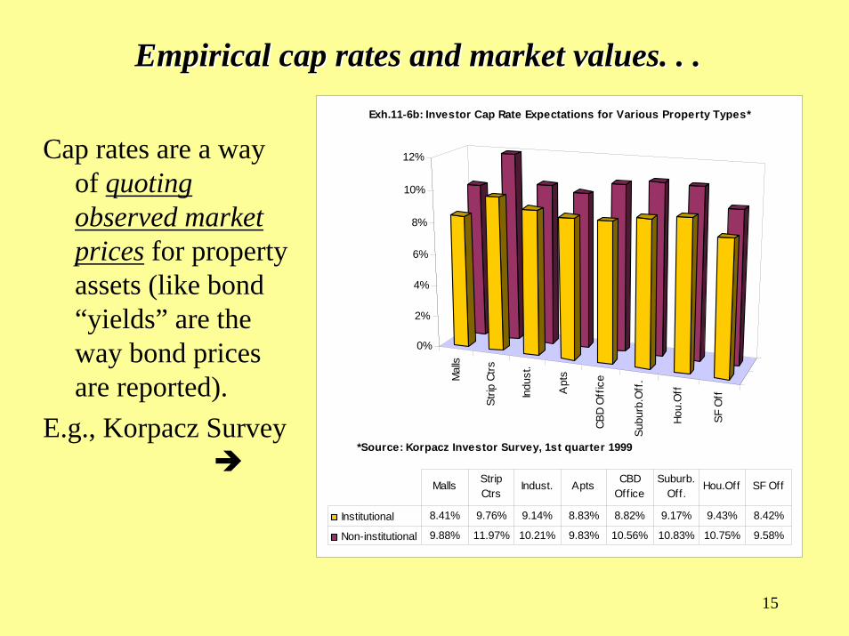
Empirical cap rates and market values. . .Empirical cap rates and market values. . .
Cap rates are a way of quoting observed market prices for property assets (like bond “yields” are the way bond prices are reported).
E.g., Korpacz Survey M
alls
Strip
Ctrs
Indu
st.
Apt
s
CBD
Off
ice
Subu
rb.O
ff.
Hou.
Off
SF O
ff
0%
2%
4%
6%
8%
10%
12%
*Source: Korpacz Investor Survey, 1st quarter 1999
Exh.11-6b: Investor Cap Rate Expectations for Various Property Types*
Institutional 8.41% 9.76% 9.14% 8.83% 8.82% 9.17% 9.43% 8.42%
Non-institutional 9.88% 11.97% 10.21% 9.83% 10.56% 10.83% 10.75% 9.58%
Malls Strip Ctrs
Indust. Apts CBD Office
Suburb.Off.
Hou.Off SF Off
16
DANGERS DANGERS IN MKTIN MKT--BASED RATIO VALUATION. . .BASED RATIO VALUATION. . .
1) 1) DIRECT CAPITALIZATION CAN BE MISLEADING FOR MARKET VALUE IF PROPERTY DOES NOT HAVE CASH FLOW GROWTH AND RISK PATTERN TYPICAL OF OTHER PROPERTIES FROM WHICH CAP RATE WAS OBTAINED. (WITH GIM IT’S EVEN MORE DANGEROUS: OPERATING EXPENSES MUST ALSO BE TYPICAL.)
2) 2) Market-based ratio valuation won’t protect you from “bubbles”!
17
10.4 Typical mistakes in DCF application to 10.4 Typical mistakes in DCF application to commercial property...commercial property...
CAVEAT!BEWARE OF “G.I.G.O.”===> Forecasted Cash Flows:
Must Be REALISTIC Expectations(Neither Optimistic, Nor Pessimistic)
===> Discount Rate should be OCC:Based on Ex Ante Total Returns in Capital Market(Including REALISTIC Property Market Expectations)
· Read the “fine print”.· Look for “hidden assumptions”.· Check realism of assumptions.
18
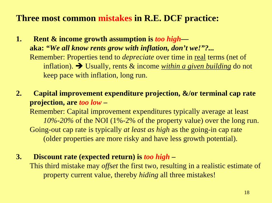
Three most common mistakes in R.E. DCF practice:
1. Rent & income growth assumption is too high—aka: “We all know rents grow with inflation, don’t we!”?... Remember: Properties tend to depreciate over time in real terms (net of
inflation). Usually, rents & income within a given building do not keep pace with inflation, long run.
2. Capital improvement expenditure projection, &/or terminal cap rate projection, are too low –Remember: Capital improvement expenditures typically average at least
10%-20% of the NOI (1%-2% of the property value) over the long run.Going-out cap rate is typically at least as high as the going-in cap rate
(older properties are more risky and have less growth potential).
3. Discount rate (expected return) is too high –This third mistake may offset the first two, resulting in a realistic estimate of
property current value, thereby hiding all three mistakes!
19
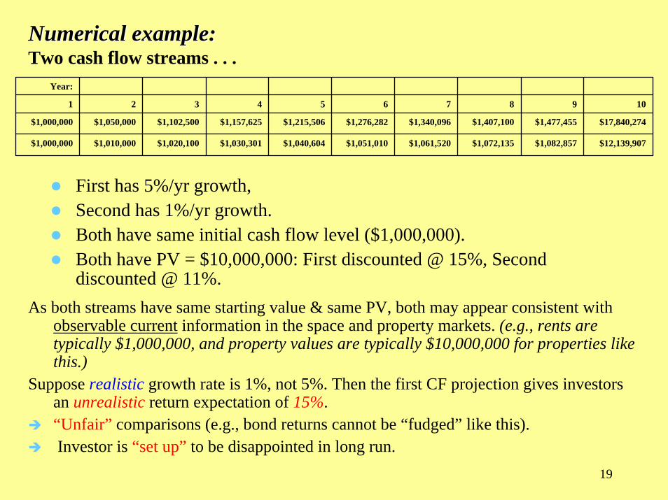
Numerical example:Numerical example:Two cash flow streams . . .
First has 5%/yr growth,Second has 1%/yr growth.Both have same initial cash flow level ($1,000,000).Both have PV = $10,000,000: First discounted @ 15%, Second discounted @ 11%.
Year:
1 2 3 4 5 6 7 8 9 10
$1,000,000 $1,050,000 $1,102,500 $1,157,625 $1,215,506 $1,276,282 $1,340,096 $1,407,100 $1,477,455 $17,840,274
$1,000,000 $1,010,000 $1,020,100 $1,030,301 $1,040,604 $1,051,010 $1,061,520 $1,072,135 $1,082,857 $12,139,907
As both streams have same starting value & same PV, both may appear consistent with observable current information in the space and property markets. (e.g., rents are typically $1,000,000, and property values are typically $10,000,000 for properties like this.)
Suppose realistic growth rate is 1%, not 5%. Then the first CF projection gives investors an unrealistic return expectation of 15%.“Unfair” comparisons (e.g., bond returns cannot be “fudged” like this).Investor is “set up” to be disappointed in long run.
20
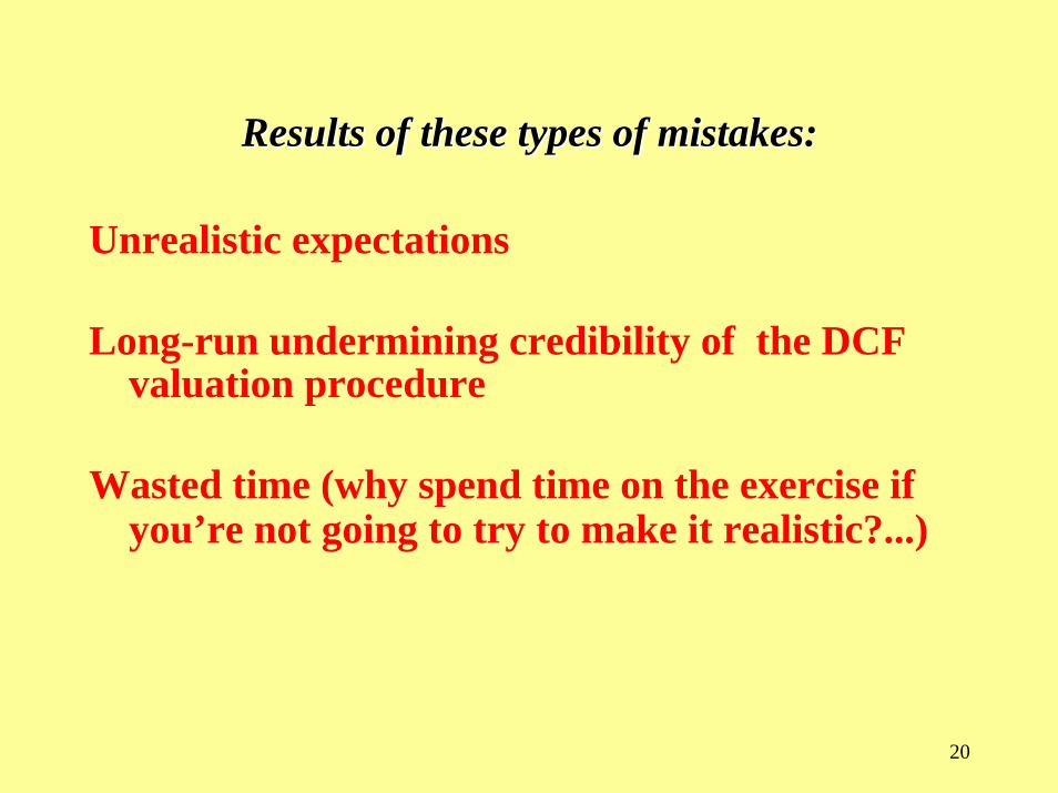
Results of these types of mistakes:Results of these types of mistakes:
Unrealistic expectations
Long-run undermining credibility of the DCF valuation procedure
Wasted time (why spend time on the exercise if you’re not going to try to make it realistic?...)
21
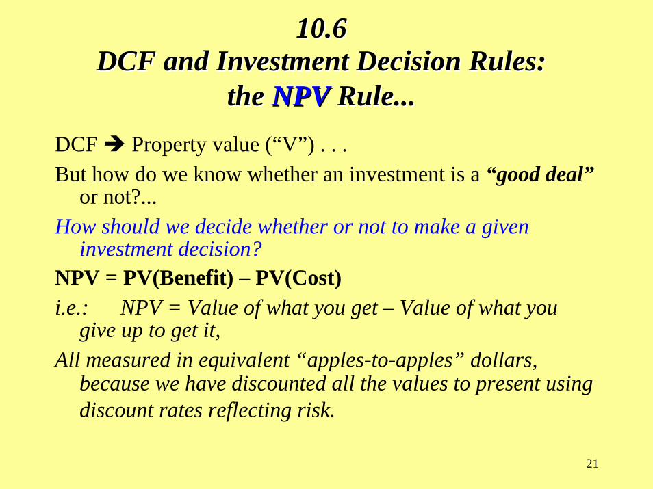
10.610.6DCF and Investment Decision Rules:DCF and Investment Decision Rules:
the the NPVNPV Rule...Rule...DCF Property value (“V”) . . .But how do we know whether an investment is a “good deal”
or not?...How should we decide whether or not to make a given
investment decision?NPV = PV(Benefit) – PV(Cost)i.e.: NPV = Value of what you get – Value of what you
give up to get it,All measured in equivalent “apples-to-apples” dollars,
because we have discounted all the values to present using discount rates reflecting risk.
22
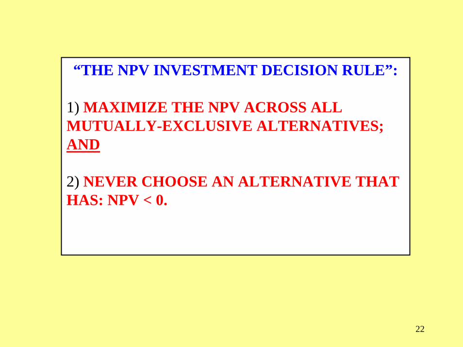
“THE NPV INVESTMENT DECISION RULE”:
1) MAXIMIZE THE NPV ACROSS ALL MUTUALLY-EXCLUSIVE ALTERNATIVES; AND
2) NEVER CHOOSE AN ALTERNATIVE THAT HAS: NPV < 0.
23
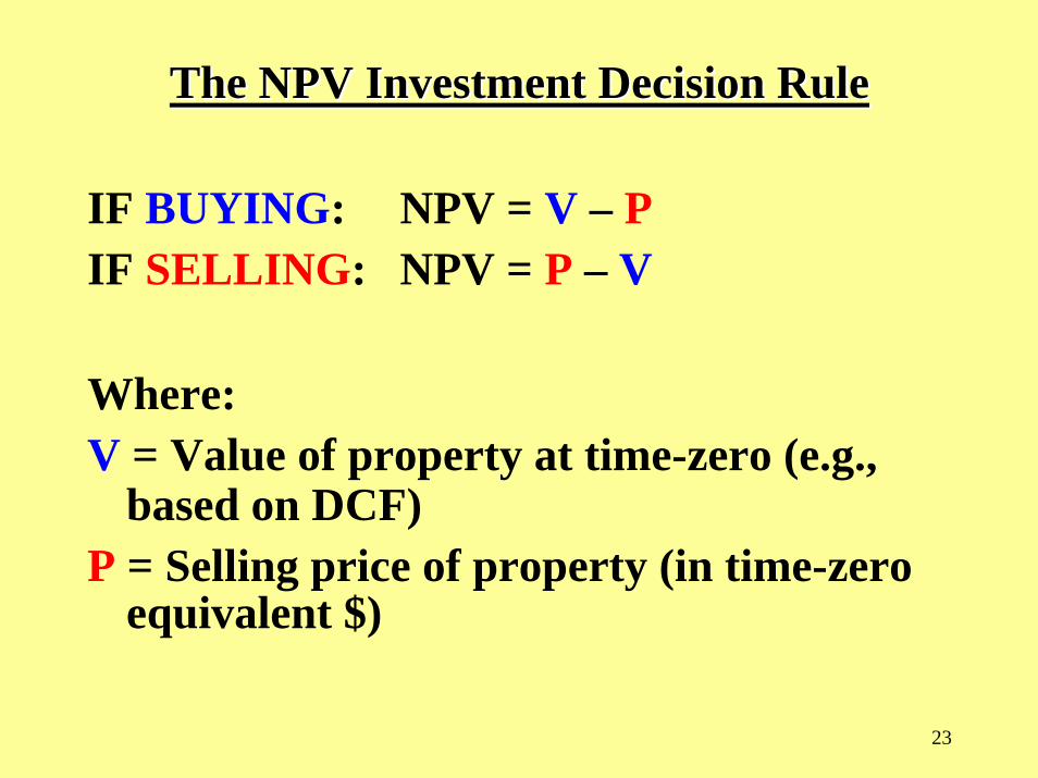
The NPV Investment Decision RuleThe NPV Investment Decision Rule
IF BUYING: NPV = V – PIF SELLING: NPV = P – V
Where:V = Value of property at time-zero (e.g.,
based on DCF)P = Selling price of property (in time-zero
equivalent $)
24
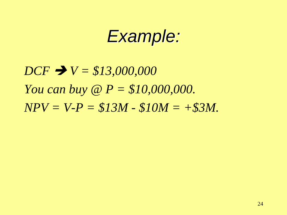
Example:Example:
DCF V = $13,000,000You can buy @ P = $10,000,000.NPV = V-P = $13M - $10M = +$3M.
25
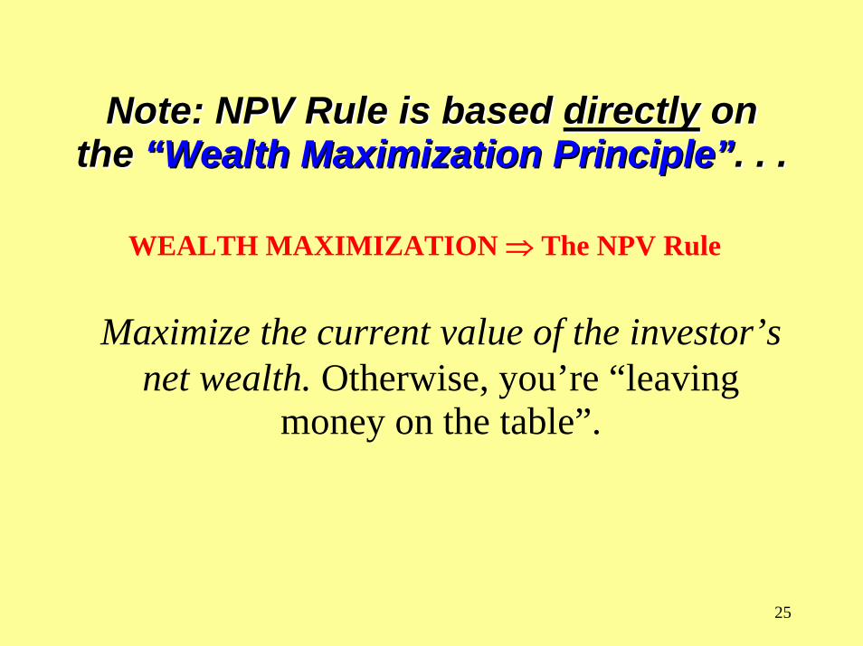
Note: NPV Rule is based Note: NPV Rule is based directlydirectly on on the the ““Wealth Maximization PrincipleWealth Maximization Principle””. . .. . .
WEALTH MAXIMIZATION ⇒ The NPV Rule
Maximize the current value of the investor’s net wealth. Otherwise, you’re “leaving
money on the table”.
26
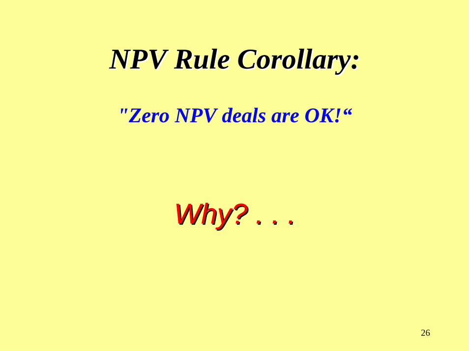
NPV Rule Corollary:NPV Rule Corollary:
"Zero NPV deals are OK!“
Why? . . .Why? . . .
27
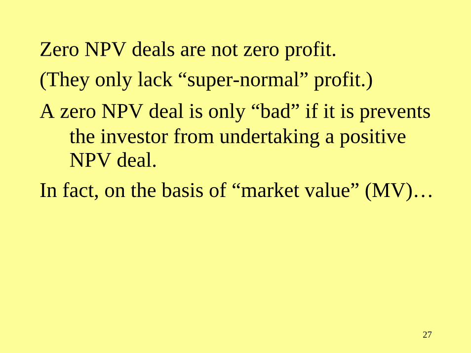
Zero NPV deals are not zero profit.(They only lack “super-normal” profit.)A zero NPV deal is only “bad” if it is prevents
the investor from undertaking a positive NPV deal.
In fact, on the basis of “market value” (MV)…
28
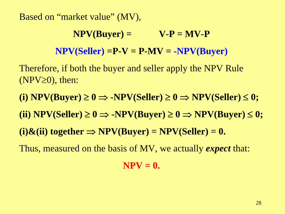
Based on “market value” (MV),
NPV(Buyer) = V-P = MV-P
NPV(Seller) =P-V = P-MV = -NPV(Buyer)
Therefore, if both the buyer and seller apply the NPV Rule (NPV≥0), then:
(i) NPV(Buyer) ≥ 0 ⇒ -NPV(Seller) ≥ 0 ⇒ NPV(Seller) ≤ 0;
(ii) NPV(Seller) ≥ 0 ⇒ -NPV(Buyer) ≥ 0 ⇒ NPV(Buyer) ≤ 0;
(i)&(ii) together ⇒ NPV(Buyer) = NPV(Seller) = 0.
Thus, measured on the basis of MV, we actually expect that:
NPV = 0.
29
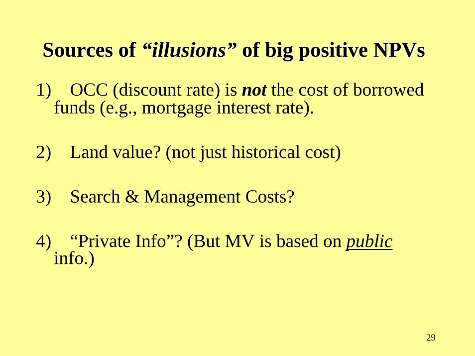
Sources of Sources of ““illusionsillusions”” of big positive of big positive NPVsNPVs
1) OCC (discount rate) is not the cost of borrowed funds (e.g., mortgage interest rate).
2) Land value? (not just historical cost)
3) Search & Management Costs?
4) “Private Info”? (But MV is based on publicinfo.)
30
However, in Real Estate it is possible to However, in Real Estate it is possible to occasionallyoccasionally find deals with substantially find deals with substantially positive, or negative, NPV, even based on MV.positive, or negative, NPV, even based on MV.
Real estate asset markets not informationallyefficient:- People make “pricing mistakes” (they can’t observe MV for sure for a given property)- Your own research may uncover “news”relevant to value (just before the market knows it)
31
What about What about uniqueunique circumstances or abilities? . . .circumstances or abilities? . . .
Generally, real uniqueness does not affect MV.
Precisely because you are unique, you can’t expect someone else to be willing to pay what you could, or be willing to sell for what you would. (May affect “investment value” –IV, not MV.)
32
10.6.2 Choosing Among Alternative Zero10.6.2 Choosing Among Alternative Zero--NPV InvestmentsNPV Investments
• Alternatives may have different NPVs based on “investment value”, even though they all have equal (zero) NPV based on “market value”. (See Sect. 12.1.)
• One alternative may be preferable for macro or strategic reasons (portfolio target, administrative efficiency, property size preference, etc.).
• Alternatives may present different expected return “attributes” (initial yield, cash flow change, yield change). (See Appendix 10B & Sect. 26.1.1.)
33
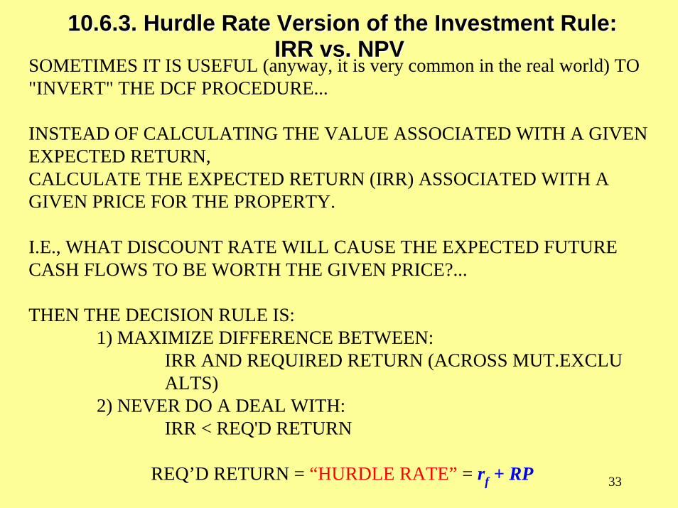
10.6.3. Hurdle Rate Version of the Investment Rule: 10.6.3. Hurdle Rate Version of the Investment Rule: IRR vs. NPVIRR vs. NPV
SOMETIMES IT IS USEFUL (anyway, it is very common in the real world) TO "INVERT" THE DCF PROCEDURE...
INSTEAD OF CALCULATING THE VALUE ASSOCIATED WITH A GIVEN EXPECTED RETURN,CALCULATE THE EXPECTED RETURN (IRR) ASSOCIATED WITH A GIVEN PRICE FOR THE PROPERTY.
I.E., WHAT DISCOUNT RATE WILL CAUSE THE EXPECTED FUTURE CASH FLOWS TO BE WORTH THE GIVEN PRICE?...
THEN THE DECISION RULE IS:1) MAXIMIZE DIFFERENCE BETWEEN:
IRR AND REQUIRED RETURN (ACROSS MUT.EXCLU ALTS)
2) NEVER DO A DEAL WITH:IRR < REQ'D RETURN
REQ’D RETURN = “HURDLE RATE” = rf + RP
34
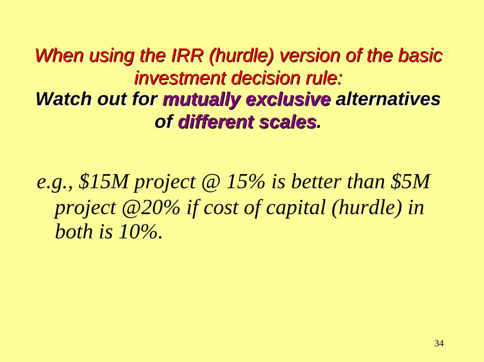
When using the IRR (hurdle) version of the basic When using the IRR (hurdle) version of the basic investment decision rule:investment decision rule:
Watch out for Watch out for mutually exclusivemutually exclusive alternativesalternativesof of different scalesdifferent scales..
e.g., $15M project @ 15% is better than $5M project @20% if cost of capital (hurdle) in both is 10%.
35
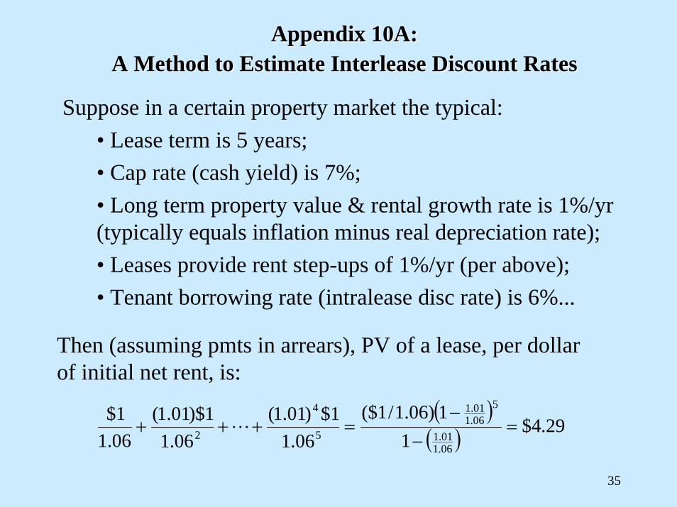
Appendix 10A: Appendix 10A: A Method to Estimate A Method to Estimate InterleaseInterlease Discount RatesDiscount Rates
Suppose in a certain property market the typical:• Lease term is 5 years;• Cap rate (cash yield) is 7%;• Long term property value & rental growth rate is 1%/yr (typically equals inflation minus real depreciation rate);• Leases provide rent step-ups of 1%/yr (per above);• Tenant borrowing rate (intralease disc rate) is 6%...
( )( ) 29.4$
11)06.1/1($
06.11$)01.1(
06.11)$01.1(
06.11$
06.101.1
506.101.1
5
4
2 =−
−=+++ L
Then (assuming pmts in arrears), PV of a lease, per dollar of initial net rent, is:
36
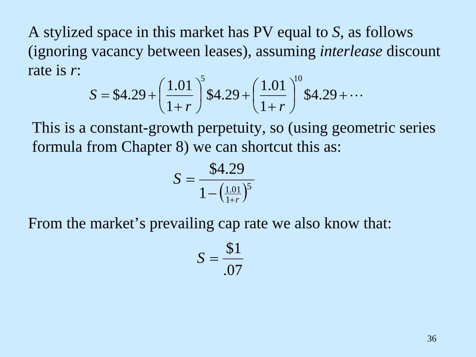
L+⎟⎠⎞
⎜⎝⎛+
+⎟⎠⎞
⎜⎝⎛+
+= 29.4$1
01.129.4$1
01.129.4$105
rrS
A stylized space in this market has PV equal to S, as follows (ignoring vacancy between leases), assuming interlease discount rate is r:
( )5101.1129.4$
r
S+−
=
This is a constant-growth perpetuity, so (using geometric series formula from Chapter 8) we can shortcut this as:
From the market’s prevailing cap rate we also know that:
07.1$
=S
37
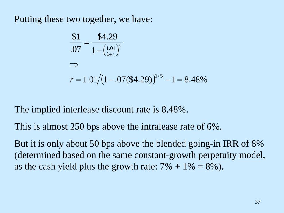
Putting these two together, we have:
( )
( ) %48.81)29.4($07.101.1
129.4$
07.1$
5/1
51
01.1
=−−=
⇒
−=
+
r
r
The implied interlease discount rate is 8.48%.
This is almost 250 bps above the intralease rate of 6%.
But it is only about 50 bps above the blended going-in IRR of 8% (determined based on the same constant-growth perpetuity model, as the cash yield plus the growth rate: 7% + 1% = 8%).
38
Appendix 10B (& Ch.26 Sect. 26.1.1)Appendix 10B (& Ch.26 Sect. 26.1.1)
PropertyProperty--LevelLevelInvestment Performance Investment Performance
AttributionAttribution
39
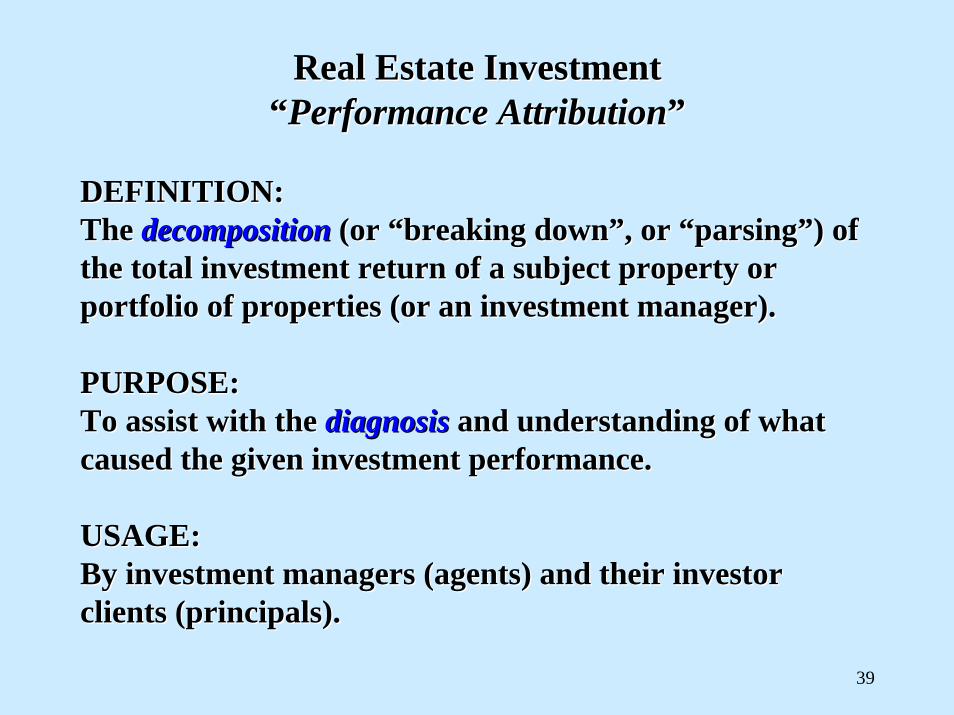
Real Estate InvestmentReal Estate Investment““Performance AttributionPerformance Attribution””
DEFINITION: DEFINITION: The The decompositiondecomposition (or (or ““breaking downbreaking down””, or , or ““parsingparsing””) of ) of the total investment return of a subject property or the total investment return of a subject property or portfolio of properties (or an investment manager).portfolio of properties (or an investment manager).
PURPOSE:PURPOSE:To assist with the To assist with the diagnosisdiagnosis and understanding of what and understanding of what caused the given investment performance.caused the given investment performance.
USAGE:USAGE:By investment managers (agents) and their investor By investment managers (agents) and their investor clients (principals).clients (principals).
40
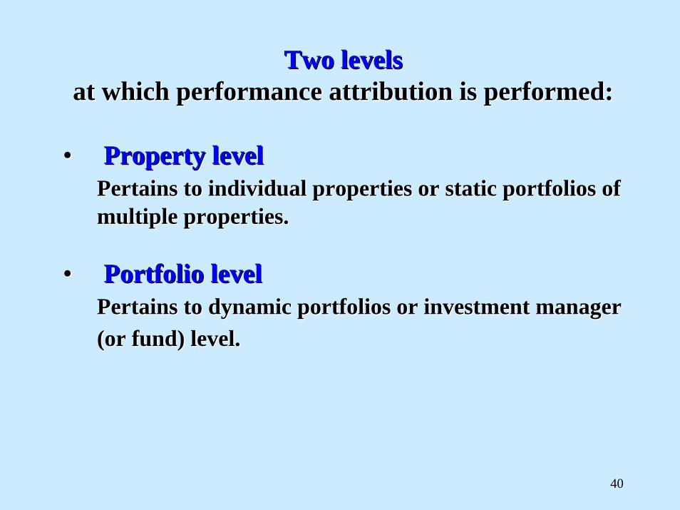
Two levelsTwo levelsat which performance attribution is performed:at which performance attribution is performed:
•• Property levelProperty levelPertains to individual properties or static portfolios of Pertains to individual properties or static portfolios of multiple properties.multiple properties.
•• Portfolio levelPortfolio levelPertains to dynamic portfolios or investment manager Pertains to dynamic portfolios or investment manager (or fund) level.(or fund) level.
41
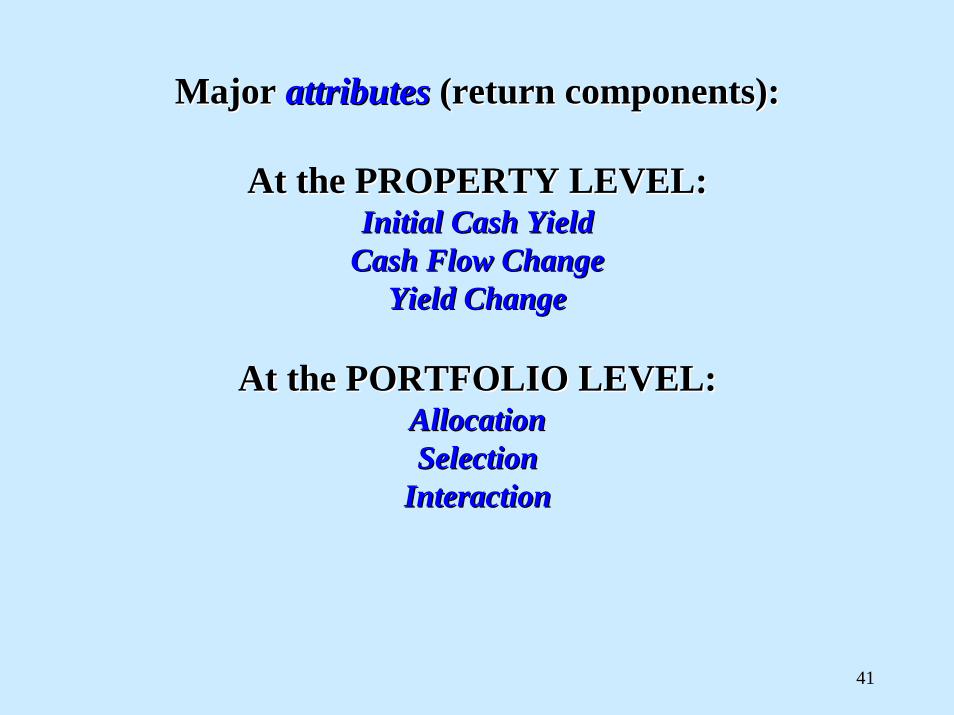
Major Major attributesattributes (return components):(return components):
At the PROPERTY LEVEL:At the PROPERTY LEVEL:Initial Cash YieldInitial Cash Yield
Cash Flow ChangeCash Flow ChangeYield ChangeYield Change
At the PORTFOLIO LEVEL:At the PORTFOLIO LEVEL:AllocationAllocationSelectionSelection
InteractionInteraction
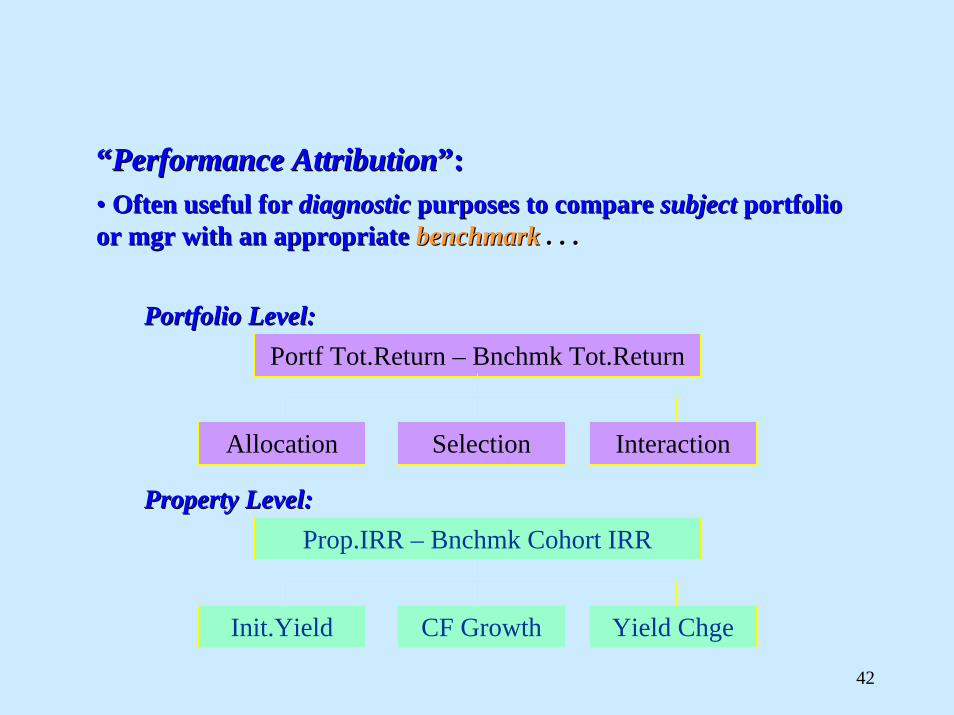
42
““Performance AttributionPerformance Attribution””::
Portf Tot.Return – Bnchmk Tot.Return
Allocation Selection Interaction
Portfolio Level:Portfolio Level:
Prop.IRR – Bnchmk Cohort IRR
Init.Yield CF Growth Yield Chge
Property Level:Property Level:
•• Often useful for Often useful for diagnosticdiagnostic purposes to compare purposes to compare subjectsubject portfolio portfolio or mgr with an appropriateor mgr with an appropriate benchmarkbenchmark . . .. . .
43
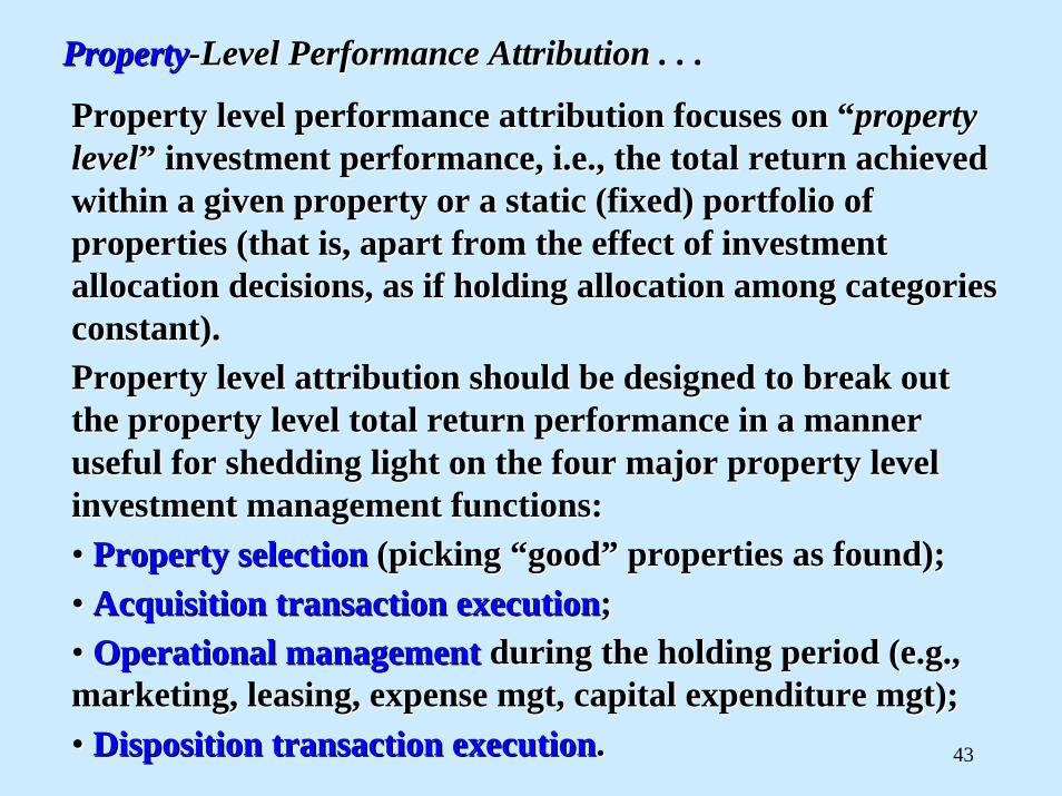
PropertyProperty--Level Performance Attribution Level Performance Attribution . . .. . .
Property level performance attribution focuses on Property level performance attribution focuses on ““property property levellevel”” investment performance, i.e., the total return achieved investment performance, i.e., the total return achieved within a given property or a static (fixed) portfolio of within a given property or a static (fixed) portfolio of properties (that is, apart from the effect of investment properties (that is, apart from the effect of investment allocation decisions, as if holding allocation among categories allocation decisions, as if holding allocation among categories constant).constant).Property level attribution should be designed to break out Property level attribution should be designed to break out the property level total return performance in a manner the property level total return performance in a manner useful for shedding light on the four major property level useful for shedding light on the four major property level investment management functions:investment management functions:•• Property selectionProperty selection (picking (picking ““goodgood”” properties as found);properties as found);•• Acquisition transaction executionAcquisition transaction execution;;•• Operational managementOperational management during the holding period (e.g., during the holding period (e.g., marketing, leasing, expense mgt, capital expenditure mgt);marketing, leasing, expense mgt, capital expenditure mgt);•• Disposition transaction executionDisposition transaction execution..
44
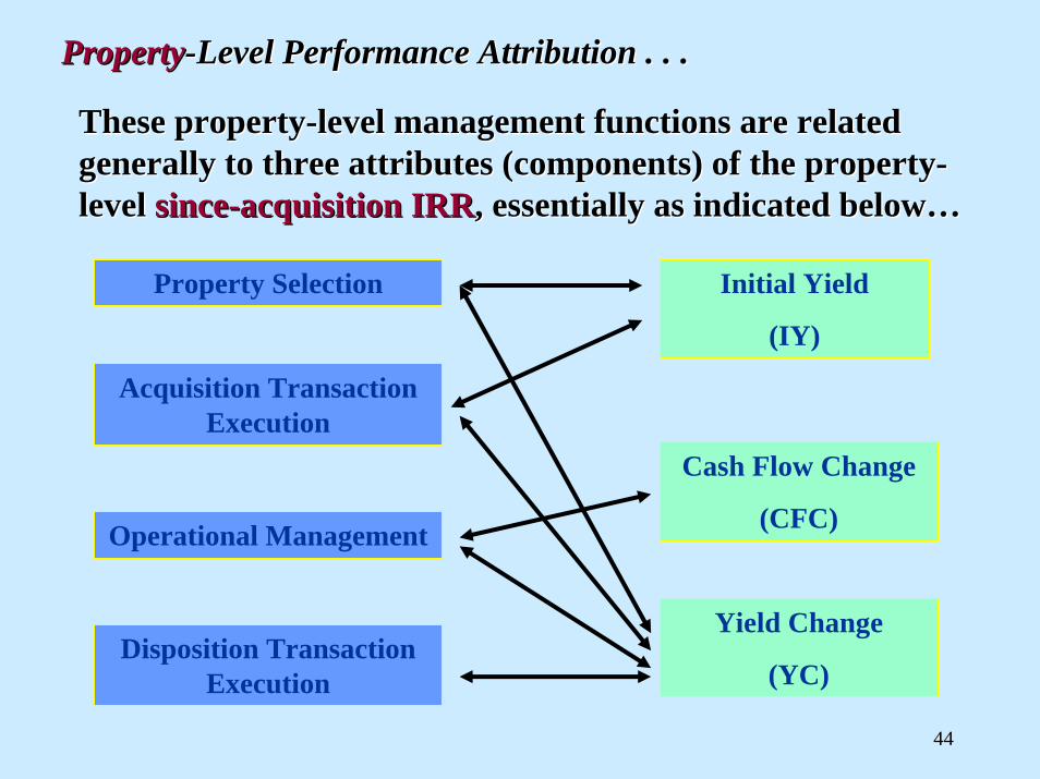
PropertyProperty--Level Performance Attribution Level Performance Attribution . . .. . .
These propertyThese property--level management functions are related level management functions are related generally to three attributes (components) of the propertygenerally to three attributes (components) of the property--level level sincesince--acquisition IRRacquisition IRR, essentially as indicated below, essentially as indicated below……
Initial Yield
(IY)
Cash Flow Change
(CFC)
Yield Change
(YC)
Property Selection
Acquisition Transaction Execution
Operational Management
Disposition Transaction Execution
45
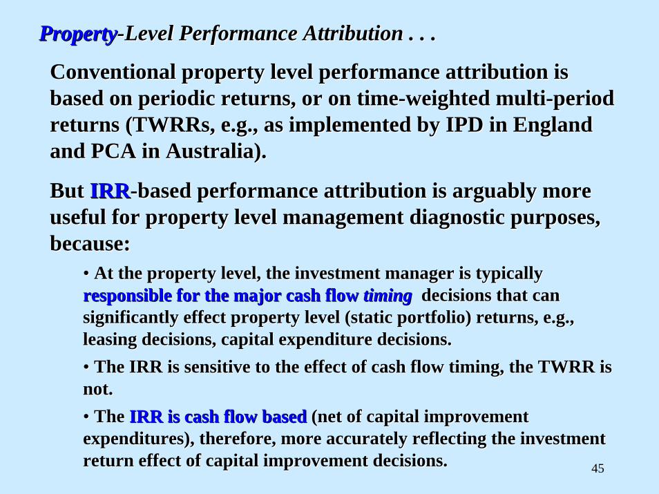
Conventional property level performance attribution is Conventional property level performance attribution is based on periodic returns, or on timebased on periodic returns, or on time--weighted multiweighted multi--period period returns (returns (TWRRsTWRRs, e.g., as implemented by IPD in England , e.g., as implemented by IPD in England and PCA in Australia).and PCA in Australia).
But But IRRIRR--based performance attribution is arguably more based performance attribution is arguably more useful for property level management diagnostic purposes, useful for property level management diagnostic purposes, because:because:
•• At the property level, the investment manager is typically At the property level, the investment manager is typically responsible for the major cash flow responsible for the major cash flow timingtiming decisions that can decisions that can significantly effect property level (static portfolio) returns, significantly effect property level (static portfolio) returns, e.g., e.g., leasing decisions, capital expenditure decisions.leasing decisions, capital expenditure decisions.•• The IRR is sensitive to the effect of cash flow timing, the TWRThe IRR is sensitive to the effect of cash flow timing, the TWRR is R is not.not.•• The The IRR is cash flow basedIRR is cash flow based (net of capital improvement (net of capital improvement expenditures), therefore, more accurately reflecting the investmexpenditures), therefore, more accurately reflecting the investment ent return effect of capital improvement decisions.return effect of capital improvement decisions.
PropertyProperty--Level Performance Attribution Level Performance Attribution . . .. . .
46
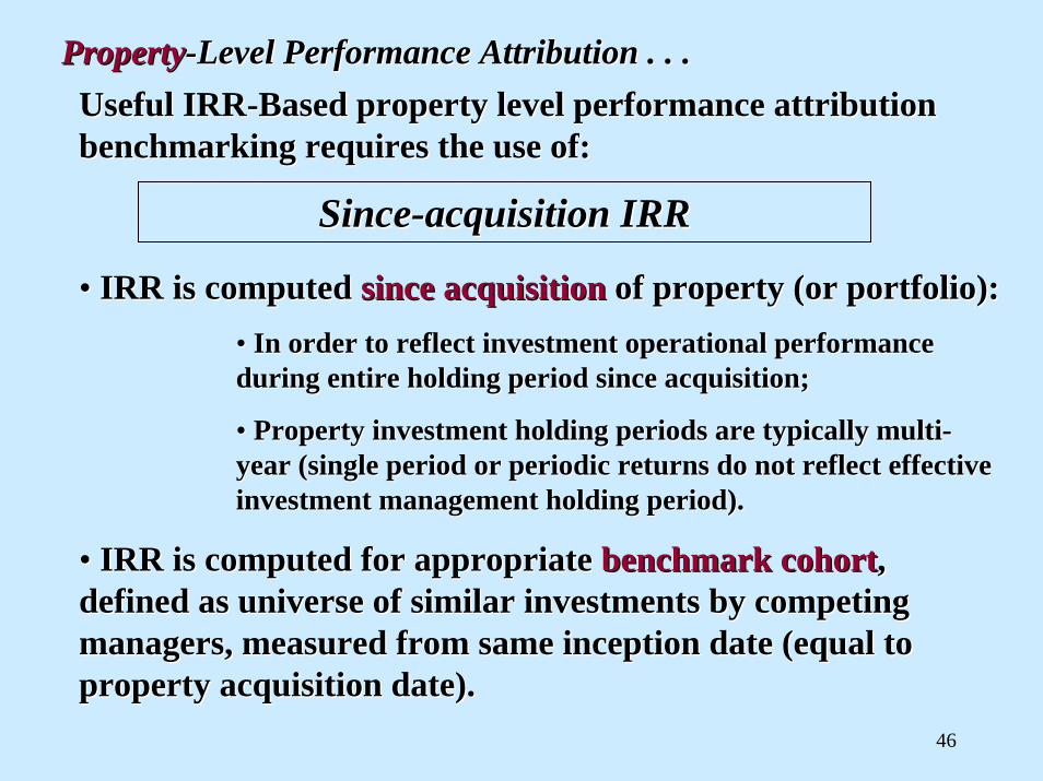
Useful IRRUseful IRR--Based property level performance attribution Based property level performance attribution benchmarking requires the use of:benchmarking requires the use of:
SinceSince--acquisition IRRacquisition IRR
•• IRR is computed IRR is computed since acquisitionsince acquisition of property (or portfolio):of property (or portfolio):•• In order to reflect investment operational performance In order to reflect investment operational performance during entire holding period since acquisition;during entire holding period since acquisition;
•• Property investment holding periods are typically multiProperty investment holding periods are typically multi--year (single period or periodic returns do not reflect effectiveyear (single period or periodic returns do not reflect effectiveinvestment management holding period).investment management holding period).
•• IRR is computed for appropriate IRR is computed for appropriate benchmark cohortbenchmark cohort, , defined as universe of similar investments by competing defined as universe of similar investments by competing managers, measured from same inception date (equal to managers, measured from same inception date (equal to property acquisition date).property acquisition date).
PropertyProperty--Level Performance Attribution Level Performance Attribution . . .. . .
47
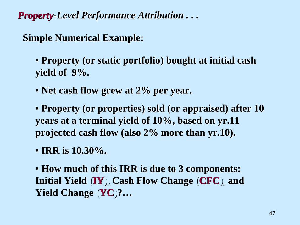
Simple Numerical Example:Simple Numerical Example:
•• Property (or static portfolio) bought at initial cash Property (or static portfolio) bought at initial cash yield of 9%.yield of 9%.
•• Net cash flow grew at 2% per year.Net cash flow grew at 2% per year.
•• Property (or properties) sold (or appraised) after 10 Property (or properties) sold (or appraised) after 10 years at a terminal yield of 10%, based on yr.11 years at a terminal yield of 10%, based on yr.11 projected cash flow (also 2% more than yr.10).projected cash flow (also 2% more than yr.10).
•• IRR is 10.30%.IRR is 10.30%.
•• How much of this IRR is due to 3 components: How much of this IRR is due to 3 components: Initial Yield Initial Yield ((IYIY),), Cash Flow Change Cash Flow Change ((CFCCFC),), and and Yield Change Yield Change ((YCYC))??……
PropertyProperty--Level Performance Attribution Level Performance Attribution . . .. . .
48
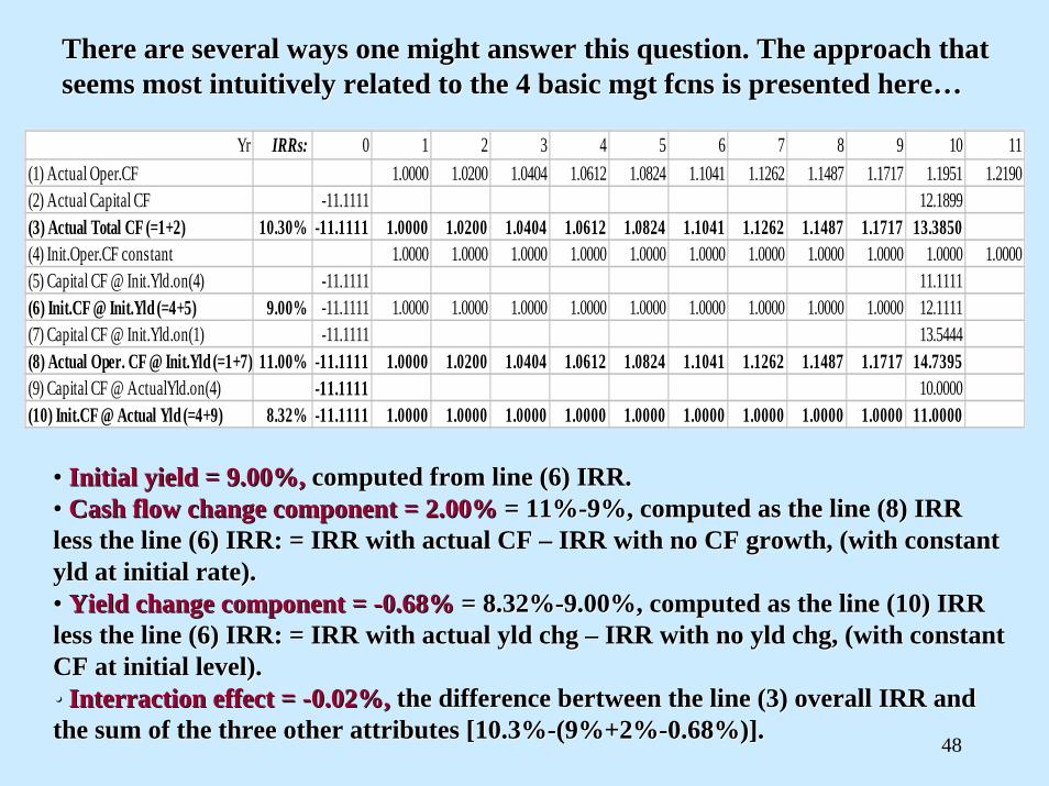
Yr IRRs: 0 1 2 3 4 5 6 7 8 9 10 11(1) Actual Oper.CF 1.0000 1.0200 1.0404 1.0612 1.0824 1.1041 1.1262 1.1487 1.1717 1.1951 1.2190(2) Actual Capital CF -11.1111 12.1899(3) Actual Total CF (=1+2) 10.30% -11.1111 1.0000 1.0200 1.0404 1.0612 1.0824 1.1041 1.1262 1.1487 1.1717 13.3850(4) Init.Oper.CF constant 1.0000 1.0000 1.0000 1.0000 1.0000 1.0000 1.0000 1.0000 1.0000 1.0000 1.0000(5) Capital CF @ Init.Yld.on(4) -11.1111 11.1111(6) Init.CF @ Init.Yld (=4+5) 9.00% -11.1111 1.0000 1.0000 1.0000 1.0000 1.0000 1.0000 1.0000 1.0000 1.0000 12.1111(7) Capital CF @ Init.Yld.on(1) -11.1111 13.5444(8) Actual Oper. CF @ Init.Yld (=1+7) 11.00% -11.1111 1.0000 1.0200 1.0404 1.0612 1.0824 1.1041 1.1262 1.1487 1.1717 14.7395(9) Capital CF @ ActualYld.on(4) -11.1111 10.0000(10) Init.CF @ Actual Yld (=4+9) 8.32% -11.1111 1.0000 1.0000 1.0000 1.0000 1.0000 1.0000 1.0000 1.0000 1.0000 11.0000
There are several ways one might answer this question. The approThere are several ways one might answer this question. The approach that ach that seems most intuitively related to the 4 basic mgt seems most intuitively related to the 4 basic mgt fcnsfcns is presented hereis presented here……
•• Initial yield = 9.00%,Initial yield = 9.00%, computed from line (6) IRR.computed from line (6) IRR.•• Cash flow change component = 2.00%Cash flow change component = 2.00% = 11%= 11%--9%, computed as the line (8) IRR 9%, computed as the line (8) IRR less the line (6) IRR: = IRR with actual CF less the line (6) IRR: = IRR with actual CF –– IRR with no CF growth, (with constant IRR with no CF growth, (with constant yldyld at initial rate).at initial rate).•• Yield change component = Yield change component = --0.68%0.68% = 8.32%= 8.32%--9.00%, computed as the line (10) IRR 9.00%, computed as the line (10) IRR less the line (6) IRR: = IRR with actual less the line (6) IRR: = IRR with actual yldyld chg chg –– IRR with no IRR with no yldyld chg, (with constant chg, (with constant CF at initial level).CF at initial level).•• InterractionInterraction effect = effect = --0.02%,0.02%, the difference the difference bertweenbertween the line (3) overall IRR and the line (3) overall IRR and the sum of the three other attributes [10.3%the sum of the three other attributes [10.3%--(9%+2%(9%+2%--0.68%)].0.68%)].
49
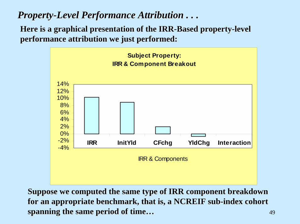
PropertyProperty--Level Performance Attribution Level Performance Attribution . . .. . .
Subject Property: IRR & Component Breakout
-4%-2%0%2%4%6%8%
10%12%14%
IRR InitYld CFchg YldChg Interaction
IRR & Components
Here is a graphical presentation of the IRRHere is a graphical presentation of the IRR--Based propertyBased property--level level performance attribution we just performed:performance attribution we just performed:
Suppose we computed the same type of IRR component breakdown Suppose we computed the same type of IRR component breakdown for an appropriate benchmark, that is, a NCREIF subfor an appropriate benchmark, that is, a NCREIF sub--index cohort index cohort spanning the same period of timespanning the same period of time……
50
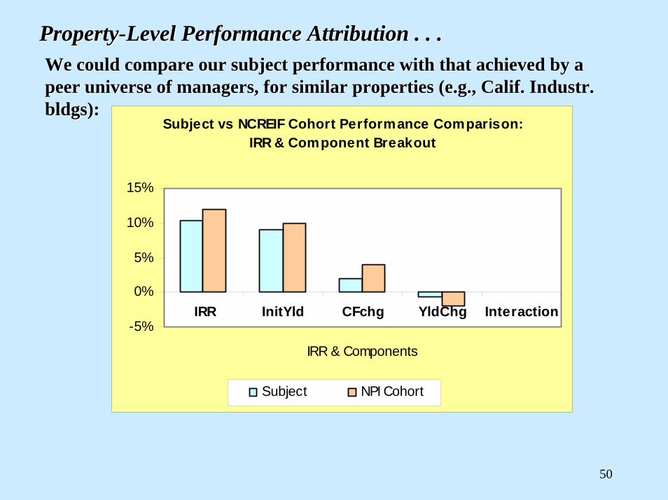
PropertyProperty--Level Performance Attribution Level Performance Attribution . . .. . .We could compare our subject performance with that achieved by aWe could compare our subject performance with that achieved by apeer universe of managers, for similar properties (e.g., Calif. peer universe of managers, for similar properties (e.g., Calif. IndustrIndustr. . bldgsbldgs):):
Subject vs NCREIF Cohort Performance Comparison: IRR & Component Breakout
-5%
0%
5%
10%
15%
IRR InitYld CFchg YldChg Interaction
IRR & Components
Subject NPI Cohort
51
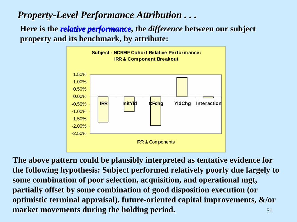
PropertyProperty--Level Performance Attribution Level Performance Attribution . . .. . .Here is the Here is the relative performancerelative performance, the , the differencedifference between our subject between our subject property and its benchmark, by attribute:property and its benchmark, by attribute:
The above pattern could be plausibly interpreted as tentative evThe above pattern could be plausibly interpreted as tentative evidence for idence for the following hypothesis: Subject performed relatively poorly duthe following hypothesis: Subject performed relatively poorly due largely to e largely to some combination of poor selection, acquisition, and operationalsome combination of poor selection, acquisition, and operational mgt, mgt, partially offset by some combination of good disposition executipartially offset by some combination of good disposition execution (or on (or optimistic terminal appraisal), futureoptimistic terminal appraisal), future--oriented capital improvements, &/or oriented capital improvements, &/or market movements during the holding period.market movements during the holding period.
Subject - NCREIF Cohort Relative Performance: IRR & Component Breakout
-2.50%-2.00%-1.50%-1.00%-0.50%0.00%0.50%1.00%1.50%
IRR InitYld CFchg YldChg Interaction
IRR & Components
52
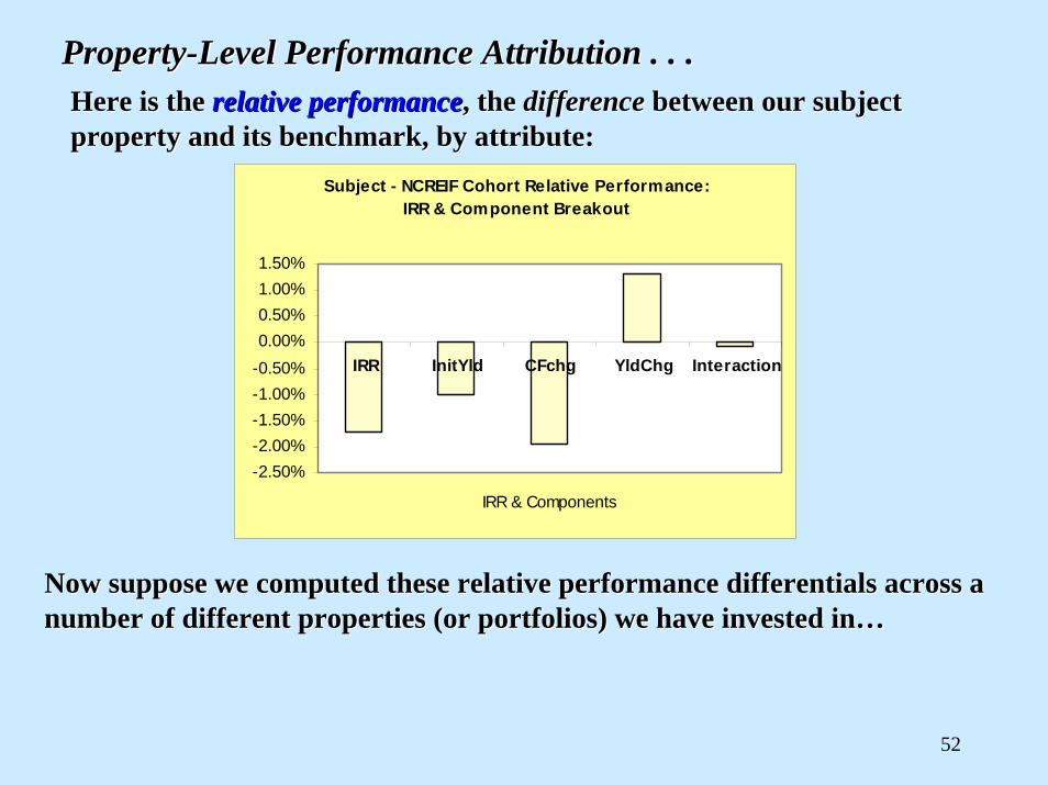
PropertyProperty--Level Performance Attribution Level Performance Attribution . . .. . .Here is the Here is the relative performancerelative performance, the , the differencedifference between our subject between our subject property and its benchmark, by attribute:property and its benchmark, by attribute:
Now suppose we computed these relative performance differentialsNow suppose we computed these relative performance differentials across a across a number of different properties (or portfolios) we have invested number of different properties (or portfolios) we have invested inin……
Subject - NCREIF Cohort Relative Performance: IRR & Component Breakout
-2.50%-2.00%-1.50%-1.00%-0.50%0.00%0.50%1.00%1.50%
IRR InitYld CFchg YldChg Interaction
IRR & Components
53
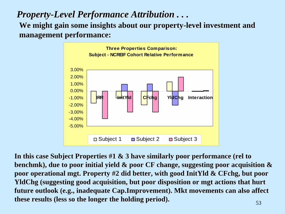
PropertyProperty--Level Performance Attribution Level Performance Attribution . . .. . .We might gain some insights about our propertyWe might gain some insights about our property--level investment and level investment and management performance:management performance:
In this case Subject Properties #1 & 3 have similarly poor perfoIn this case Subject Properties #1 & 3 have similarly poor performance (rmance (relrel to to benchmkbenchmk), due to poor initial yield & poor CF change, suggesting poor a), due to poor initial yield & poor CF change, suggesting poor acquisition & cquisition & poor operational mgt. Property #2 did better, with good poor operational mgt. Property #2 did better, with good InitYldInitYld & & CFchgCFchg, but poor , but poor YldChgYldChg (suggesting good acquisition, but poor disposition or mgt actio(suggesting good acquisition, but poor disposition or mgt actions that hurt ns that hurt future outlook (e.g., inadequate Cap.Improvement). future outlook (e.g., inadequate Cap.Improvement). MktMkt movements can also affect movements can also affect these results (less so the longer the holding period).these results (less so the longer the holding period).
Three Properties Comparison:Subject - NCREIF Cohort Relative Performance
-5.00%-4.00%-3.00%-2.00%-1.00%0.00%1.00%2.00%3.00%
IRR InitYld CFchg YldChg Interaction
Subject 1 Subject 2 Subject 3
54
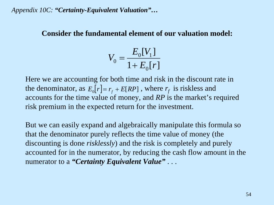
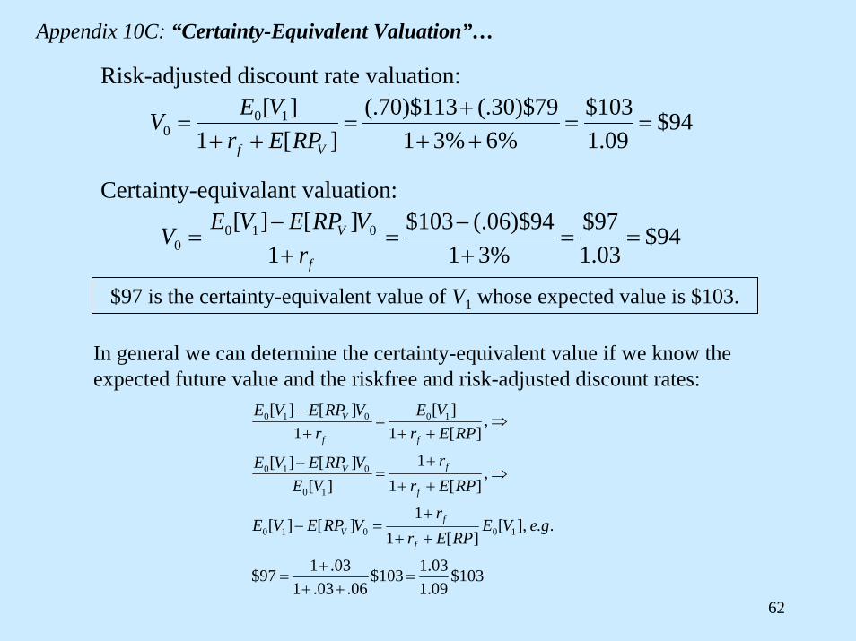
Appendix 10C: “Certainty-Equivalent Valuation”…
Consider the fundamental element of our valuation model:
][1][
0
100 rE
VEV+
=
Here we are accounting for both time and risk in the discount rate in the denominator, as , where rf is riskless and accounts for the time value of money, and RP is the market’s required risk premium in the expected return for the investment.
[ ] ][0 RPErrE f +=
But we can easily expand and algebraically manipulate this formula so that the denominator purely reflects the time value of money (the discounting is done risklessly) and the risk is completely and purely accounted for in the numerator, by reducing the cash flow amount in the numerator to a “Certainty Equivalent Value” . . .
55
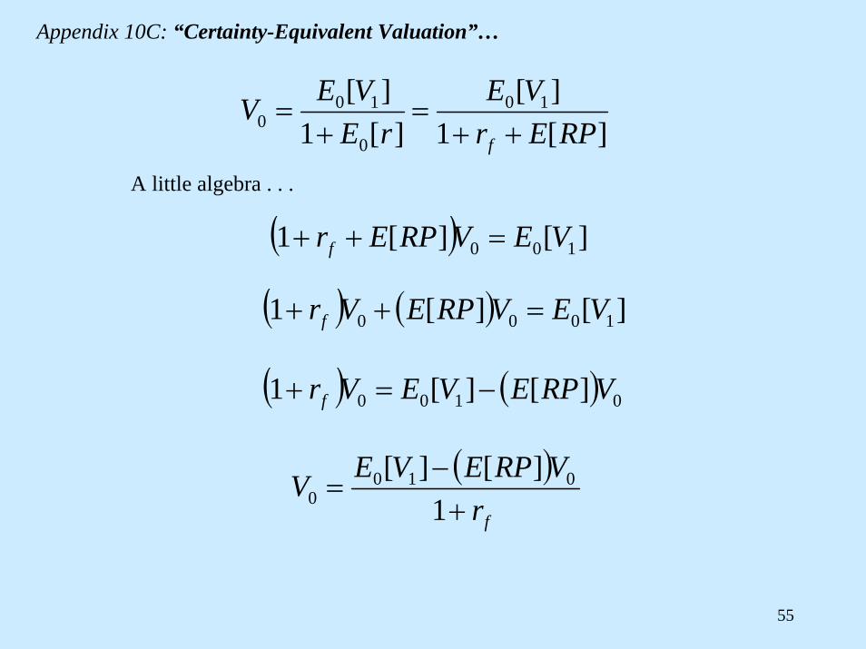
][1][
][1][ 10
0
100 RPEr
VErE
VEVf ++
=+
=
( )fr
VRPEVEV+
−=
1][][ 010
0
( ) ( ) 0100 ][][1 VRPEVEVrf −=+
( ) ( ) ][][1 1000 VEVRPEVrf =++
( ) ][][1 100 VEVRPErf =++
A little algebra . . .
Appendix 10C: “Certainty-Equivalent Valuation”…
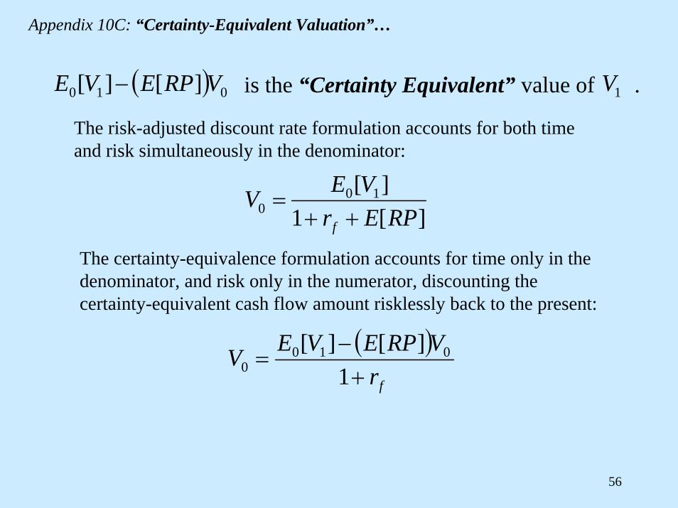
56
][1][ 10
0 RPErVEV
f ++=
( )fr
VRPEVEV+
−=
1][][ 010
0
( ) 010 ][][ VRPEVE − is the “Certainty Equivalent” value of . 1V
The risk-adjusted discount rate formulation accounts for both time and risk simultaneously in the denominator:
The certainty-equivalence formulation accounts for time only in the denominator, and risk only in the numerator, discounting the certainty-equivalent cash flow amount risklessly back to the present:
Appendix 10C: “Certainty-Equivalent Valuation”…
57
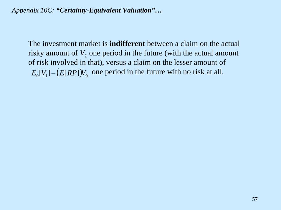
( ) 010 ][][ VRPEVE −
The investment market is indifferent between a claim on the actual risky amount of V1 one period in the future (with the actual amount of risk involved in that), versus a claim on the lesser amount of
one period in the future with no risk at all.
Appendix 10C: “Certainty-Equivalent Valuation”…
58
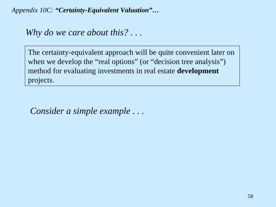
Why do we care about this? . . .
The certainty-equivalent approach will be quite convenient later on when we develop the “real options” (or “decision tree analysis”) method for evaluating investments in real estate developmentprojects.
Consider a simple example . . .
Appendix 10C: “Certainty-Equivalent Valuation”…
59
Suppose:
Riskfree interest rate = 3%
Stock market total return risk premium = 6%
Stock Mkt expected total return is:
E[rS] = rf + E[RPS] = 3% + 6% = 9%
“Binomial World”…
A stock mkt total return index that today has value 1.00 will next year have a value of either:
1.13 (with 70% probability), or
0.79 (with 30% probability).
Therefore, expected value of index next yr is:
E[S1] = (0.70)1.13 + (0.30)0.79 = 1.03
Appendix 10C: “Certainty-Equivalent Valuation”…
60
S = 1.13
S = 0.79
Prob = 70%
Prob = 30%
S0
Here is the situation in the stock market…
Today
Next Year
Appendix 10C: “Certainty-Equivalent Valuation”…
61
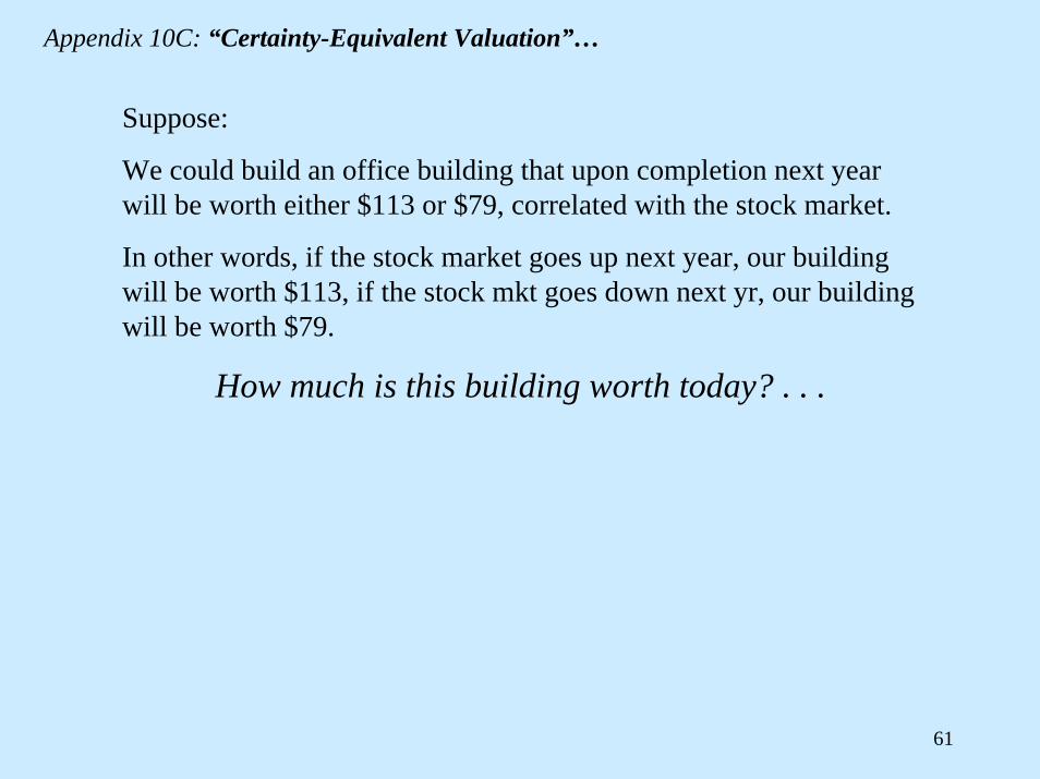
Suppose:
We could build an office building that upon completion next yearwill be worth either $113 or $79, correlated with the stock market.
In other words, if the stock market goes up next year, our building will be worth $113, if the stock mkt goes down next yr, our building will be worth $79.
How much is this building worth today? . . .
Appendix 10C: “Certainty-Equivalent Valuation”…
62
94$09.1
103$%6%31
79)$30(.113)$70(.][1
][ 100 ==
+++
=++
=Vf RPEr
VEV
Risk-adjusted discount rate valuation:
94$03.197$
%3194)$06(.103$
1][][ 010
0 ==+−
=+−
=f
V
rVRPEVEV
Certainty-equivalant valuation:
$97 is the certainty-equivalent value of V1 whose expected value is $103.
In general we can determine the certainty-equivalent value if we know the expected future value and the riskfree and risk-adjusted discount rates:
103$09.103.1103$
06.03.103.197$
..],[][1
1][][
,][1
1][
][][
,][1
][1
][][
10010
10
010
10010
=++
+=
++
+=−
⇒++
+=
−
⇒++
=+−
geVERPEr
rVRPEVE
RPErr
VEVRPEVE
RPErVE
rVRPEVE
f
fV
f
fV
ff
V
Appendix 10C: “Certainty-Equivalent Valuation”…
63
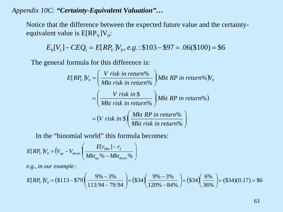
Notice that the difference between the expected future value and the certainty-equivalent value is E[RPV]V0:
6$)100($06.97$103$:..,][][ 0110 ==−=− geVRPECEQVE V
The general formula for this difference is:
( )
( )
( ) ⎟⎟⎠
⎞⎜⎜⎝
⎛=
⎟⎟⎠
⎞⎜⎜⎝
⎛=
⎟⎟⎠
⎞⎜⎜⎝
⎛=
%%$
%%
$
%%
%][ 00
returninriskMktreturninRPMktinriskV
returninRPMktreturninriskMktinriskV
VreturninRPMktreturninriskMkt
returninriskVVRPE V
( )
( ) ( ) ( ) 6$)17.0)(34($%36%634$
%84%120%3%934$
947994113%3%979$113$][
:.,.
%%][
][
0
0
==⎟⎠⎞
⎜⎝⎛=⎟
⎠⎞
⎜⎝⎛
−−
=⎟⎟⎠
⎞⎜⎜⎝
⎛−−
−=
⎟⎟⎠
⎞⎜⎜⎝
⎛
−
−−=
VRPE
exampleouringe
MktMktrrE
VVVRPE
V
downup
fMktdownupV
In the “binomial world” this formula becomes:
Appendix 10C: “Certainty-Equivalent Valuation”…
64
⎟⎟⎠
⎞⎜⎜⎝
⎛==⎟⎟
⎠
⎞⎜⎜⎝
⎛=
][],[""
%%
][][
Mkt
MktV
Mkt
V
rVARrrCOVBeta
returninriskMktreturninriskV
RPERPE
In the “CAPM”:
(Don’t worry about this in this class.)
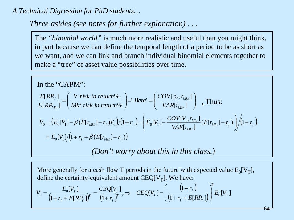
Three asides (see notes for further explanation) . . .
The “binomial world” is much more realistic and useful than you might think, in part because we can define the temporal length of a period to be as short as we want, and we can link and branch individual binomial elements together to make a “tree” of asset value possibilities over time.
, Thus:
( ) ( ) ( )( ))][(1][
1)][(][
],[][1)][(][
10
1100100
fMktf
ffMktMkt
MktffMkt
rrErVE
rrrErVAR
rVCOVVErVrrEVEV
−++=
+⎟⎟⎠
⎞⎜⎜⎝
⎛−−=+−−=
β
β
More generally for a cash flow T periods in the future with expected value E0[VT], define the certainty-equivalent amount CEQ[VT]. We have:
( ) ( )( )
( ) ][][1
1][,
1][
][1][
00
0 T
T
Vf
fTT
f
TT
Vf
T VERPEr
rVCEQ
rVCEQ
RPErVEV ⎟
⎟⎠
⎞⎜⎜⎝
⎛
+++
=⇒+
=++
=
A Technical Digression for PhD students…
65
Let’s go back to our office building example…
Suppose the office building does not exist yet,
but we could build it in 1 year
by paying $90 of construction cost upon completion of construction next year. (Construction is instantaneous: We can decide next year whether to build or not.)
Suppose our option to build this project expires in 1 year: We either build then or we lose the right to ever build.
How much is this option worth?
Appendix 10C: “Certainty-Equivalent Valuation”…
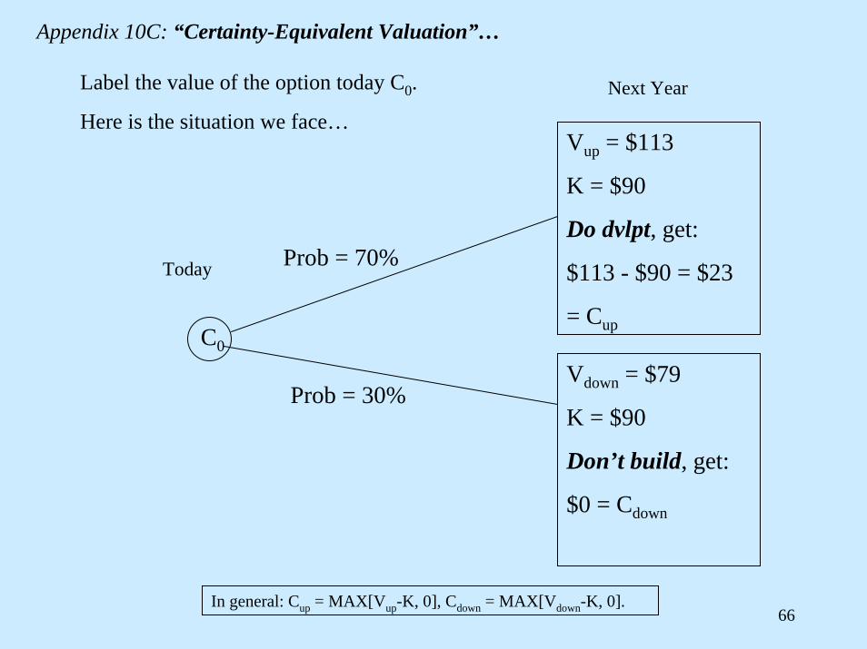
66
Vup = $113
K = $90
Do dvlpt, get:
$113 - $90 = $23
= Cup
Vdown = $79
K = $90
Don’t build, get:
$0 = Cdown
Prob = 70%
Prob = 30%
C0
Label the value of the option today C0.
Here is the situation we face…
Today
Next Year
In general: Cup = MAX[Vup-K, 0], Cdown = MAX[Vdown-K, 0].
Appendix 10C: “Certainty-Equivalent Valuation”…
67
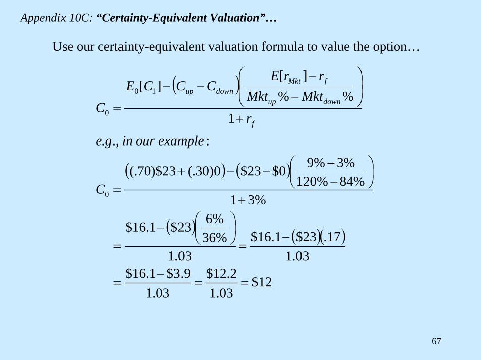
Use our certainty-equivalent valuation formula to value the option…
( )
( ) ( )
( ) ( )( )
12$03.1
2.12$03.1
9.3$1.16$03.1
17.23$1.16$03.1
%36%623$1.16$
%31%84%120
%3%90$23$0)30(.23)$70(.
:.,.
1%%
][][
0
10
0
==−
=
−=
⎟⎠⎞
⎜⎝⎛−
=
+
⎟⎠⎞
⎜⎝⎛
−−
−−+=
+
⎟⎟⎠
⎞⎜⎜⎝
⎛
−−
−−
=
C
exampleouringe
rMktMkt
rrECCCE
Cf
downup
fMktdownup
Appendix 10C: “Certainty-Equivalent Valuation”…
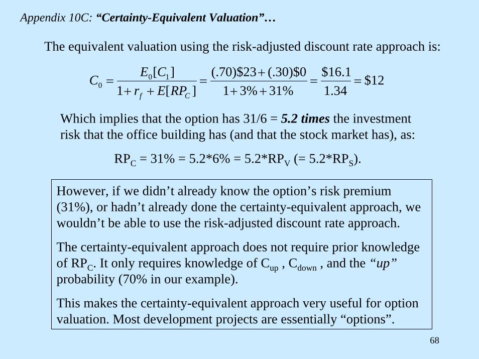
68
12$34.1
1.16$%31%31
0)$30(.23)$70(.][1
][ 100 ==
+++
=++
=Cf RPEr
CEC
The equivalent valuation using the risk-adjusted discount rate approach is:
Which implies that the option has 31/6 = 5.2 times the investment risk that the office building has (and that the stock market has), as:
RPC = 31% = 5.2*6% = 5.2*RPV (= 5.2*RPS).
However, if we didn’t already know the option’s risk premium (31%), or hadn’t already done the certainty-equivalent approach, we wouldn’t be able to use the risk-adjusted discount rate approach.
The certainty-equivalent approach does not require prior knowledge of RPC. It only requires knowledge of Cup , Cdown , and the “up”probability (70% in our example).
This makes the certainty-equivalent approach very useful for option valuation. Most development projects are essentially “options”.
Appendix 10C: “Certainty-Equivalent Valuation”…
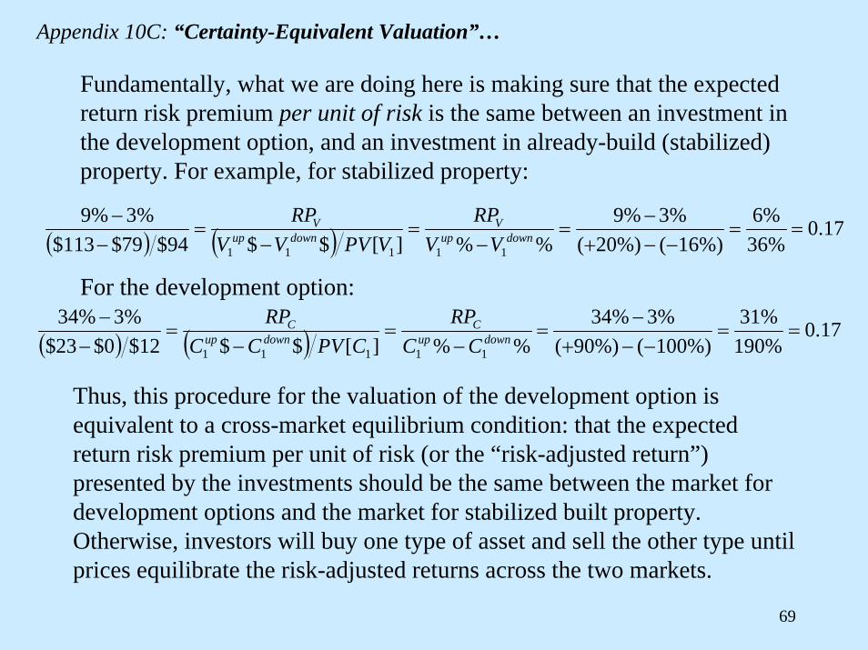
69
( ) ( ) 17.0%36%6
%)16(%)20(%3%9
%%][$$94$79$113$%3%9
11111
==−−+
−=
−=
−=
−−
downupV
downupV
VVRP
VPVVVRP
( )
Fundamentally, what we are doing here is making sure that the expected return risk premium per unit of risk is the same between an investment in the development option, and an investment in already-build (stabilized) property. For example, for stabilized property:
Appendix 10C: “Certainty-Equivalent Valuation”…
( ) 17.0%190%31
%)100(%)90(%3%34
%%][$$12$0$23$%3%34
11111
==−−+
−=
−=
−=
−−
downupC
downupC
CCRP
CPVCCRP
For the development option:
Thus, this procedure for the valuation of the development option is equivalent to a cross-market equilibrium condition: that the expected return risk premium per unit of risk (or the “risk-adjusted return”) presented by the investments should be the same between the market for development options and the market for stabilized built property. Otherwise, investors will buy one type of asset and sell the other type until prices equilibrate the risk-adjusted returns across the two markets.