Chapter 10 Matching Markets - Cornell CS Top-Level

Chapter 10

Matching Markets

From the book Networks, Crowds, and Markets: Reasoning about a Highly Connected World.By David Easley and Jon Kleinberg. Cambridge University Press, 2010.Complete preprint on-line at http://www.cs.cornell.edu/home/kleinber/networks-book/

We have now seen a number of ways of thinking both about network structure and

about the behavior of agents as they interact with each other. A few of our examples have

brought these together directly — such as the issue of traffic in a network, including Braess’s

Paradox — and in the next few chapters we explore this convergence of network structure

and strategic interaction more fully, and in a range of different settings.

First, we think about markets as a prime example of network-structured interaction

between many agents. When we consider markets creating opportunities for interaction

among buyers and sellers, there is an implicit network encoding the access between these

buyers and sellers. In fact, there are a number of ways of using networks to model interactions

among market participants, and we will discuss several of these models. Later, in Chapter 12

on network exchange theory, we will discuss how market-style interactions become a metaphor

for the broad notion of social exchange, in which the social dynamics within a group can be

modeled by the power imbalances of the interactions within the group’s social network.

10.1 Bipartite Graphs and Perfect Matchings

Matching markets form the first class of models we consider, as the focus of the current

chapter. Matching markets have a long history of study in economics, operations research,

and other areas because they embody, in a very clean and stylized way, a number of basic

principles: the way in which people may have different preferences for different kinds of

goods, the way in which prices can decentralize the allocation of goods to people, and the

way in which such prices can in fact lead to allocations that are socially optimal.

We will introduce these various ingredients gradually, by progressing through a succession

of increasingly rich models. We begin with a setting in which goods will be allocated to people

Draft version: June 10, 2010

277

278 CHAPTER 10. MATCHING MARKETS

Room1

Room2

Room3

Room4

Room5

Vikram

Wendy

Xin

Yoram

Zoe

(a) Bipartite Graph

Room1

Room2

Room3

Room4

Room5

Vikram

Wendy

Xin

Yoram

Zoe

(b) A Perfect Matching

Figure 10.1: (a) An example of a bipartite graph. (b) A perfect matching in this graph,indicated via the dark edges.

based on preferences, and these preferences will be expressed in network form, but there is

no explicit buying, selling, or price-setting. This first setting will also be a crucial component

of the more complex ones that follow.

Bipartite Graphs. The model we start with is called the bipartite matching problem, and

we can motivate it via the following scenario. Suppose that the administrators of a college

dormitory are assigning rooms to returning students for a new academic year; each room

is designed for a single student, and each student is asked to list several acceptable options

for the room they’d like to get. Students can have different preferences over rooms; some

people might want larger rooms, quieter rooms, sunnier rooms, and so forth — and so the

lists provided by the students may overlap in complex ways.

We can model the lists provided by the students using a graph, as follows. There is a

node for each student, a node for each room, and an edge connecting a student to a room if

the student has listed the room as an acceptable option. Figure 10.1(a) shows an example

with five students and five rooms (indicating, for instance, that the student named Vikram

has listed each of Rooms 1, 2, and 3 as acceptable options, while the student named Wendy

only listed Room 1).

This type of graph is bipartite, an important property that we saw earlier, in a different

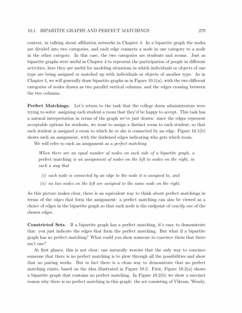
10.1. BIPARTITE GRAPHS AND PERFECT MATCHINGS 279

context, in talking about affiliation networks in Chapter 4. In a bipartite graph the nodes

are divided into two categories, and each edge connects a node in one category to a node

in the other category. In this case, the two categories are students and rooms. Just as

bipartite graphs were useful in Chapter 4 to represent the participation of people in different

activities, here they are useful for modeling situations in which individuals or objects of one

type are being assigned or matched up with individuals or objects of another type. As in

Chapter 4, we will generally draw bipartite graphs as in Figure 10.1(a), with the two different

categories of nodes drawn as two parallel vertical columns, and the edges crossing between

the two columns.

Perfect Matchings. Let’s return to the task that the college dorm administrators were

trying to solve: assigning each student a room that they’d be happy to accept. This task has

a natural interpretation in terms of the graph we’ve just drawn: since the edges represent

acceptable options for students, we want to assign a distinct room to each student, so that

each student is assigned a room to which he or she is connected by an edge. Figure 10.1(b)

shows such an assignment, with the darkened edges indicating who gets which room.

We will refer to such an assignment as a perfect matching:

When there are an equal number of nodes on each side of a bipartite graph, a

perfect matching is an assignment of nodes on the left to nodes on the right, in

such a way that

(i) each node is connected by an edge to the node it is assigned to, and

(ii) no two nodes on the left are assigned to the same node on the right.

As this picture makes clear, there is an equivalent way to think about perfect matchings in

terms of the edges that form the assignment: a perfect matching can also be viewed as a

choice of edges in the bipartite graph so that each node is the endpoint of exactly one of the

chosen edges.

Constricted Sets. If a bipartite graph has a perfect matching, it’s easy to demonstrate

this: you just indicate the edges that form the perfect matching. But what if a bipartite

graph has no perfect matching? What could you show someone to convince them that there

isn’t one?

At first glance, this is not clear; one naturally worries that the only way to convince

someone that there is no perfect matching is to plow through all the possibilities and show

that no pairing works. But in fact there is a clean way to demonstrate that no perfect

matching exists, based on the idea illustrated in Figure 10.2. First, Figure 10.2(a) shows

a bipartite graph that contains no perfect matching. In Figure 10.2(b) we show a succinct

reason why there is no perfect matching in this graph: the set consisting of Vikram, Wendy,


Room1

Room2

Room3

Room4

Room5

Vikram

Wendy

Xin

Yoram

Zoe

(a) Bipartite graph with no perfectmatching

Room1

Room2

Room3

Room4

Room5

Vikram

Wendy

Xin

Yoram

Zoe

(b) A constricted set demonstratingthere is no perfect matching

Figure 10.2: (a) A bipartite graph with no perfect matching. (b) A constricted set demon-strating there is no perfect matching.

and Xin, taken together, has collectively provided only two options for rooms that would

be acceptable to any of them. With three people and only two acceptable rooms, there is

clearly no way to construct a perfect matching — one of these three people would have to

get an option they didn’t want in any assignment of rooms.

We call the set of three students in this example a constricted set, since their edges to

the other side of the bipartite graph “constrict” the formation of a perfect matching. This

example points to a general phenomenon, which we can make precise by defining in general

what it means for a set to be constricted, as follows. First, for any set of nodes S on the

right-hand side of a bipartite graph, we say that a node on the left-hand side is a neighbor

of S if it has an edge to some node in S. We define the neighbor set of S, denoted N(S), to

be the collection of all neighbors of S. Finally, we say that a set S on the right-hand side is

constricted if S is strictly larger than N(S) — that is, S contains strictly more nodes than

N(S) does.

Any time there’s a constricted set S in a bipartite graph, it immediately shows that there

can be no perfect matching: each node in S would have to be matched to a different node

in N(S), but there are more nodes in S than there are in N(S), so this is not possible.

10.1. BIPARTITE GRAPHS AND PERFECT MATCHINGS 281

Room1

Room2

Room3

Xin

Yoram

Zoe

12, 2, 4

8, 7, 6

7, 5, 2

Valuations

(a) A set of valuations

Room1

Room2

Room3

Xin

Yoram

Zoe

12, 2, 4

8, 7, 6

7, 5, 2

Valuations

(b) An optimal assignment

Figure 10.3: (a) A set of valuations. Each person’s valuations for the objects appears as alist next to them. (b) An optimal assignment with respect to these valuations.

So it’s fairly easy to see that constricted sets form one kind of obstacle to the presence of

perfect matchings. What’s also true, though far from obvious, is that constricted sets are in

fact the only kind of obstacle. This is the crux of the following fact, known as the Matching

Theorem.

Matching Theorem: If a bipartite graph (with equal numbers of nodes on the left

and right) has no perfect matching, then it must contain a constricted set.

The Matching Theorem was independently discovered by Denes Konig in 1931 and Phillip

Hall in 1935 [280]. Without the theorem, one might have imagined that a bipartite graph

could fail to have a perfect matching for all sorts of reasons, some of them perhaps even too

complicated to explain; but what the theorem says is that the simple notion of a constricted

set is in fact the only obstacle to having a perfect matching. For our purposes in this chapter,

we will only need to use the fact that the Matching Theorem is true, without having to go

into the details of its proof. However, its proof is elegant as well, and we describe a proof of

the theorem in Section 10.6 at the end of this chapter.

One way to think about the Matching Theorem, using our example of students and

rooms, is as follows. After the students submit their lists of acceptable rooms, it’s easy for

the dormitory administrators to explain to the students what happened, regardless of the

outcome. Either they can announce the perfect matching giving the assignment of students

to rooms, or they can explain that no assignment is possible by indicating a set of students

who collectively gave too small a set of acceptable options. This latter case is a constricted

set.


Room1

Room2

Room3

Xin

Yoram

Zoe

(a) A bipartite graph

Room1

Room2

Room3

Xin

Yoram

Zoe

1, 1, 0

1, 0, 0

0, 1, 1

(b) A set of valuations encoding the search for a perfectmatching

Figure 10.4: (a) A bipartite graph in which we want to search for a perfect matching. (b) Acorresponding set of valuations for the same nodes so that finding the optimal assignmentlets us determine whether there is a perfect matching in the original graph.

10.2 Valuations and Optimal Assignments

The problem of bipartite matching from the previous section illustrates some aspects of a

market in a very simple form: individuals express preferences in the form of acceptable op-

tions; a perfect matching then solves the problem of allocating objects to individuals accord-

ing to these preferences; and if there is no perfect matching, it is because of a “constriction”

in the system that blocks it.

We now want to extend this model to introduce some additional features. First, rather

than expressing preferences simply as binary “acceptable-or-not” choices, we allow each

individual to express how much they’d like each object, in numerical form. In our example

of students and dorm rooms from Section 10.1, suppose that rather than specifying a list

of acceptable rooms, each student provides a numerical score for each room, indicating how

happy they’d be with it. We will refer to these numbers as the students’ valuations for the

respective rooms. Figure 10.3(a) shows an example of this with three students and three

rooms; for instance, Xin’s valuations for Rooms 1, 2, and 3 are 12, 2, and 4 respectively

(while Yoram’s valuations for Rooms 1, 2, and 3 are 8, 7, and 6 respectively). Notice that

students may disagree on which rooms are better, and by how much.

We can define valuations whenever we have a collection of individuals evaluating a col-

lection of objects. And using these valuations, we can evaluate the quality of an assignment

of objects to individuals, as follows: it is the sum of each individual’s valuation for what

10.2. VALUATIONS AND OPTIMAL ASSIGNMENTS 283

they get.1 Thus, for example, the quality of the assignment illustrated in Figure 10.3(b) is

12 + 6 + 5 = 23.

If the dorm administrators had accurate data on each student’s valuations for each room,

then a reasonable way to assign rooms to students would be to choose the assignment of

maximum possible quality. We will refer to this as the optimal assignment, since it maximizes

the total happiness of everyone for what they get. You can check that the assignment in

Figure 10.3(b) is in fact the optimal assignment for this set of valuations. Of course, while

the optimal assignment maximizes total happiness, it does not necessarily give everyone their

favorite item; for example, in Figure 10.3(b), all the students think Room 1 is the best, but

it can only go to one of them.

In a very concrete sense, the problem of finding an optimal assignment also forms a

natural generalization of the bipartite matching problem from Section 10.1. Specifically,

it contains the bipartite matching problem as a special case. Here is why. Suppose, as in

Section 10.1, that there are an equal number of students and rooms, and each student simply

submits a list of acceptable rooms without providing a numerical valuation; this gives us a

bipartite graph as in Figure 10.4(a). We would like to know if this bipartite graph contains

a perfect matching, and we can express precisely this question in the language of valuations

and optimal assignments as follows. We give each student a valuation of 1 for each room

they included on their acceptable list, and a valuation of 0 for each room they omitted from

their list. Applying this translation to the graph in Figure 10.4(a), for example, we get the

valuations shown in Figure 10.4(b). Now, there is a perfect matching precisely when we can

find an assignment that gives each student a room that he or she values at 1 rather than 0

— that is, precisely when the optimal assignment has a total valuation equal to the number

of students. This simple translation shows how the problem of bipartite matching is implicit

in the broader problem of finding an optimal assignment.

While the definition of an optimal assignment is quite natural and general, it is far

from obvious whether there is a comparably natural way to find or characterize the optimal

assignment for a given set of valuations. This is in fact a bit subtle; we will describe a way

to determine an optimal assignment, in the context of a broader market interpretation of

this problem, in the two next sections.

1Of course, this notion of the quality of an assignment is appropriate only if adding individual’s valuationsmakes sense. We can interpret individual valuations here as the maximum amount the individuals are willingto pay for items, so the sum of their valuations for the items they are assigned is just the maximum amountthe group would be willing to pay in total for the assignment. The issue of adding individuals’ payoffs wasalso discussed in Chapter 6, where we defined social optimality using the sum of payoffs in a game.


10.3 Prices and the Market-Clearing Property

Thus far, we have been using the metaphor of a central “administrator” who determines

a perfect matching, or an optimal assignment, by collecting data from everyone and then

performing a centralized computation. And while there are clearly instances of market-like

activity that function this way (such as our example of students and dorm rooms), a more

standard picture of a market involves much less central coordination, with individuals making

decisions based on prices and their own valuations.

Capturing this latter idea brings us to the crucial step in our formulation of matching

markets: understanding the way in which prices can serve to decentralize the market. We

will see that if we replace the role of the central administrator by a particular scheme for

pricing items, then allowing individuals to follow their own self-interest based on valuations

and prices can still produce optimal assignments.

To describe this, let’s change the housing metaphor slightly, from students and dorm

rooms to one where the role of prices is more natural. Suppose that we have a collection

of sellers, each with a house for sale, and an equal-sized collection of buyers, each of whom

wants a house. By analogy with the previous section, each buyer has a valuation for each

house, and as before, two different buyers may have very different valuations for the same

houses. The valuation that a buyer j has for the house held by seller i will be denoted vij,

with the subscripts i and j indicating that the valuation depends on both the identity of

the seller i and the buyer j. We also assume that each valuation is a non-negative whole

number (0, 1, 2, . . .). We assume that sellers have a valuation of 0 for each house; they care

only about receiving payment from buyers, which we define next.2

Prices and Payoffs. Suppose that each seller i puts his house up for sale, offering to sell

it for a price pi ≥ 0. If a buyer j buys the house from seller i at this price, we will say that

the buyer’s payoff is her valuation for this house, minus the amount of money she had to pay:

vij − pi. So given a set of prices, if buyer j wants to maximize her payoff, she will buy from

the seller i for which this quantity vij − pi is maximized — with the following caveats. First,

if this quantity is maximized in a tie between several sellers, then the buyer can maximize

her payoff by choosing any one of them. Second, if her payoff vij − pi is negative for every

choice of seller i, then the buyer would prefer not to buy any house: we assume she can

obtain a payoff of 0 by simply not transacting.

We will call the seller or sellers that maximize the payoff for buyer j the preferred sellers

2Our assumption that sellers all have valuations of 0 for their houses is done for the sake of simplicity; ifwe wanted, we could directly adapt the arguments here to the case in which “zero” is really some minimumbase level, and all other valuations and prices represent amounts above this base level. It is also not hard toadapt our analysis to the case in which sellers each might have different valuations for their houses. Sincenone of these more general models add much to the underlying set of ideas, we will stick with the simpleassumption that sellers have valuations of 0 for houses.

10.3. PRICES AND THE MARKET-CLEARING PROPERTY 285

a

b

c

x

y

z

12, 4, 2

8, 7, 6

7, 5, 2

Sellers Buyers Valuations

(a) Buyer Valuations

a

b

c

x

y

z

12, 4, 2

8, 7, 6

7, 5, 2

5

2

0

Prices Sellers Buyers Valuations

(b) Market-Clearing Prices

a

b

c

x

y

z

12, 4, 2

8, 7, 6

7, 5, 2

2

1

0


(c) Prices that Don’t Clear the Market

a

b

c

x

y

z

12, 4, 2

8, 7, 6

7, 5, 2

3

1

0


(d) Market-Clearing Prices (Tie-Breaking Required)

Figure 10.5: (a) Three sellers (a, b, and c) and three buyers (x, y, and z). For each buyer node, thevaluations for the houses of the respective sellers appear in a list next to the node. (b) Each buyer creates alink to her preferred seller. The resulting set of edges is the preferred-seller graph for this set of prices. (c)The preferred-seller graph for prices 2, 1, 0. (d) The preferred-seller graph for prices 3, 1, 0.

of buyer j, provided the payoff from these sellers is not negative. We say that buyer j has

no preferred seller if the payoffs vij − pi are negative for all choices of i.

In Figures 10.5(b)-10.5(d), we show the results of three different sets of prices for the

same set of buyer valuations. Note how the sets of preferred sellers for each buyer change

depending on what the prices are. So for example, in Figure 10.5(b), buyer x would receive a

payoff of 12−5 = 7 if she buys from a, a payoff of 4−2 = 2 if she buys from b, and 2−0 = 2

if she buys from c. This is why a is her unique preferred seller. We can similarly determine

the payoffs for buyers y (3, 5, and 6) and z (2, 3, and 2) for transacting with sellers a, b, and

c respectively.


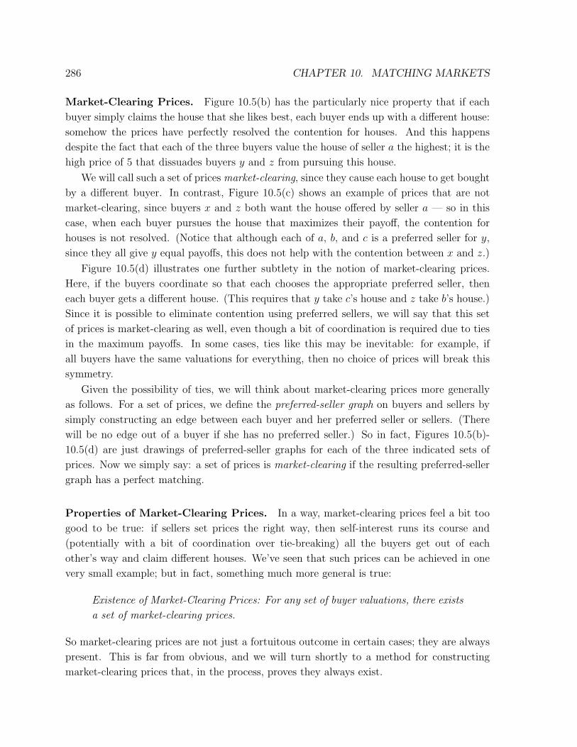
Market-Clearing Prices. Figure 10.5(b) has the particularly nice property that if each

buyer simply claims the house that she likes best, each buyer ends up with a different house:

somehow the prices have perfectly resolved the contention for houses. And this happens

despite the fact that each of the three buyers value the house of seller a the highest; it is the

high price of 5 that dissuades buyers y and z from pursuing this house.

We will call such a set of prices market-clearing, since they cause each house to get bought

by a different buyer. In contrast, Figure 10.5(c) shows an example of prices that are not

market-clearing, since buyers x and z both want the house offered by seller a — so in this

case, when each buyer pursues the house that maximizes their payoff, the contention for

houses is not resolved. (Notice that although each of a, b, and c is a preferred seller for y,

since they all give y equal payoffs, this does not help with the contention between x and z.)

Figure 10.5(d) illustrates one further subtlety in the notion of market-clearing prices.

Here, if the buyers coordinate so that each chooses the appropriate preferred seller, then

each buyer gets a different house. (This requires that y take c’s house and z take b’s house.)

Since it is possible to eliminate contention using preferred sellers, we will say that this set

of prices is market-clearing as well, even though a bit of coordination is required due to ties

in the maximum payoffs. In some cases, ties like this may be inevitable: for example, if

all buyers have the same valuations for everything, then no choice of prices will break this

symmetry.

Given the possibility of ties, we will think about market-clearing prices more generally

as follows. For a set of prices, we define the preferred-seller graph on buyers and sellers by

simply constructing an edge between each buyer and her preferred seller or sellers. (There

will be no edge out of a buyer if she has no preferred seller.) So in fact, Figures 10.5(b)-

10.5(d) are just drawings of preferred-seller graphs for each of the three indicated sets of

prices. Now we simply say: a set of prices is market-clearing if the resulting preferred-seller

graph has a perfect matching.

Properties of Market-Clearing Prices. In a way, market-clearing prices feel a bit too

good to be true: if sellers set prices the right way, then self-interest runs its course and

(potentially with a bit of coordination over tie-breaking) all the buyers get out of each

other’s way and claim different houses. We’ve seen that such prices can be achieved in one

very small example; but in fact, something much more general is true:

Existence of Market-Clearing Prices: For any set of buyer valuations, there exists

a set of market-clearing prices.

So market-clearing prices are not just a fortuitous outcome in certain cases; they are always

present. This is far from obvious, and we will turn shortly to a method for constructing

market-clearing prices that, in the process, proves they always exist.

10.3. PRICES AND THE MARKET-CLEARING PROPERTY 287

Before doing this, we consider another natural question: the relationship between market-

clearing prices and social welfare. Just because market-clearing prices resolve the contention

among buyers, causing them to get different houses, does this mean that the total valuation

of the resulting assignment will be good? In fact, there is something very strong that can

be said here as well: market-clearing prices (for this buyer-seller matching problem) always

provide socially optimal outcomes:

Optimality of Market-Clearing Prices: For any set of market-clearing prices, a

perfect matching in the resulting preferred-seller graph has the maximum total

valuation of any assignment of sellers to buyers.

Compared with the previous claim on the existence of market-clearing prices, this fact about

optimality can be justified by a much shorter, if somewhat subtle, argument.

The argument is as follows. Consider a set of market-clearing prices, and let M be

a perfect matching in the preferred-seller graph. Now, consider the total payoff of this

matching, defined simply as the sum of each buyer’s payoff for what she gets. Since each

buyer is grabbing a house that maximizes her payoff individually, M has the maximum total

payoff of any assignment of houses to buyers. Now how does total payoff relate to total

valuation, which is what we’re hoping that M maximizes? If buyer j chooses house i, then

her valuation is vij and her payoff is vij − pi. Thus, the total payoff to all buyers is simply

the total valuation, minus the sum of all prices:

Total Payoff of M = Total Valuation of M − Sum of all prices.

But the sum of all prices is something that doesn’t depend on which matching we choose

(it’s just the sum of everything the sellers are asking for, regardless of how they get paired up

with buyers). So a matching M that maximizes the total payoff is also one that maximizes

the total valuation. This completes the argument.

There is another important way of thinking about the optimality of market-clearing

prices, which turns out to be essentially equivalent to the formulation we’ve just described.

Suppose that instead of thinking about the total valuation of the matching, we think about

the total of the payoffs received by all participants in the market — both the sellers and

the buyers. For a buyer, her payoff is defined as above: it is her valuation for the house she

gets minus the price she pays. A seller’s payoff is simply the amount of money he receives in

payment for his house. Therefore, in any matching, the total of the payoffs to all the sellers

is simply equal to the sum of the prices (since they all get paid, and it doesn’t matter which

buyer pays which seller). Above, we just argued that the total of the payoffs to all the buyers

is equal to the total valuation of the matching M , minus the sum of all prices. Therefore,

the total of the payoffs to all participants — both the sellers and the buyers — is exactly

equal to the total valuation of the matching M ; the point is that the prices detract from


the total buyer payoff by exactly the amount that they contribute to the total seller payoff,

and hence the sum of the prices cancels out completely from this calculation. Therefore,

to maximize the total payoffs to all participants, we want prices and a matching that lead

to the maximum total valuation, and this is achieved by using market-clearing prices and a

perfect matching in the resulting preferred-seller graph. We can summarize this as follows.

Optimality of Market-Clearing Prices (equivalent version): A set of market-

clearing prices, and a perfect matching in the resulting preferred-seller graph,

produces the maximum possible sum of payoffs to all sellers and buyers.

10.4 Constructing a Set of Market-Clearing Prices

Now let’s turn to the harder challenge: understanding why market-clearing prices must

always exist. We’re going to do this by taking an arbitrary set of buyer valuations, and

describing a procedure that arrives at market-clearing prices. The procedure will in fact

be a kind of auction — not a single-item auction of the type we discussed in Chapter 9,

but a more general kind taking into account the fact that there are multiple things being

auctioned, and multiple buyers with different valuations. This particular auction procedure

was described by the economists Demange, Gale, and Sotomayor in 1986 [129], but it’s

actually equivalent to a construction of market-clearing prices discovered by the Hungarian

mathematician Egervary seventy years earlier, in 1916 [280].

Here’s how the auction works. Initially all sellers set their prices to 0. Buyers react by

choosing their preferred seller(s), and we look at the resulting preferred-seller graph. If this

graph has a perfect matching we’re done. Otherwise — and this is the key point — there is

a constricted set of buyers S. Consider the set of neighbors N(S), which is a set of sellers.

The buyers in S only want what the sellers in N(S) have to sell, but there are fewer sellers

in N(S) than there are buyers in S. So the sellers in N(S) are in “high demand” — too

many buyers are interested in them. They respond by each raising their prices by one unit,

and the auction then continues.

There’s one more ingredient, which is a reduction operation on the prices. It will be

useful to have our prices scaled so that the smallest one is 0. Thus, if we ever reach a point

where all prices are strictly greater than 0 — suppose the smallest price has value p > 0 —

then we reduce the prices by subtracting p from each one. This drops the lowest price to 0,

and shifts all other prices by the same relative amount.

A general round of the auction looks like what we’ve just described.

(i) At the start of each round, there is a current set of prices, with the smallest

one equal to 0.

(ii) We construct the preferred-seller graph and check whether there is a perfect

matching.

10.4. CONSTRUCTING A SET OF MARKET-CLEARING PRICES 289

(iii) If there is, we’re done: the current prices are market-clearing.

(iv) If not, we find a constricted set of buyers S and their neighbors N(S).

(v) Each seller in N(S) (simultaneously) raises his price by one unit.

(vi) If necessary, we reduce the prices — the same amount is subtracted from

each price so that the smallest price becomes zero.

(vii) We now begin the next round of the auction, using these new prices.

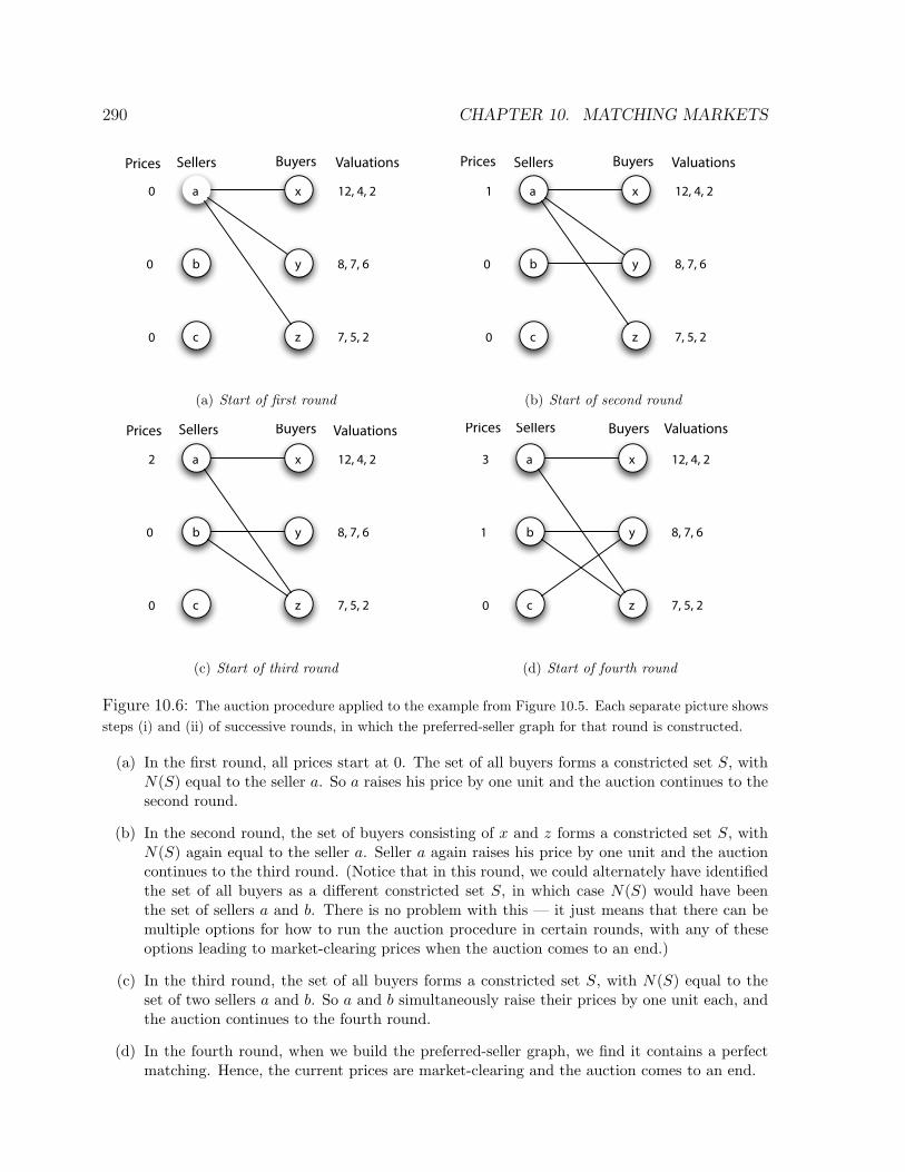
The full-page Figure 10.6 shows what happens when we apply the auction procedure to the

example from Figure 10.5.

The example in Figure 10.6 illustrates two aspects of this auction that should be empha-

sized. First, in any round where the set of “over-demanded” sellers N(S) consists of more

than one individual, all the sellers in this set raise their prices simultaneously. For example,

in the third round in Figure 10.6, the set N(S) consists of both a and b, and so they both

raise their prices so as to produce the prices used for the start of the fourth round. Second,

while the auction procedure shown in Figure 10.6 produces the market-clearing prices shown

in Figure 10.5(d), we know from Figure 10.5(b) that there can be other market-clearing

prices for the same set of buyer valuations.

Showing that the Auction Must Come to an End. Here is a key property of the

auction procedure we’ve defined: the only way it can come to end is if it reaches a set of

market-clearing prices; otherwise, the rounds continue. So if we can show that the auction

must come to an end for any set of buyer valuations — i.e. that the rounds cannot go on

forever — then we’ve shown that market-clearing prices always exist.

It’s not immediately clear, however, why the auction must always come to an end. Con-

sider, for example, the sequence of steps the auction follows in Figure 10.6: prices change,

different constricted sets form at different points in time, and eventually the auction stops

with a set of market-clearing prices. But why should this happen in general? Why couldn’t

there be a set of valuations that cause the prices to constantly shift around so that some set

of buyers is always constricted, and the auction never stops?

In fact, the prices can’t shift forever without stopping; the auction must always come to

an end. The way we’re going to show this is by identifying a precise sense in which a certain

kind of “potential energy” is draining out of the auction as it runs; since the auction starts

with only a bounded supply of this potential energy at the beginning, it must eventually run

out.

Here is how we define this notion of potential energy precisely. For any current set of

prices, define the potential of a buyer to be the maximum payoff she can currently get from

any seller. This is the buyer’s potential payoff; the buyer will actually get this payoff if the

current prices are market-clearing prices. We also define the potential of a seller to be the


a

b

c

x

y

z

12, 4, 2

8, 7, 6

7, 5, 2

0

0

0


(a) Start of first round

a

b

c

x

y

z

12, 4, 2

8, 7, 6

7, 5, 2

1

0

0


(b) Start of second round

a

b

c

x

y

z

12, 4, 2

8, 7, 6

7, 5, 2

2

0

0


(c) Start of third round

a

b

c

x

y

z

12, 4, 2

8, 7, 6

7, 5, 2

3

1

0


(d) Start of fourth round

Figure 10.6: The auction procedure applied to the example from Figure 10.5. Each separate picture showssteps (i) and (ii) of successive rounds, in which the preferred-seller graph for that round is constructed.

(a) In the first round, all prices start at 0. The set of all buyers forms a constricted set S, withN(S) equal to the seller a. So a raises his price by one unit and the auction continues to thesecond round.

(b) In the second round, the set of buyers consisting of x and z forms a constricted set S, withN(S) again equal to the seller a. Seller a again raises his price by one unit and the auctioncontinues to the third round. (Notice that in this round, we could alternately have identifiedthe set of all buyers as a different constricted set S, in which case N(S) would have beenthe set of sellers a and b. There is no problem with this — it just means that there can bemultiple options for how to run the auction procedure in certain rounds, with any of theseoptions leading to market-clearing prices when the auction comes to an end.)

(c) In the third round, the set of all buyers forms a constricted set S, with N(S) equal to theset of two sellers a and b. So a and b simultaneously raise their prices by one unit each, andthe auction continues to the fourth round.

(d) In the fourth round, when we build the preferred-seller graph, we find it contains a perfectmatching. Hence, the current prices are market-clearing and the auction comes to an end.

10.5. HOW DOES THIS RELATE TO SINGLE-ITEM AUCTIONS? 291

current price he is charging. This is the seller’s potential payoff; the seller will actually get

this payoff if the current prices are market-clearing prices. Finally, we define the potential

energy of the auction to be the sum of the potential of all participants, both buyers and

sellers.

How does the potential energy of the auction behave as we run it? It begins with all

sellers having potential 0, and each buyer having a potential equal to her maximum valuation

for any house — so the potential energy of the auction at the start is some whole number

P0 ≥ 0. Also, notice that at the start of each round of the auction, everyone has potential

at least 0. The sellers always have potential at least 0 since the prices are always at least 0.

Because of the price-reduction step in every round, the lowest price is always 0, and therefore

each buyer is always doing at least as well as the option of buying a 0-cost item, which gives

a payoff of at least 0. (This also means that each buyer has at least one preferred seller at

the start of each round.) Finally, since the potentials of the sellers and buyers are all at least

0 at the start of each round, so is the potential energy of the auction.

Now, the potential only changes when the prices change, and this only happens in steps

(v) and (vi). Notice that the reduction of prices, as defined above, does not change the

potential energy of the auction: if we subtract p from each price, then the potential of each

seller drops by p, but the potential of each buyer goes up by p — it all cancels out. Finally,

what happens to the potential energy of the auction in step (v), when the sellers in N(S)

all raise their prices by one unit? Each of these sellers’ potentials goes up by one unit. But

the potential of each buyer in S goes down by one unit, since all their preferred houses just

got more expensive. Since S has strictly more nodes than N(S) does, this means that the

potential energy of the auction goes down by at least one unit more than it goes up, so it

strictly decreases by at least one unit.

So what we’ve shown is that in each step that the auction runs, the potential energy of

the auction decreases by at least one unit. It starts at some fixed value P0, and it can’t drop

below 0, so the auction must come to an end within P0 steps — and when it comes to an

end, we have our market-clearing prices.

10.5 How Does this Relate to Single-Item Auctions?

We talked in Chapter 9 about single-item auctions, and we’ve now seen a more complex

type of auction based on bipartite graphs. It makes sense to ask how these different kinds

of auctions relate to each other. In fact, there is a very natural way to view the single-item

auction — both the outcome and the procedure itself — as a special case of the bipartite

graph auction we’ve just defined. We can do this as follows.

Suppose we have a set of n buyers and a single seller auctioning an item; let buyer j

have valuation vj for the item. To map this to our model based on perfect matchings, we


a

b

c

x

y

z

3, 0, 0

2, 0, 0

1, 0, 0

0

0

0


(a) Start of the Auction

a

b

c

x

y

z

3, 0, 0

2, 0, 0

1, 0, 0

2

0

0


(b) End of the Auction

Figure 10.7: A single-item auction can be represented by the bipartite graph model: theitem is represented by one seller node, and then there are additional seller nodes for whichall buyers have 0 valuation. (a) The start of the bipartite graph auction. (b) The end of thebipartite graph auction, when buyer x gets the item at the valuation of buyer y.

need an equal number of buyers and sellers, but this is easily dealt with: we create n − 1

“fake” additional sellers (who conceptually represent n − 1 different ways to fail to acquire

the item), and we give buyer j a valuation of 0 for the item offered by each of these fake

sellers. With the real seller labeled 1, this means we have v1j = vj, the valuation of buyer j

for the real item; and vij = 0 for larger values of i.

Now we have a genuine instance of our bipartite graph model: from a perfect matching

of buyers to sellers, we can see which buyer ends up paired with the real seller (this is the

buyer who gets the item), and from a set of market-clearing prices, we will see what the real

item sells for.

Moreover, the price-raising procedure to produce market-clearing prices — based on

finding constricted sets — has a natural meaning here as well. The execution of the procedure

on a simple example is shown in Figure 10.7. Initially, all buyers will identify the real seller

as their preferred seller (assuming that they all have positive valuations for the item). The

first constricted set S we find is the set of all buyers, and N(S) is just the single real seller.

Thus, the seller raises his price by one unit. This continues as long as at least two buyers

have the real seller as their unique preferred seller: they form a constricted set S with N(S)

equal to the real seller, and this seller raises his price by a unit. The prices of the fake items

remain fixed at 0 throughout the auction. Finally, when all but one buyer has identified other

sellers as preferred sellers, the graph has a perfect matching. This happens at precisely the

moment that the buyer with the second-highest valuation drops out — in other words, the

buyer with the highest valuation gets the item, and pays the second-highest valuation. So

the bipartite graph procedure precisely implements an ascending bid (English) auction.

10.6. ADVANCED MATERIAL: A PROOF OF THE MATCHING THEOREM 293

10.6 Advanced Material: A Proof of the MatchingTheorem

The discussion in this chapter provides a complete proof that market-clearing prices exist,

omitting the details in only one place: we deferred the proof of the Matching Theorem

in Section 10.1, since it was enough for our purposes to use it in a “black-box” fashion.

However, the standard proof of the Matching Theorem in fact provides important insights

into the structure of bipartite graphs, and so we present it here.

Recall that the statement is the following.

Claim: If a bipartite graph (with equal numbers of nodes on the left and right)

has no perfect matching, then it must contain a constricted set.

The tricky part of proving this is to come up with some means of identifying a constricted

set in a bipartite graph, knowing only that it contains no perfect matching. Our general

plan for doing this will be as follows. We will take a bipartite graph, with equal numbers of

nodes on the left and right but no perfect matching, and consider a matching that includes

as many nodes as possible — we will call this a maximum matching. We then try to enlarge

it, by searching for a way to include one more node from each side in the matching. This

will fail (since the matching is already as large as possible for the given graph), and we show

that when this search for a larger matching fails, it produces a constricted set.

Naturally, there is a lot that needs to be fleshed out in this strategy, and the first step is

to consider how one goes about “enlarging” a matching in a bipartite graph. This will turn

out to be the key issue in the whole proof.

Alternating and Augmenting Paths. With this in mind, let’s forget about constricted

sets for a little while and simply think about matchings and how they can be enlarged. As a

first example, consider the bipartite graph in Figure 10.8(a), with a matching indicated using

bold edges. (We’ll say that the matching edges are the edges used in a given matching, and

the non-matching edges are the other, unused ones.) The matching shown in Figure 10.8(a)

is not a maximum matching — we could clearly pair up W with A and X with B to get a

larger one, as in Figure 10.8(c).

For examples this small, it’s easy just to look at the picture of the graph and see how

to find a larger matching. But for bipartite graphs that are more complicated, it’s useful

to have a more principled way of growing a smaller matching into a larger one. Here’s how

we can do this in Figure 10.8(a). We start at node W , looking for a matching that would

include it while still also including everyone who’s currently matched. It’s not immediately

obvious whether we can pair up W with A, since A is already matched to X. So we try

“undoing” the pairing of A and X, which would let W and A be matched. This in turn frees

up X, which can then be matched with B, and we’ve enlarged the matching.


WA

B X

(a) A matching that is not of max-imum size

WA

B X

(b) An augmenting path

WA

B X

(c) A larger (perfect) matching

Figure 10.8: (a) A matching that does not have maximum size. (b) What a matching doesnot have maximum size, we can try to find an augmenting path that connects unmatchednodes on opposite sides while alternating between non-matching and matching edges. (c)If we then swap the edges on this path — taking out the matching edges on the path andreplacing them with the non-matching edges — then we obtain a larger matching.

This process is depicted in Figure 10.8(b). We followed a zigzag path through the bipartite

graph, alternately adding unused edges to the matching while removing currently used edges

from the matching: in particular, we added the edges A-W and B-X to the matching, while

removing the edge A-X. It was also important that the path was simple — it did not repeat

any nodes. We will call a simple path that alternates between non-matching and matching

edges in this way an alternating path.

This example illustrates a principle that’s true in general. In any bipartite graph with a

matching, if we can find an alternating path that begins and ends at an unmatched node,

then we can swap the roles of all edges on this path: each non-matching edge gets put into

the matching, and each edge on the path that is currently in the matching gets removed from

it. In this way, all the nodes in the path become paired up: we have managed to include the

two formerly unmatched endpoints in the matching, thereby enlarging it. We can summarize

this as follows:

Claim: In a bipartite graph with a matching, if there is an alternating path whose

endpoints are unmatched nodes, then the matching can be enlarged.

In view of this, we call an alternating path with unmatched endpoints an augmenting path,

since it gives us a way to augment the matching.

Augmenting paths can get much longer than what we see in Figure 10.8. For example, in

Figure 10.9, we show an augmenting path that includes a total of eight nodes, and succeeds

in including its two endpoints W and D in the matching. It’s also the case that augmenting

paths can be harder to find than these two simple examples might suggest. In each of these

examples, looking for the augmenting path never involves any real choices — we just keep


WA

B X

C

D

Y

Z


WA

B X

C

D

Y

Z


WA

B X

C

D

Y

Z


Figure 10.9: The principle used in Figure 10.8 can be applied to larger bipartite graphs aswell, sometimes producing long augmenting paths.

following the only edge available at each step. But in more complicated bipartite graphs,

there can be lots of dead-ends in the search for an augmenting path. Consider, for example,

the graph with a matching in Figure 10.10(a). There is in fact an augmenting path that

succeeds in including W and D in the matching, but even on this relatively small example

one needs to check a bit carefully to find it. Moreover, there are other alternating paths

starting from W — such as W -A-X and W -B-Y -C-Z — that don’t make it to the other

unmatched node D, as well as paths from W to D — such as W -B-Z-C-Y -D — that are

not alternating.

Searching for an Augmenting Path. Fortunately, however, there is a natural procedure

we can use to search for an augmenting path in a bipartite graph with a matching. It works

by simply adapting the breadth-first search (BFS) procedure to include the requirement of

alternation — as a result, we will refer to this new procedure as alternating BFS.

Here is how it works. We start at any unmatched node on the right. Then, as in

traditional BFS, we explore the rest of the graph layer by layer, adding new nodes to the

next layer when they are connected by an edge to a node in the current layer. Because

the graph is bipartite, these layers will alternate between consisting of nodes on the left


WA

B X

C

D

Y

Z


WA

B X

C

D

Y

Z


WA

B X

C

D

Y

Z


Figure 10.10: In more complex graphs, finding an augmenting path can require a morecareful search, in which choices lead to “dead ends” while others connect two unmatchednodes.

and nodes on the right. Now, here is the difference from traditional BFS: because we are

searching specifically for an augmenting path, we want the paths that move downward layer-

by-layer to all be alternating. Thus, when we build a new layer of nodes from the left-hand

side, we should only use non-matching edges to discover new nodes; and when we build a

new layer of nodes from the right-hand side, we should only use matching edges to discover

new nodes.

Figure 10.11 shows how this works on the example from Figure 10.10(a). Starting at W

(which we’ll think of as layer 0), we build the first layer by following non-matching edges to

A and B. We then build the second layer by only following matching edges, which leads us

to nodes X and Y . Following non-matching edges from this layer to new nodes not already

discovered, we get a third layer consisting of C and D; and finally, taking the matching edge

from C brings us to Z in the fourth layer. Notice that in this process, we never used the

edge B-Z: we couldn’t use it out of B in the first layer, because we were only allowed to

follow matching edges at that point; and we couldn’t use it out of Z in the fourth layer,

because by then B had already been discovered.

Now, the crucial thing to observe is that if this alternating BFS procedure ever produces


W

A B

X

C D

Y

Z

B-Z edge not part of search

Figure 10.11: In an alternating breadth-first search, one constructs layers that alternatelyuse non-matching and matching edges; if an unmatched node is ever reached, this results inan augmenting path.

a layer containing an unmatched node from the left-hand side of the graph, we have found

an augmenting path (and can thus enlarge the matching). We simply move downward in

a path from the unmatched node in layer 0 to the unmatched node from the left-hand

side, proceeding one layer at a time. The edges on this path will alternate between being

non-matching and matching, and so this will be an augmenting path.

Augmenting Paths and Constricted Sets. This gives us a systematic procedure to

search for an augmenting path. However, it leaves a basic question unresolved: if this search

procedure fails to find an augmenting path, can we necessarily conclude that there is no

perfect matching? This is certainly not a priori clear: why couldn’t it be that there is a

perfect matching hidden somewhere in the graph, and we just need a more powerful way to

find it? But in fact, alternating BFS is all that we need: what we’ll show now is that when


W

Layer 1

Layer 2

Layer 3

Layer 4

Layer 0

}

}

equal numbers of nodes

equal numbers of nodes

Figure 10.12: A schematic view of alternating breadth-first search, which produces pairs oflayers of equal size.

alternating BFS fails to find an augmenting path, we can in fact extract from this failed

search a constricted set that proves there is no perfect matching.

Here is how. Consider any bipartite graph, and suppose we are currently looking at a

matching in it that is not perfect. Suppose further that we perform an alternating BFS

from an unmatched node W on the right-hand side, and we fail to reach any unmatched

node on the left-hand side. The resulting set of layers at the end of the search will look

schematically like what’s depicted in Figure 10.12. More concretely, Figure 10.13(a) shows

a specific example of a graph with no perfect matching, and Figure 10.13(b) shows a set of

layers from a failed alternating BFS on this example.

Let’s make some observations about the structure after a failed search.

1. First, the even-numbered layers consist of nodes from the right-hand side, while the

odd-numbered layers consist of nodes from the left-hand side.


WA

B X

C

D

Y

Z

(a) A maximum matching thatis not perfect

W

A B

X Y

(b) A failed search for an aug-menting path

WA

B X

C

D

Y

Z

(c) The resulting constricted set

Figure 10.13: (a) A matching that has maximum size, but is not perfect. (b) For such amatching, the search for an augment path using alternating breadth-first search will fail. (c)The failure of this search exposes a constricted set: the set of nodes belonging to the evenlayers.

2. Moreover, each odd layer contains exactly the same number of nodes as the subsequent

even layer. This is because we never reach an unmatched node in an odd layer: so in

every odd layer, the nodes are all connected by their matching edges to distinct nodes

in the next layer, as illustrated in Figure 10.12.

3. So not counting node W in layer 0, there are exactly the same number of nodes in even

layers (numbered 2 and higher) as there are in odd layers. Counting the one extra

node in layer 0, there are strictly more nodes in even layers overall than there are in

odd layers.

4. Finally, every node in an even layer has all of its neighbors in the graph present in some

layer. This is because each even-layer node other than W has its matched partner just

above it in the previous layer; and if any of its other neighbors were not already present

in a higher layer, they would be added to the next layer down, when we’re allowed to

explore using non-matching edges.

(Notice that it’s not necessarily true that every node in an odd layer has all of its


neighbors in the graph present in some layer. For example, in Figure 10.13(b), node

B’s neighbor Z is not present in any layer. This is because we were not allowed to add

Z when we got to B in the search, since we could only follow the matching edge out

of B.)

Putting these observations together, we discover the following fact: the set of nodes in all

even layers, at the end of a failed alternating BFS, forms a constricted set. This is simply

because it’s a set of nodes S on the right-hand side whose set of neighbors — because they’re

contained among the nodes in the odd layers — is strictly smaller than S is. Figures 10.13(b)

and 10.13(c) show how this works in one specific example.

This completes our plan — to extract a constricted set from the failure of alternating

BFS. Here is one way to summarize the conclusion.

Claim: Consider any bipartite graph with a matching, and let W be any un-

matched node on the right-hand side. Then either there is an augmenting path

beginning at W , or there is a constricted set containing W .

The Matching Theorem. The fact we’ve just discovered is the crucial step in proving

the Matching Theorem; from here it’s easy, as follows.

Consider a bipartite graph with an equal number of nodes on the left and right, and

suppose it has no perfect matching. Let’s take a maximum matching in it — one that

includes as many edges as possible. Since this matching is not perfect, and since there are

an equal number of nodes on the two sides of the bipartite graph, there must be a node W

on the right-hand side that is unmatched. We know there cannot be an augmenting path

containing W , since then we’d be able to enlarge the matching — and that isn’t possible

since we chose a matching of maximum size. Now, by our previous claim, since there is

no augmenting path beginning at W , there must be a constricted set containing W . Since

we’ve deduced the existence of a constricted set from the fact that the graph has no perfect

matching, this completes the proof of the Matching Theorem.

Computing a Perfect Matching. One final dividend from this analysis is that we actu-

ally have a reasonably efficient method to determine whether a graph has a perfect matching

— enormously more efficient than the brute-force approach of trying all ways to pair up the

nodes on the left and right.

The method works as follows. Given a bipartite graph with an equal number of nodes

on the left and right, we will progress through a sequence of matchings, and each matching

in the sequence will be one edge larger than the previous one. We can start from the empty

matching — the trivial one in which no nodes at all are paired. Now in general, we look at

our current matching and find an unmatched node W . We use alternating BFS to search for


WA

B X

C

D

Y

Z

Figure 10.14: If the alternating breadth-first search fails from any node on the right-handside, this is enough to expose a constricted set and hence prove there is no perfect matching.However, it is still possible that an alternating breadth-first search could still succeed fromsome other node. (In this case, the search from W would fail, but the search from Y wouldsucceed.)

an augmenting path beginning at W . If we find one, we use this augmenting path to enlarge

the matching, and we continue with this new matching. If we don’t find one, we can stop

with a constricted set that proves the graph has no perfect matching.

Since the matchings get larger in every step while the process is running, the number of

matchings we pass through can be at most the number of nodes on each side of the graph.

By then, we will either have reached a perfect matching, or stopped earlier with a constricted

set.

An interesting question is the following: when the procedure stops with a constricted

set, are we guaranteed to have a maximum matching? As we’ve described the procedure so

far, the answer is no. Consider for example Figure 10.14. If we try to find an augmenting

path starting at W , then we will fail (producing the constricted set consisting of W and X).

This is indeed enough to prove there is no perfect matching. However, it does not mean that

the current matching has maximum size: if we instead had searched for an augmenting path

starting from Y , we would have succeeded, producing the path Y -B-Z-D. In other words,

if we’re looking for a maximum matching and not just a perfect matching, it can matter


where we start our search for an augmenting path; certain parts of the graph can become

“wedged,” while other still contain the potential for enlarging the matching.

However, there is a variation on our procedure that is guaranteed to produce a maximum

matching. We won’t go through all the details of this (see e.g. [260] for more), but the

idea is as follows. By revisiting the analysis we’ve used thus far, and adapting it a little

bit, one can show that if there is no augmenting path beginning at any node on the right-

hand side, then in fact the current matching has maximum size. This shows that if, as we

progress through larger and larger matchings, we always search for an augmenting path from

every node on the right-hand side, then either one of these searches will succeed, or else we

can conclude that the current matching has maximum size. And while this sounds like an

expensive thing to do — having to search separately from each node on the right — in fact

it can be done efficiently by making all the unmatched nodes on the right constitute layer 0

in the alternating BFS, and otherwise running it as before. Then if an unmatched node on

the left is ever reached in some layer, we can follow the path from the appropriate node in

layer 0 down to it, producing an augmenting path.

A lot of work has gone into the design of efficient methods for finding maximum matchings

in bipartite graphs, and there are a number of further improvements possible, including

versions of alternating BFS that try to find many augmenting paths simultaneously, thereby

cutting down the number of intermediate matchings one must pass through on the way to

the maximum. Determining how efficiently maximum matchings can be found remains an

open area of research.

10.7 Exercises

1. Suppose we have a set of 2 sellers labeled a and b, and a set of 2 buyers labeled x and

y. Each seller is offering a distinct house for sale, and the valuations of the buyers for

the houses are as follows.

Buyer Value fora’s house

Value forb’s house

x 2 4y 3 6

Suppose that a charges a price of 0 for his house, and b charges a price of 1 for his

house. Is this set of prices market-clearing? Give a brief (1-3 sentence) explanation; as

part of your answer, say what the preferred-seller graph is with this given set of prices,

and use this in your explanation.

2. Suppose we have a set of 3 sellers labeled a, b, and c, and a set of 3 buyers labeled

x, y, and z. Each seller is offering a distinct house for sale, and the valuations of the

buyers for the houses are as follows.

10.7. EXERCISES 303



Value forc’s house

x 5 7 1y 2 3 1z 5 4 4

Suppose that sellers a and b each charge 2, and seller c charges 1. Is this set of prices

market-clearing? Give a brief explanation.







x 2 4 6y 3 5 1z 4 7 5

Suppose that sellers a and c each charge 1, and seller b charges 3. Is this set of prices

market-clearing? Give a brief explanation.







x 12 9 8y 10 3 6z 8 6 5

Suppose that a charges a price of 3 for his house, b charges a price of 1 for his house,

and c charges a price of 0. Is this set of prices market-clearing? If so, explain which

buyer you would expect to get which house; if not, say which seller or sellers should

raise their price(s) in the next round of the bipartite-graph auction procedure from

Chapter 10.








x 7 7 4y 7 6 3z 5 4 3


and c charges a price of 1. Is this set of prices market-clearing? Give an explanation

for your answer, using the relevant definitions from Chapter 10.







x 6 3 2y 10 5 4z 7 8 6





Chapter 10.







x 6 8 7y 5 6 6z 3 6 5





Chapter 10.

10.7. EXERCISES 305






x 7 5y 4 1

Describe what happens if we run the bipartite graph auction procedure to determine

market-clearing prices, by saying what the prices are at the end of each round of the

auction, including what the final market-clearing prices are when the auction comes to

an end.







x 3 6 4y 2 8 1z 1 2 3

Describe what happens if we run the bipartite graph auction procedure from Chap-

ter 10, by saying what the prices are at the end of each round of the auction, including

what the final market-clearing prices are when the auction comes to an end.

(Note: In some rounds, you may notice that there are multiple choices for the con-

stricted set of buyers A. Under the rules of the auction, you can choose any such

constricted set. It’s interesting to consider — though not necessary for this question

— how the eventual set of market-clearing prices depends on how one chooses among

the possible constricted sets.)







x 9 7 4y 5 9 7z 11 10 8


Describe what happens if we run the bipartite graph auction procedure from Chap-

ter 10, by saying what the prices are at the end of each round of the auction, including

what the final market-clearing prices are when the auction comes to an end.


stricted set of buyers A. Under the rules of the auction, you can choose any such

constricted set. It’s interesting to consider — though not necessary for this question

— how the eventual set of market-clearing prices depends on how one chooses among

the possible constricted sets.)

x

y

a

b

z

c

Figure 10.15: The map for a parking-space market. (Image from Google Maps,http://maps.google.com/)

11. Figure 10.15 shows a map of part of the Back Bay section of Boston. Suppose that the

dark circles labeled x, y, and z represent people living in apartments in Back Bay who

want to rent parking spaces by the month for parking their cars. (Due to the density

of buildings, these parking spaces may be a short walk from where they live, rather

than right at their apartment.) The dark circles labeled a, b, and c represent parking

10.7. EXERCISES 307

spaces available for rent.

Let’s define the distance between a person and a parking space to be the number

of blocks they’d have to walk from their apartment to the parking space. Thus, for

example, z is at a distance of 2 from space c, while y is at a distance of 5 from c and x

is at a distance of 6 from c. (We’ll ignore the fact that the block between Gloucester

and Hereford is a bit shorter than the others; all blocks will be treated as the same in

counting distance.)

Suppose that a person has a valuation for a potential parking space equal to

8− (their distance to the parking space).

(Notice that this formula gives higher valuations to closer parking spaces.) In terms of

these valuations, we’d like to think about prices that could be charged for the parking

spaces.

(a) Describe how you would set up this question as a matching market in the style of

Chapter 10. Say who the sellers and buyers would be in your set-up, as well as the

valuation each buyer has for the item offered by each seller.

(b) Describe what happens if we run the bipartite graph auction procedure from

Chapter 10 on the matching market you set up in (a), by saying what the prices

are at the end of each round of the auction, including what the final market-clearing

prices are when the auction comes to an end.


stricted set of buyers. Under the rules of the auction, you can choose any such con-

stricted set. It’s interesting to consider — though not necessary for this question —

how the eventual set of market-clearing prices depends on how one chooses among the

possible constricted sets.)

(c) At a more informal level, how do the prices you determined for the parking spaces

in (b) relate to these spaces’ intuitive “attractiveness” to the people in apartments x,

y, and z? Explain.






x 4 1y 3 2


In general, there will be multiple sets of market-clearing prices for a given set of sellers,

buyers, and valuations: any set of prices that produces a preferred-seller graph with a

perfect matching is market-clearing.

As a way of exploring this issue in the context of the example above, give three different

sets of market-clearing prices for this matching market. The prices should be whole

numbers (i.e. they should be numbers from 0, 1, 2, 3, 4, 5, 6, . . .). (Note that for two sets

of market-clearing prices to be different, it is enough that they not consist of exactly

the same set of numbers.) Explain your answer.

13. Suppose you want to design an auction for the following type of situation: you have

two identical copies of a valuable object, and there are four potential buyers for the

object. Each potential buyer i wants at most one copy, and has a value vi for either

copy.

You decide to design the auction by analogy with the way in which we derived the

single-item ascending-bid (English) auction from the general procedure for matching

markets. In the present case, as there, you want to create a bipartite graph that

encodes the situation, and then see what prices the bipartite graph auction procedure

comes up with.

(a) Describe how this construction would work using an example with four potential

buyers. In creating your example, first choose specific valuations for the potential

buyers, and then show how the auction proceeds and what the market-clearing prices

are.

(b) In the case of the single-item auction, the bipartite graph procedure yielded the

simple rule from the ascending-bid (English) auction: sell to the highest bidder at the

second-highest price. Describe in comparably simple terms what the rule is for the

current case of two identical items (i.e. your description should not involve the terms

“bipartite”, “graph,” or “matching”).

14. In Chapter 10, we discussed the notion of social-welfare maximization for matching

markets: finding a matching M that maximizes the sum of buyers’ valuations for what

they get, over all possible perfect matchings. We can call such a matching social-

welfare-maximizing. However, the sum of buyers’ valuations is not the only quantity

one might want to maximize; another natural goal might be to make sure that no

individual buyer gets a valuation that is too small.

With this in mind, let’s define the baseline of a perfect matching M to be the minimum

valuation that any buyer has for the item they get in M . We could then seek a perfect

matching M whose baseline is as large as possible, over all possible perfect matchings.

We will call such a matching baseline-maximizing.

10.7. EXERCISES 309

For example, in the following set of valuations,




x 9 7 4y 5 9 7z 11 10 8

the matching M consisting of the pairs a-x, b-y, and c-z has a baseline of 8 (this is

the valuation of z for what she gets, which is lower than the valuations of x and y for

what they get), while the matching M ′ consisting of the pairs b-x, c-y, and a-z has a

baseline of 7. In fact the first of these example matchings, M , is baseline-maximizing

for this sample set of valuations.

Now, finding a perfect matching that is baseline-maximizing is grounded in a kind of

“egalitarian” motivation — no one should be left too badly off. This may sometimes

be at odds with the goal of social-welfare maximization. We now explore this tension

further.

(a) Give an example of equal-sized sets of sellers and buyers, with valuations on the

buyers, so that there is no perfect matching that is both social-welfare-maximizing and

baseline-maximizing. (In other words, in your example, social-welfare maximization

and baseline maximization should only occur with different matchings.)

(b) It is also natural to ask whether a baseline-maximizing matching can always be

supported by market-clearing prices. Here is a precise way to ask the question.

For any equal-sized sets of sellers and buyers, with valuations on the buyers,

is there always a set of market-clearing prices so that the resulting preferred-

seller graph contains a baseline-maximizing perfect matching M?

Give a yes/no answer to this question, together with a justification of your answer. (If

you answer “yes,” you should explain why there must always exist such a set of market-

clearing prices; if you answer “no,” you should explain why there can be examples in

which a baseline-maximizing matching cannot be found in the preferred-seller graph

resulting from market-clearing prices.)

15. Consider again the set-up for the bipartite graph auction, with an equal number of

buyers and sellers, and with each buyer having a valuation for the object being sold

by each seller. Suppose that we have an instance of this problem in which there is a

particular seller i who is the favorite: every buyer j has a higher valuation for seller

i’s object than for the object being sold by any other seller k. (In notation, we have

vij > vkj for all choices of j and k #= i.)


Consider a set of market-clearing prices in this situation. Must it be the case that the

price charged by seller i is at least as high as the price charged by any other seller?

Give an explanation for your answer.

Documents

Chapter 10 Matching Markets - Cornell CS Top-Level