Chapter 10 Long-Term Ecological Effects of …csis.msu.edu/sites/csis.msu.edu/files/Chapter_10.pdfChapter 10 Long-Term Ecological Effects of Demographic and Socioeconomic Factors in

Chapter 10

Long-Term Ecological Effects of Demographic

and Socioeconomic Factors in Wolong Nature

Reserve (China)

Li An, Marc Linderman, Guangming He, Zhiyun Ouyang, and Jianguo Liu

10.1 Introduction

Human population has exerted enormous impacts on biodiversity, even in areas

with “biodiversity hotspots” identified by Myers et al. (2000). For instance, the

population density in 1995 and the population growth rate between 1995 and 2000

in biodiversity hotspots were substantially higher than world averages, suggesting a

high risk of habitat degradation and species extinction (Cincotta et al. 2000). Many

regression models have been built to establish correlated relationships between

biodiversity and population (e.g., Forester and Machlis 1996; Brashares et al. 2001;

Veech 2003; McKee et al. 2004). These models are important and necessary, but

they use aggregate variables such as population size, density, and growth rate,

which may mask the underlying mechanisms of biodiversity loss and could result in

potentially misleading conclusions. For example, does a declining population

growth reduce the impact on biodiversity? Although global population growth

has been slowing down, household growth has been much faster than population

growth (Liu et al. 2003). The continued reduction in household size (i.e., number of

people in a household) has contributed substantially to the rapid increase in

household numbers across the world, particularly in countries with biodiversity

hotspots. Even in areas with a declining population size, there has nevertheless been

a substantial increase in the number of households (Liu et al. 2003). More house-

holds require more land and construction materials and generate more waste.

Furthermore, smaller households use energy and other resources less efficiently

on a per capita basis (Liu et al. 2003). Thus, impacts on biodiversity may be

increased despite a decline in population growth.

To uncover the mechanisms associated with human population that underlie

biodiversity loss and provide valuable information for biodiversity conservation, it

is crucial to go beyond regression analyses and examine how demographic (e.g.,

population processes and distribution) and socioeconomic factors affect biodiver-

sity at the landscape level. As many effects may not surface over a short period of

time, it is essential to conduct long-term studies. However, landscape level long-

term studies are costly, and it is very difficult to conduct experiments on some types

of subjects, such as people. Fortunately, systems modeling has become a useful tool

R.P. Cincotta and L.J. Gorenflo (eds.), Human Population: Its Influenceson Biological Diversity, Ecological Studies 214,DOI 10.1007/978-3-642-16707-2_10, # Springer-Verlag Berlin Heidelberg 2011

179

to facilitate landscape-scale long-term simulation experiments (Liu and Taylor

2002). For this chapter, we applied a systems model we had developed (An et al.

2005) to study the long-term ecological effects of demographic and socioeconomic

factors in Wolong Nature Reserve, southwestern China.

10.2 Profile of Wolong Nature Reserve

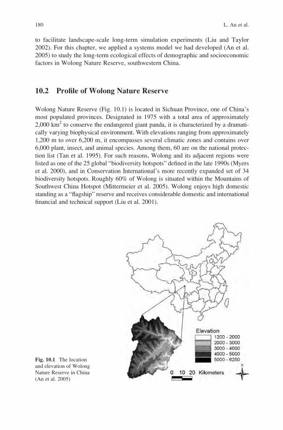
Wolong Nature Reserve (Fig. 10.1) is located in Sichuan Province, one of China’s

most populated provinces. Designated in 1975 with a total area of approximately

2,000 km2 to conserve the endangered giant panda, it is characterized by a dramati-

cally varying biophysical environment. With elevations ranging from approximately

1,200 m to over 6,200 m, it encompasses several climatic zones and contains over

6,000 plant, insect, and animal species. Among them, 60 are on the national protec-

tion list (Tan et al. 1995). For such reasons, Wolong and its adjacent regions were

listed as one of the 25 global “biodiversity hotspots” defined in the late 1990s (Myers

et al. 2000), and in Conservation International’s more recently expanded set of 34

biodiversity hotspots. Roughly 60% of Wolong is situated within the Mountains of

Southwest China Hotspot (Mittermeier et al. 2005). Wolong enjoys high domestic

standing as a “flagship” reserve and receives considerable domestic and international

financial and technical support (Liu et al. 2001).

Fig. 10.1 The location

and elevation of Wolong

Nature Reserve in China

(An et al. 2005)

180 L. An et al.

In 2000, approximately 4,413 farmers lived in the reserve, mostly along the sides

of the two main rivers running through the reserve; this population is made up of

four ethnic groups: Han, Tibetan, Qiang, and Hui (Liu et al. 1999a). Local residents

cut wood in the forests (on which pandas depend for habitat) for cooking and

heating their households in winter, using electricity mainly for lighting and elec-

tronic appliances. Only a small portion of the households uses electricity for

cooking and heating (An et al. 2001, 2002). No local market exists for fuelwood

transaction, and the farmers collect fuelwood primarily in winter for their own use

in the following year. Spending enormous amounts of time and energy for fuelwood

collection, local residents find it increasingly difficult to collect fuelwood due to the

shrinking forest area and topography characterized by high mountains and deep

valleys. The reserve administration has implemented many policies to restrict

fuelwood collection, including banning fuelwood collection in key habitat areas

and prohibiting some tree species from being harvested. Enforcement of these

fuelwood restriction policies tends to be ineffective because forests are a common

property and difficult to monitor, given the rugged terrain. Even though electricity

was available in the reserve, there was a continued increase in annual fuelwood

consumption (from 4,000 to 10,000 m3 from 1975 to 1999), contributing to a

reduction of over 20,000 ha of panda habitat (Liu et al. 1999b). Degradation of

forests and panda habitat was undoubtedly a factor in the reported decrease in panda

population, i.e., from 145 individuals in 1974 (Schaller et al. 1985) to 72 in 1986

(China’s Ministry of Forestry and World Wildlife Fund 1989).

The serious threat to the giant pandas comes from the subsistence needs of a fast

growing population experiencing dramatic changes in age structure and other

aspects. An even faster growth in household numbers may be contributing to the

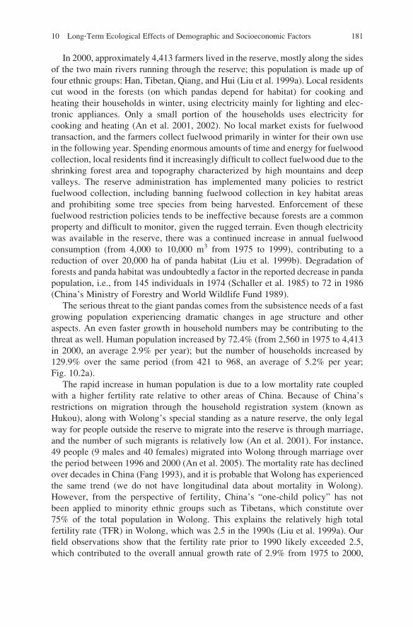
threat as well. Human population increased by 72.4% (from 2,560 in 1975 to 4,413

in 2000, an average 2.9% per year); but the number of households increased by

129.9% over the same period (from 421 to 968, an average of 5.2% per year;

Fig. 10.2a).

The rapid increase in human population is due to a low mortality rate coupled

with a higher fertility rate relative to other areas of China. Because of China’s

restrictions on migration through the household registration system (known as

Hukou), along with Wolong’s special standing as a nature reserve, the only legal

way for people outside the reserve to migrate into the reserve is through marriage,

and the number of such migrants is relatively low (An et al. 2001). For instance,

49 people (9 males and 40 females) migrated into Wolong through marriage over

the period between 1996 and 2000 (An et al. 2005). The mortality rate has declined

over decades in China (Fang 1993), and it is probable that Wolong has experienced

the same trend (we do not have longitudinal data about mortality in Wolong).

However, from the perspective of fertility, China’s “one-child policy” has not

been applied to minority ethnic groups such as Tibetans, which constitute over

75% of the total population in Wolong. This explains the relatively high total

fertility rate (TFR) in Wolong, which was 2.5 in the 1990s (Liu et al. 1999a). Our

field observations show that the fertility rate prior to 1990 likely exceeded 2.5,

which contributed to the overall annual growth rate of 2.9% from 1975 to 2000,

10 Long‐Term Ecological Effects of Demographic and Socioeconomic Factors 181

together with other influences, such as a higher proportion of young people reaching

the age of fertility during this period.

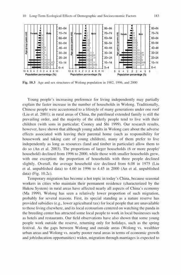
Previous research has shown that a change in the age structure could have a

significant impact on biodiversity: the more young adults living in Wolong, the

more forest may be cut down (Liu et al. 1999a). Average ages of local residents

increased from 1982 to 1996, with a decreased portion of the people belonging to

the 0–4, 5–9, and 10–14 age groups (Liu et al. 1999a; Wolong Nature Reserve 1997,

2000, Fig. 10.3). Changes between the 1996 and 2000 age structures were not as

obvious as those between 1982 and 1996, probably because of the shorter time

period. Overall, the groups that constitute the labor force (20–59 years) dominated

the local population, consistent with China’s general trend characterized by a

decreased proportion of children (0–14 years) and an increased proportion of

working-age (15–64 years) individuals (Hussain 2002). This decline was partly

due to the “later, longer, and fewer” (wan xi shao) family planning campaign,

encouraging or requiring couples to bear children later in life (later), prolonging the

time between the births of two consecutive children if more than one child is

allowed (longer), and having as few children as possible (fewer), which later

developed into the more strict “one-child policy” in most parts of China, especially

in cities (Feng and Hao 1992).

0

1000

2000

3000

4000

5000

1975 1980 1985 1990 1995 1999 2000

Year

Po

pu

lati

on

Siz

e

0

200

400

600

800

1000

1200

Nu

mb

er o

f H

ou

seh

old

s

Population Size

Number of Households

a

4.00

4.50

5.00

5.50

6.00

6.50

1970 1975 1980 1985 1990 1995 2000 2005

Year

Nu

mb

er o

f P

erso

ns

/ Ho

use

ho

ld

–50–40–30–20–1001020304050

1

2

3

4

5

Ed

uca

tio

n L

evel

s

Percentage (%)

Male Female

1996 2000

b c

Fig. 10.2 Population of Wolong Nature Reserve. (a) The dynamics of population size and the

number of households in Wolong between 1975 and 2000. (b) Education levels of Wolong

population in 1996 and 2000, where level 1 is for illiteracy, 2 for elementary school, 3 for middle

school, 4 for high school, and 5 for college, technical school, or higher. (c) Changes in household

size from 1975 to 2000

182 L. An et al.

Young people’s increasing preference for living independently may partially

explain the faster increase in the number of households in Wolong. Traditionally,

Chinese people were accustomed to a lifestyle of many generations under one roof

(Liu et al. 2001); in rural areas of China, the patrilineal extended family is still the

prevailing order, and the majority of the elderly people tend to live with their

children (with sons in particular; Cooney and Shi 1999). Our research results,

however, have shown that although young adults in Wolong care about the adverse

effects associated with leaving their parental home (such as responsibility for

housework and taking care of young children), many of them prefer to live

independently as long as resources (land and timber in particular) allow them to

do so (An et al. 2003). The proportions of larger households (6 or more people/

household) declined from 1996 to 2000, while those with smaller households grew,

with one exception: the proportion of households with three people declined

slightly. Overall, the average household size declined from 6.08 in 1975 (Liu

et al. unpublished data) to 4.60 in 1996 to 4.45 in 2000 (An et al. unpublished

data) (Fig. 10.2c).

Temporary migration has become a hot topic in today’s China, because seasonal

workers in cities who maintain their permanent residence (characterized by the

Hukou System) in rural areas have affected nearly all aspects of China’s economy

(Ma 1999). Wolong has seen a relatively lower proportion of such migration,

probably for several reasons. First, its special standing as a nature reserve has

provided subsidies (e.g., lower agricultural tax) for local people that are unavailable

to those living elsewhere, and its local ecotourism centered on watching the panda in

the breeding center has attracted some local people to work in local businesses such

as hotels and restaurants. Our field observations have also shown that some young

people work outside the reserve, returning only for holidays, such as the spring

festival. As the gaps between Wolong and outside areas (Wolong vs. wealthier

urban areas and Wolong vs. nearby poorer rural areas in terms of economic growth

and job/education opportunities) widen, migration through marriages is expected to

Fig. 10.3 Age and sex structures of Wolong population in 1982, 1996, and 2000


increase substantially. Therefore, we focus our concerns on migration through

marriages, despite their relatively low numbers in the recent past.1

Females had lower education levels than males: in both 1996 and 2000, a higher

proportion of females were at the illiterate level, and a lower proportion of females

belonged to each of the other levels (Fig. 10.2b). This suggests that girls did not

have the same chances for education as boys, probably due to the traditional

patrilineal extended family structure. The gender difference in education may

increase the probability that girls migrate out of Wolong through approaches

other than education-migration (i.e., moving out of Wolong through going to

college and finding jobs outside).

The pooled data (data for both females and males) show that the overall educa-

tion situation improved over time: illiteracy declined from 31% in 1982 (Liu et al.

1999a) to 28% in 1996 and to 25% in 2000. This change may indicate that in the

future, a higher proportion of children may pass the national college entrance

examinations, go to college, and settle down in cities after finding jobs there,

which could be a source of family pride for most of the parents in Wolong.

According to Liu et al. (2001), the vast majority of middle-aged and elderly

residents were not willing to move out of the reserve due to their low level of

educational attainment (Fig. 10.2b), difficulties in finding jobs in cities, and/or

difficulties in adapting to outside environment. However, they generally took

pride in their children and grandchildren doing so.

All such demographic and socioeconomic factors may affect panda habitat to

varying degrees, especially over a long time. Thus, it is very important to quantify

the magnitudes of changes in panda habitat (an indicator for local biodiversity)

caused by these factors. This chapter represents our attempt to examine the effects

of demographic and socioeconomic variables on panda habitat in the Wolong

Nature Reserve.

10.3 Long-Term Ecological Effects of Demographic

and Socioeconomic Factors

We are interested in how changes in the demographic features (e.g., age structure,

fertility) and socioeconomic conditions (electricity-related factors, particularly

because of electricity’s potential as a substitute for fuelwood) could affect panda

habitat over a long time in a spatially explicit manner. Major questions of interest

include (1) Which demographic and socioeconomic factors have significant (positive

or negative) impacts on panda habitat? (2) How could economic factors, such as an

electricity subsidy, conserve panda habitat? (3) How do spatiotemporal patterns of

1There were 49 (9 males and 40 females) people who migrated into and 67 (9 males and

58 females) people who migrated out of the reserve due to factors such as social networks

established by seasonal workers.

184 L. An et al.

panda habitat respond to changes in a combination of demographic and socioeco-

nomic factors?

10.3.1 Design of Simulation Experiments

To answer the above questions, we designed a set of simulation experiments to

understand how demographic and socioeconomic factors, when at play individu-

ally, would impact the two intermediate variables (population size and number of

households), and our ultimate state variable (panda habitat), over space and time

(Table 10.1). Through computer simulations, we tested a series of hypotheses

(presented in Table 10.1) regarding the impacts of demographic and socioeconomic

variables. First, for mortality and family planning factors, we examined the effects

of mortality rates. We assumed that Wolong had been going through the same

declining trend as the rest of China, reducing the mortality rates for all the six age

groups by 50%. Second, we varied the fertility from 2.0 (average number of

children allowed by the current policy in Wolong) to 1.0. This reduction is

consistent with the fact that although Wolong currently has a higher fertility rate

than cities in China, based on our field observations, many women in Wolong will

tend to have fewer children in the future. Third, we examined the effects of birth

interval by varying the length of birth interval (the time between the births of two

consecutive siblings) from 3.5 to 8 years, corresponding to the “longer” part of the

“fewer, longer, and later” family planning policy. Last, we examined the effects of

marriage age by varying this age from 22 to 32 years old, corresponding to the

“later” part of the policy.

To examine the effects of household formation and migration, we first evaluated

the effects of “leaving parental home intention”, the probability that a “parental-

home dweller” (an adult child who remains in his/her parental household after

marriage) would leave the parental household and set up a new household. We

reduced the intention from 0.42 to 0.05, to encourage young adult children not to

leave their parents’ homes after marriage, which would probably result in larger

household sizes and fewer households in the reserve. Second, we assessed the

effects of education emigration – the migration of young people, aged 16–20

years, to college and other educational institutions outside the reserve (An et al.

2001). We used a variable “college rate” to indicate the proportion of children

between 16 and 20 years old who could attend college. We varied the value of this

variable from 1.92% to 50%, representing a policy alternative that could encourage

more young people to move out of the reserve through approaches such as greater

investment in education. This policy would be socially acceptable, due to the

seniors’ support of their children or grandchildren’s outmigration to attend college

(see Sect. 10.2). Last, we examined the effects of marriage migration, represented

by a rise (from 0.28% to 50%) of “female marry-out rate”, the ratio of the females

between 22 and 30 years old who moved out of the reserve through marriage to all

the females in this age group at a given year (An et al. 2005).


Table

10.1

Designofsimulationexperim

ents

Typeoffactors

Variable

Hypothetical

impacta

Valueof

statusquo

Individual

experim

ent

Combined

experim

ent

Changed

value

Valueforconservation

scenario

Valuefordevelopment

scenario

Mortalityandfamily

planningfactors

Mortality

+Age dependentb

50% decrease

Fertility

�2.0

1.0

1.0

4

Birth

interval

+3.5

8.0

8.0

1.5

Marriageage

+22

32

32

22

Populationmovem

ent

factors

Leavingparentalhome

intention

�0.42

0.05

0.05

0.84

Collegerate

+1.92%

50%

50%

0.0%

Fem

alemarry-outrate

+0.28%

50%

50%

0.0%

Economic

factors

Electricity

Price

�Location

dependent

0.05Yuan

decline

0.05Yuan

decline

0.05Yuan

increase

Outagelevels

�Location

dependent

Onelevel

decrease

Onelevel

decrease

Onelevel

increase

Voltagelevels

+Location

dependent

Onelevel

increase

Onelevel

increase

Onelevel

decrease

aHypothesized

impactofadem

ographicorsocioeconomicvariableontheam

ountofpandahabitat.A“+

”signmeansthatachangein

thevalueofavariable

willchangetheam

ountofpandahabitat

inthesamedirection(e.g.,adecreasein

mortalitywillresultin

areductiononpandahabitat),whereasa“�

”sign

meansachangein

theopposite

direction(a

decreasein

fertilitywillgiverise

toan

increase

inpandahabitat)

bSee

Anet

al.(2005)fordetails

186 L. An et al.

To assess long-term effects of economic factors, we reduced the cost of electric-

ity by 0.05 Yuan kw�1 h�1 (US $1 ¼ 8.2 Yuan), reduced electricity outage by one

level,2 and increased voltage level by one level. These changes reflect the govern-

ment’s objectives of providing more high-quality electricity at a lower cost to

substitute for the use of fuelwood. An “eco-hydropower plant” was recently con-

structed to achieve these objectives (M. Liu personal communication).

To understand the combined effects of various factors on population size,

household numbers, and panda habitat, we designed a second set of simulation

experiments with two opposing scenarios. The “Conservation Scenario” combined

all the changes used in the above individual simulations that would help panda

habitat conservation through decreases in human population, number of house-

holds, and fuelwood consumption. The “Development Scenario” set the values of

all the related variables in the opposite direction (see Table 10.1), which would

stimulate development of local economy and growth of local population and house-

holds. We chose a simulation period of 20 years for the economic factors, while we

allowed demographic factors 30 years to take effect.

10.3.2 Model Description

To conduct the experiments outlined above, we used the Integrative Model for

Simulating Household and Ecosystem Dynamics (IMSHED; An et al. 2005), which

integrates various subsystems into a dynamic system that considers their interrela-

tionships and the underlying mechanisms of various interactions from a systems

perspective. IMSHED employs agent-based modeling (ABM) and geographic

information systems (GIS). ABM can help predict or explain emergent higher-

level phenomena by tracking the actions of multiple low-level “agents” that consti-

tute or at least impact the system behavior observed at higher levels. Agents usually

have some degree of self-awareness, intelligence, autonomous behavior, and

knowledge of the environment and other agents as well; they can adjust their own

actions in response to the changes in the environment and other agents (Lim et al.

2002). The model structure is illustrated in Fig. 10.4. IMSHED views individual

persons and households as discrete agents and land pixels as objects. The layer of

dashed households in the dashed box represents households at an earlier time, while

the layer of solid ones represents households at a later time.

2Electrical outages had three levels: high, moderate, and low, representing more than 5, 2–4, and

less than 2 outages per month, respectively. Voltage also had three levels, representing 220 V,

150–220 V, and fewer than 150 V (An et al. 2002). The default levels of outage and voltage for

each household in the model were based on real data: values for a given household could be any of

the three levels. If a specific household already has a low outage level, it would remain at that level

regardless of the request of reducing outage level. Households with moderate or high levels of

outage would have one level of reduction, resulting in low or moderate levels of outage,

respectively.


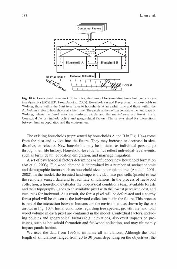
The existing households (represented by households A and B in Fig. 10.4) come

from the past and evolve into the future. They may increase or decrease in size,

dissolve, or relocate. New households may be initiated as individual persons go

through their life history. Household-level dynamics reflect individual-level events,

such as birth, death, education emigration, and marriage migration.

A set of psychosocial factors determines or influences new household formation

(An et al. 2003). Fuelwood demand is determined by a number of socioeconomic

and demographic factors such as household size and cropland area (An et al. 2001,

2002). In the model, the forested landscape is divided into grid cells (pixels) to use

the remotely sensed data and to facilitate simulations. In the process of fuelwood

collection, a household evaluates the biophysical conditions (e.g., available forests

and their topography), goes to an available pixel with the lowest perceived cost, and

cuts trees for fuelwood. As a result, the forest pixel will be deforested and a nearby

forest pixel will be chosen as the fuelwood collection site in the future. This process

is part of the interaction between humans and the environment, as shown by the two

arrows in Fig. 10.4. Initial conditions regarding tree species, growth rate, and total

wood volume in each pixel are contained in the model. Contextual factors, includ-

ing policies and geographical factors (e.g., elevation), also exert impacts on pro-

cesses, such as household formation and fuelwood collection, and may ultimately

impact panda habitat.

We used the data from 1996 to initialize all simulations. Although the total

length of simulations ranged from 20 to 30 years depending on the objectives, the

Forest

Household A

Contextual Factors

SPATIAL SCALETEMPORAL SCALE

Fuelwood Collection

Household B

Fig. 10.4 Conceptual framework of the integrative model for simulating household and ecosys-

tem dynamics (IMSHED; From An et al. 2005). Households A and B represent the households in

Wolong, those within the bold lines refer to households at an earlier time and those within the

dashed lines refer to households at a later time. The pixels at the bottom constitute the landscape of

Wolong, where the blank ones are nonforest pixels and the shaded ones are forest pixels.

Contextual factors include policy and geographical factors. The arrows stand for interactions

between human population and the environment

188 L. An et al.

simulation time step was always 1 year. The model contains many stochastic

processes, e.g., whether a person of a certain age group would survive a particular

year depends on the number generated by the random number generator: if it is less

than the associated yearly mortality rate, the person dies; otherwise he/she survives

and moves to the next year. We ran a simulation 30 times (or replicates) to capture

the variations among different replicates. We tested for the differences among

various simulation results using two-sample t tests at the 0.05 significance level.

10.3.3 Simulation Results

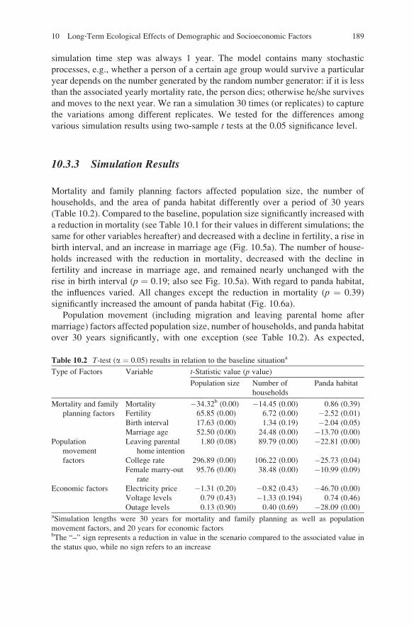
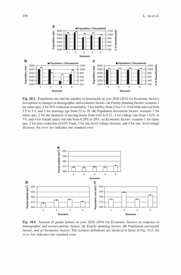
Mortality and family planning factors affected population size, the number of

households, and the area of panda habitat differently over a period of 30 years

(Table 10.2). Compared to the baseline, population size significantly increased with

a reduction in mortality (see Table 10.1 for their values in different simulations; the

same for other variables hereafter) and decreased with a decline in fertility, a rise in

birth interval, and an increase in marriage age (Fig. 10.5a). The number of house-

holds increased with the reduction in mortality, decreased with the decline in

fertility and increase in marriage age, and remained nearly unchanged with the

rise in birth interval (p ¼ 0.19; also see Fig. 10.5a). With regard to panda habitat,

the influences varied. All changes except the reduction in mortality (p ¼ 0.39)

significantly increased the amount of panda habitat (Fig. 10.6a).

Population movement (including migration and leaving parental home after

marriage) factors affected population size, number of households, and panda habitat

over 30 years significantly, with one exception (see Table 10.2). As expected,

Table 10.2 T-test (a ¼ 0.05) results in relation to the baseline situationa

Type of Factors Variable t-Statistic value (p value)

Population size Number of

households

Panda habitat

Mortality and family

planning factors

Mortality �34.32b (0.00) �14.45 (0.00) 0.86 (0.39)

Fertility 65.85 (0.00) 6.72 (0.00) �2.52 (0.01)

Birth interval 17.63 (0.00) 1.34 (0.19) �2.04 (0.05)

Marriage age 52.50 (0.00) 24.48 (0.00) �13.70 (0.00)

Population

movement

factors

Leaving parental

home intention

1.80 (0.08) 89.79 (0.00) �22.81 (0.00)

College rate 296.89 (0.00) 106.22 (0.00) �25.73 (0.04)

Female marry-out

rate

95.76 (0.00) 38.48 (0.00) �10.99 (0.09)

Economic factors Electricity price �1.31 (0.20) �0.82 (0.43) �46.70 (0.00)

Voltage levels 0.79 (0.43) �1.33 (0.194) 0.74 (0.46)

Outage levels 0.13 (0.90) 0.40 (0.69) �28.09 (0.00)aSimulation lengths were 30 years for mortality and family planning as well as population

movement factors, and 20 years for economic factorsbThe “–” sign represents a reduction in value in the scenario compared to the associated value in

the status quo, while no sign refers to an increase


560

570

580

590

600a

b c

1 2 3 4 5

Scenario

Pan

da

hab

itat

(km

2 )

Pan

da

hab

itat

(km

2 )

560

570

580

590

600

1 2 3 4

Scenario

560

570

580

590

600

1 2 3 4

Scenario

Po

pu

lati

on

siz

e (k

m2 )

Fig. 10.6 Amount of panda habitat in year 2026 (2016 for Economic factors) in response to

demographic and socioeconomic factors. (a) Family planning factors, (b) Population movement

factors, and (c) Economic factors. The scenario definitions are identical to those in Fig. 10.5. An

error bar indicates one standard error

1000

2000

3000

4000

5000

6000

1 2 3 4

1 2 3 4 1 2 3 4

5

ScenarioP

op

ula

tio

n s

ize

250

450

650

850

1050

1250

# o

f H

ou

seh

ou

lds

Population Household

1000

2000

3000

4000

5000

6000

Scenario

Po

pu

lati

on

siz

e

250

450

650

850

1050

1250Population Household

1000

2000

3000

4000

5000

6000

ScenarioP

op

ula

tio

n s

ize

250

450

650

850

1050

1250

# o

f H

ou

seh

ou

lds

Population Household

a

b c

Fig. 10.5 Population size and the number of households in year 2026 (2016 for Economic factors)

in response to changes in demographic and economic factors. (a) Family planning factors: scenario 1

for status quo, 2 for 50% reduction in mortality, 3 for fertility from 2.0 to 1.5, 4 for birth interval from

3.5 to 5.5, and 5 for marriage age from 22 to 28. (b) Population movement factors: scenario 1 for

status quo, 2 for the intention of leaving-home from 0.42 to 0.21, 3 for college rate from 1.92% to

5%, and 4 for female marry-out rate from 0.28% to 20%. (c) Economic factors: scenario 1 for status

quo, 2 for price reduction of 0.05 Yuan, 3 for one-level voltage increase, and 4 for onelevel outage

decrease. An error bar indicates one standard error

190 L. An et al.

the changes in the values of three population movement factors (a decrease in

leaving parental home intention, an increase in rate of college attendance, and an

increase in female marry-out rate) significantly reduced the number of households

(see Fig. 10.5b). Their influence on population size varied, however. Leaving

parental home had no statistically significant impact on population size (p ¼0.08), while an increase in rate of college attendance and female marry-out rate

significantly reduced population size (p <0.01). The amount of panda habitat

increased significantly (except for female marry-out rate with p ¼ 0.09) as a result

of increases in the values of all three factors (Fig. 10.6b).

The economic factors considered in our model had varying effects over a period

of 20 years (see Table 10.2). The three scenarios (a decrease in electricity price, an

increase in voltage level, and a decrease in the outage level) (see Fig. 10.5c)

had insignificant influences on population size. Similarly, their impact on the

number of households was insignificant. However, changes in the value of electric-

ity price and outage level increased panda habitat significantly, while a change in

the voltage level did not change the panda habitat significantly (p ¼ 0.46; also see

Fig. 10.6c).

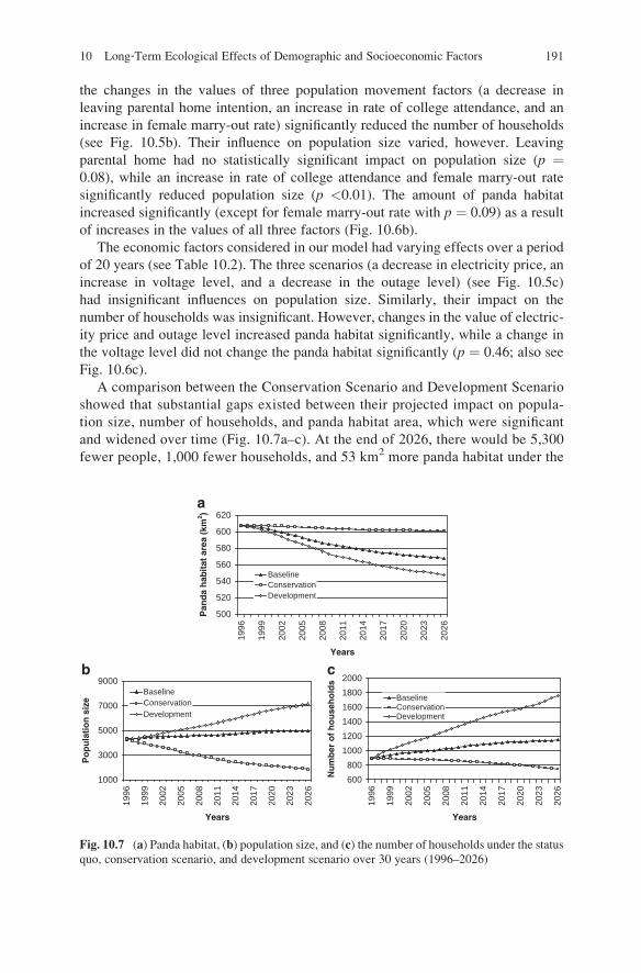
A comparison between the Conservation Scenario and Development Scenario

showed that substantial gaps existed between their projected impact on popula-

tion size, number of households, and panda habitat area, which were significant

and widened over time (Fig. 10.7a–c). At the end of 2026, there would be 5,300

fewer people, 1,000 fewer households, and 53 km2 more panda habitat under the

500

520

540

560

580

600

a620

1996

1999

2002

2005

2008

2011

2014

2017

2020

2023

2026

Years

Pan

da

hab

itat

are

a (k

m2 )

BaselineConservationDevelopment

b c

600

800

1000

1200

1400

1600

1800

2000

1996

1999

2002

2005

2008

2011

2014

2017

2020

2023

2026

Years

Nu

mb

er o

f h

ou

seh

old

s


1000

3000

5000

7000

9000

1996

1999

2002

2005

2008

2011

2014

2017

2020

2023

2026

Years

Po

pu

lati

on

siz

e


Fig. 10.7 (a) Panda habitat, (b) population size, and (c) the number of households under the status

quo, conservation scenario, and development scenario over 30 years (1996–2026)


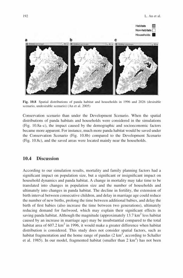
Conservation scenario than under the Development Scenario. When the spatial

distributions of panda habitats and households were considered in the simulations

(Fig. 10.8a–c), the impact caused by the demographic and socioeconomic factors

became more apparent. For instance, much more panda habitat would be saved under

the Conservation Scenario (Fig. 10.8b) compared to the Development Scenario

(Fig. 10.8c), and the saved areas were located mainly near the households.

10.4 Discussion

According to our simulation results, mortality and family planning factors had a

significant impact on population size, but a significant or insignificant impact on

household dynamics and panda habitat. A change in mortality may take time to be

translated into changes in population size and the number of households and

ultimately into changes in panda habitat. The decline in fertility, the extension of

birth interval between consecutive children, and delay in marriage age could reduce

the number of new births, prolong the time between additional babies, and delay the

birth of first babies (also increase the time between two generations), ultimately

reducing demand for fuelwood, which may explain their significant effects in

saving panda habitat. Although the magnitude (approximately 13.7 km2 less habitat

caused by an increase in marriage age) may be insubstantial compared to the total

habitat area of 607.2 km2 in 1996, it would make a greater difference when habitat

distribution is considered. This study does not consider spatial factors, such as

habitat fragmentation and the home range of pandas (2 km2, according to Schaller

et al. 1985). In our model, fragmented habitat (smaller than 2 km2) has not been

Fig. 10.8 Spatial distributions of panda habitat and households in 1996 and 2026 (desirable

scenario, undesirable scenario) (An et al. 2005)

192 L. An et al.

taken out. Thus, if a habitat of 100 km2, for instance, were divided into small

fragments of less than 2 km2 each, the real loss would be 100 km2 rather than zero.

Factors influencing population movement affected nearly all three response

variables: population size, household numbers, and panda habitat. There were

two exceptions: leaving-home intention and female marry-out rate showed no

statistically significant effect on population size and panda habitat at the 0.05

significance level. Leaving-home intention largely deals with how likely it would

be for a newly married couple to establish their own household, and it is not directly

linked to population size. The female marry-out rate may need more time (i.e.,

longer than 30 years) to affect population size, household numbers, and, ultimately,

panda habitat.

Economic factors had a significant impact on panda habitat because they

encourage local residents to reduce their consumption of fuelwood by using more

electricity. The Conservation Scenario and Development Scenario shed light on

how demographic factors (especially those linked to population structure) and

socioeconomic factors may influence panda habitat over time, illustrating substan-

tial temporal and spatial differences in response to two opposite combinations of

variables.

The results from our simulation study have important implications for the

development of feasible and effective conservation policies. For example, promot-

ing outmigration of young people through college education is not only socially

desirable (Liu et al. 1999b), but also ecologically effective. Providing cheaper,

more reliable, and higher-quality electricity for local residents could help them

switch from fuelwood consumption to electricity use. A lesser dependence on

fuelwood could help protect and restore panda habitat.

Future research should be directed towards the following aspects. First, it

is necessary to collect more data (both cross-sectional and longitudinal) at the

household level concerning demographic features, household economy (income

and expenditures, material input/output), new household establishment, migra-

tion, and locations of both new households and fuelwood collection sites. These

data could allow us to test hypotheses more rigorously in terms of plausible causal

relationships (e.g., females’ lower education could cause higher female out-

migration through marriage). Such studies would not only be important to social

scientists but could also be used to explain the dynamics of local biodiversity

(represented by panda habitat in our study).

The impact of mortality and family planning factors on panda habitat may not be

apparent for many years, as exemplified by the effects of an increase in marriage

age on panda habitat. Thus, long-term studies of the factors presented in this chapter

are essential. Spatial ABM (usually coupled with GIS) provides researchers with a

useful tool to capture and integrate various detailed data – rather than just the

averages – into a systems framework and overcome the shortcomings of traditional

equation-based models. We conclude that this powerful experimental tool can

promote a more complete understanding of long-term biodiversity dynamics across

human-influenced landscapes.


Acknowledgments We thank Wolong Nature Reserve, especially Director Hemin Zhang for

logistic assistance in field work and Jinyan Huang and Shiqiang Zhou for their assistance in data

acquisition. We appreciate the valuable comments and edits from Richard Cincotta, Larry Goren-

flo, and three anonymous reviewers. For financial support, we are indebted to the US National

Science Foundation (NSF), US National Institutes of Health (NIH), American Association for

Advancement of Sciences, John D. and Catherine T. MacArthur Foundation, and National Natural

Science Foundation of China.

References

An L, Liu J, Ouyang Z, Linderman MA, Zhou S, Zhang H (2001) Simulating demographic and

socioeconomic processes on household level and implications on giant panda habitat. Ecol

Model 140:31–49

An L, Lupi F, Liu J, Linderman MA, Huang J (2002) Modeling the choice to switch from fuelwood

to electricity: implications for giant panda habitat conservation. Ecol Econ 42(3):445–457

An L, Mertig A, Liu J (2003) Adolescents’ leaving parental home: psychosocial correlates and

implications for biodiversity conservation. Popul Environ 24(5):415–444

An L, Linderman MA, Shortridge A, Qi J, Liu J (2005) Exploring complexity in a human-

environment system: an agent-based spatial model for multidisciplinary and multi-scale

integration. Ann Assoc Am Geogr 95(1):54–79

Brashares JS, Arcese P, Sam MK (2001) Human demography and reserve size predict wildlife

extinction in West Africa. Proc R Soc Lond Ser B Biol Sci 268(1484):2473–2478

China’s Ministry of Forestry and World Wildlife Fund (1989) Conservation and management plan

for Giant Pandas and their habitat. China’s Ministry of Forestry and World Wildlife Fund,

Beijing

Cincotta RP, Wisnewski J, Engelman R (2000) Human population in the biodiversity hotspots.

Nature 404:990–992

Cooney RS, Shi J (1999) Household extension of the elderly in China, 1987. Popul Res Policy Rev

18(5):451–471

Fang RK (1993) The geographical inequalities of mortality in China. Social Sci Med 36(10):

1319–1323

Feng G, Hao L (1992) Summary of 28 regional birth planning regulations in China. Popul Res

(Renkou Yanjiu; in Chinese) 4:28–33

Forester DJ, Machlis GE (1996) Modeling human factors that affect the loss of biodiversity.

Conserv Biol 10(4):1253–1263

Hussain A (2002) Demographic transition in China and its implication. World Dev 30(10):

1823–1834

Lim K, Deadman PJ, Moran E, Brondizio E, McCracken S (2002) Agent-based simulations of

household decision-making and land use change near Altamira, Brazil. In: Gimblett HR (ed)

Integrating geographic information systems and agent-based techniques for simulating social

and ecological processes. Oxford University Press, New York, pp 277–308

Liu J, Taylor WW (eds) (2002) Integrating landscape ecology into natural resource management.

Cambridge University Press, Cambridge, UK

Liu J, Ouyang Z, Tan Y, Yang J, Zhang H (1999a) Changes in human population structure:

implications for biodiversity. Popul Environ 21:46–58

Liu J, Ouyang Z, Taylor WW, Groop R, Zhang H (1999b) A framework for evaluating the effects

of human factors ob wildlife habitat: the case of giant pandas. Conserv Biol 13:1360–1370

Liu J, Linderman M, Ouyang Z, An L, Yang J, Zhang H (2001) Ecological degradation in

protected areas: the case of Wolong Nature Reserve for giant pandas. Science 292:98–101

Liu J, Daily GC, Ehrlich PR, Luck GW (2003) Effects of household dynamics on resource

consumption and biodiversity. Nature 421(6922):530–533

194 L. An et al.

Ma Z (1999) Temporary migration and regional development in China. Environ Plann A

31:783–802

McKee JK, Sciulli PW, Fooce CD, Waite TA (2004) Forecasting global biodiversity threats

associated with human population growth. Biol Conserv 115(1):161–164

Mittermeier RA, Gil PR, Hoffman M, Pilgrim J, Brooks T, Mittermeier CG, Lamoreux J, da

Fonseca GAB (2005) Hotspots revisited. Conservation International, Washington, DC

Myers N, Mittermeier RA, Mittermeier CG, da Fonseca GAB, Kent J (2000) Biodiversity hotspots

for conservation priorities. Nature 403:853–858

Schaller GB, Hu J, Pan W, Zhu J (1985) The giant pandas of Wolong. University of Chicago Press,

Chicago and London

Tan Y, Ouyang Z, Zhang H (1995) Spatial characteristics of biodiversity in Wolong Nature

Reserve. China’s Biodiversity Reserve 3:19–24 (in Chinese)

Veech JA (2003) Incorporating socioeconomic factors into the analysis of biodiversity hotspots.

Appl Geogr 23(1):73–88

Wolong Nature Reserve (1997) Wolong Agricultural Operation and Contracting Situations

(unpublished, in Chinese)

Wolong Nature Reserve (2000) Wolong 2000 Nationwide Population Census Form (unpublished,

in Chinese)


Documents

Chapter 10 Long-Term Ecological Effects of …csis.msu.edu/sites/csis.msu.edu/files/Chapter_10.pdfChapter 10 Long-Term Ecological Effects of Demographic and Socioeconomic Factors in