Embed Size (px)
Citation preview
Shiqian Ma, MAT-258A: Numerical Optimization 1
Chapter 10
(Block) Coordinate Descent Method
Shiqian Ma, MAT-258A: Numerical Optimization 2
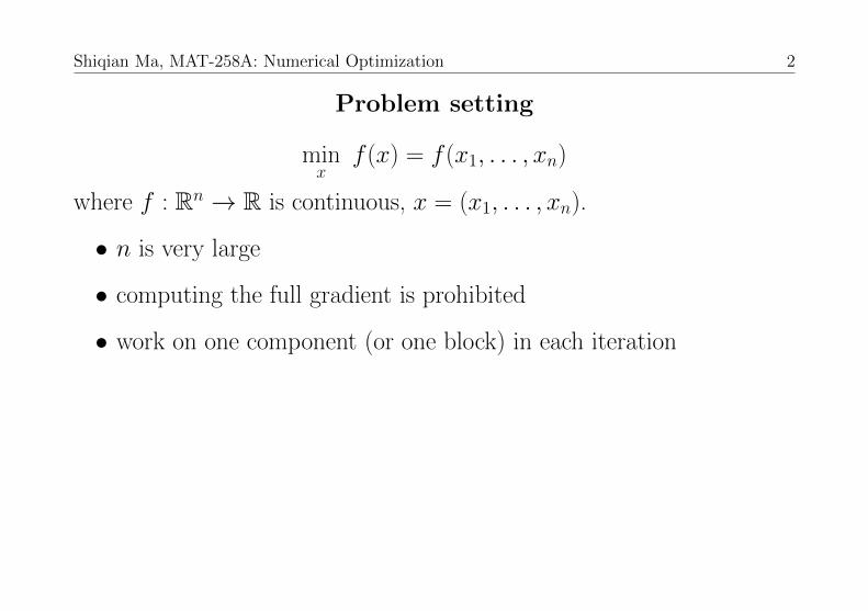
Problem setting
minx
f (x) = f (x1, . . . , xn)
where f : Rn → R is continuous, x = (x1, . . . , xn).
• n is very large
• computing the full gradient is prohibited
• work on one component (or one block) in each iteration
Shiqian Ma, MAT-258A: Numerical Optimization 3
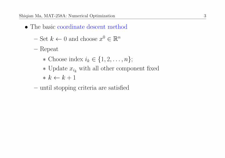
• The basic coordinate descent method
– Set k ← 0 and choose x0 ∈ Rn
– Repeat
∗ Choose index ik ∈ 1, 2, . . . , n;∗ Update xik with all other component fixed
∗ k ← k + 1
– until stopping criteria are satisfied
Shiqian Ma, MAT-258A: Numerical Optimization 4
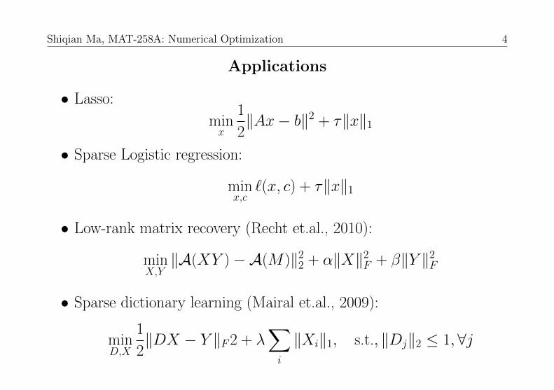
Applications
• Lasso:
minx
1
2‖Ax− b‖2 + τ‖x‖1
• Sparse Logistic regression:
minx,c
`(x, c) + τ‖x‖1
• Low-rank matrix recovery (Recht et.al., 2010):
minX,Y‖A(XY )−A(M)‖22 + α‖X‖2F + β‖Y ‖2F
• Sparse dictionary learning (Mairal et.al., 2009):
minD,X
1
2‖DX − Y ‖F2 + λ
∑i
‖Xi‖1, s.t., ‖Dj‖2 ≤ 1,∀j
Shiqian Ma, MAT-258A: Numerical Optimization 5
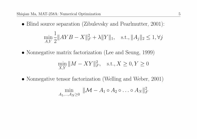
• Blind source separation (Zibulevsky and Pearlmutter, 2001):
minA,Y
1
2‖AY B −X‖2F + λ‖Y ‖1, s.t., ‖Aj‖2 ≤ 1,∀j
• Nonnegative matrix factorization (Lee and Seung, 1999)
minX,Y‖M −XY ‖2F , s.t., X ≥ 0, Y ≥ 0
• Nonnegative tensor factorization (Welling and Weber, 2001)
minA1,...,AN≥0
‖M− A1 A2 . . . AN‖2F
Shiqian Ma, MAT-258A: Numerical Optimization 6
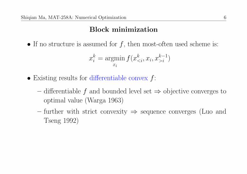
Block minimization
• If no structure is assumed for f , then most-often used scheme is:
xki = argminxi
f (xk<i, xi, xk−1>i )
• Existing results for differentiable convex f :
– differentiable f and bounded level set ⇒ objective converges to
optimal value (Warga 1963)
– further with strict convexity ⇒ sequence converges (Luo and
Tseng 1992)
Shiqian Ma, MAT-258A: Numerical Optimization 7
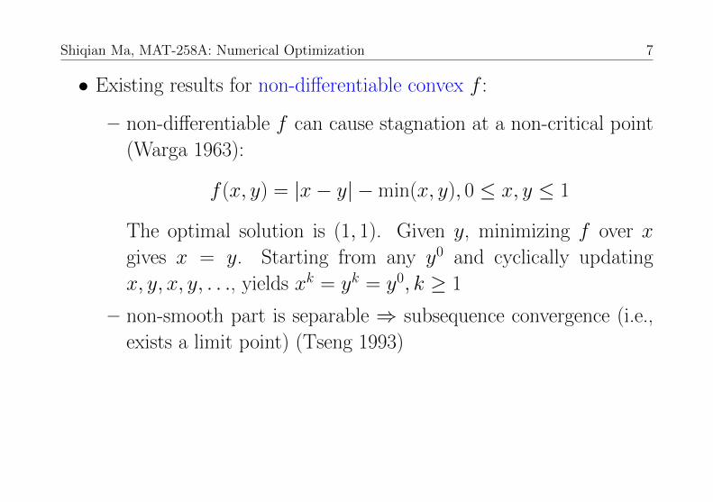
• Existing results for non-differentiable convex f :
– non-differentiable f can cause stagnation at a non-critical point
(Warga 1963):
f (x, y) = |x− y| −min(x, y), 0 ≤ x, y ≤ 1
The optimal solution is (1, 1). Given y, minimizing f over x
gives x = y. Starting from any y0 and cyclically updating
x, y, x, y, . . ., yields xk = yk = y0, k ≥ 1
– non-smooth part is separable ⇒ subsequence convergence (i.e.,
exists a limit point) (Tseng 1993)
Shiqian Ma, MAT-258A: Numerical Optimization 8
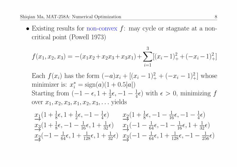
• Existing results for non-convex f : may cycle or stagnate at a non-
critical point (Powell 1973)
f (x1, x2, x3) = −(x1x2 +x2x3 +x3x1) +
3∑i=1
[(xi−1)2+ + (−xi−1)2+]
Each f (xi) has the form (−a)xi + [(xi − 1)2+ + (−xi − 1)2+] whose
minimizer is: x∗i = sign(a)(1 + 0.5|a|)Starting from (−1 − ε, 1 + 1
2ε,−1 − 14ε) with ε > 0, minimizing f
over x1, x2, x3, x1, x2, x3, . . . yields
x1−→(1 + 18ε, 1 + 1
2ε,−1− 14ε) x2−→(1 + 1
8ε,−1− 116ε,−1− 1
4ε)
x3−→(1 + 18ε,−1− 1
16ε, 1 + 132ε) x1−→(−1− 1
64ε,−1− 116ε, 1 + 1
32ε)
x2−→(−1− 164ε, 1 + 1
128ε, 1 + 132ε) x3−→(−1− 1
64ε, 1 + 1128ε,−1− 1
256ε)
Shiqian Ma, MAT-258A: Numerical Optimization 9
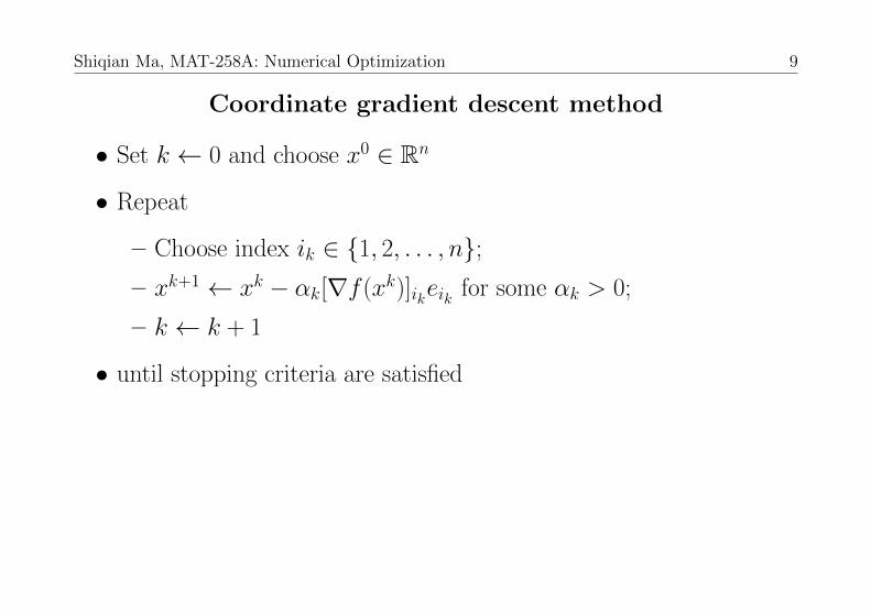
Coordinate gradient descent method
• Set k ← 0 and choose x0 ∈ Rn
• Repeat
– Choose index ik ∈ 1, 2, . . . , n;– xk+1 ← xk − αk[∇f (xk)]ikeik for some αk > 0;
– k ← k + 1
• until stopping criteria are satisfied
Shiqian Ma, MAT-258A: Numerical Optimization 10
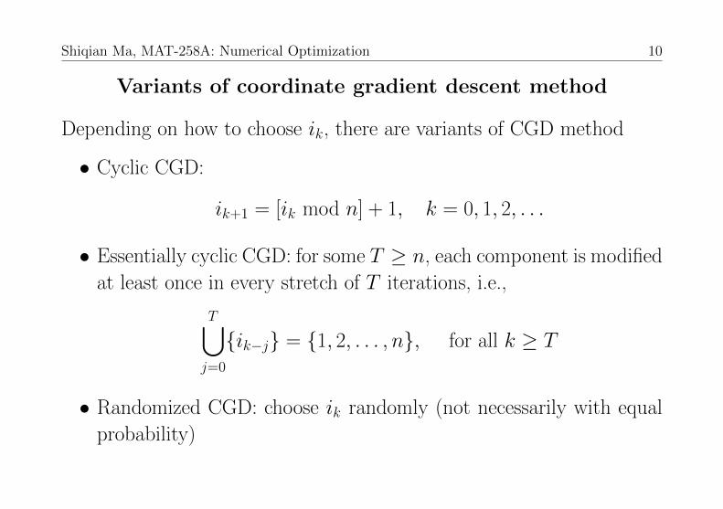
Variants of coordinate gradient descent method
Depending on how to choose ik, there are variants of CGD method
• Cyclic CGD:
ik+1 = [ik mod n] + 1, k = 0, 1, 2, . . .
• Essentially cyclic CGD: for some T ≥ n, each component is modified
at least once in every stretch of T iterations, i.e.,
T⋃j=0
ik−j = 1, 2, . . . , n, for all k ≥ T
• Randomized CGD: choose ik randomly (not necessarily with equal
probability)

Shiqian Ma, MAT-258A: Numerical Optimization 11
How to choose αk
Through one of the following alternatives:
• perform exact minimization along the ik component
• choose αk that satisfies some line-search conditions
• choose αk based on prior knowledge of properties of f
Shiqian Ma, MAT-258A: Numerical Optimization 12
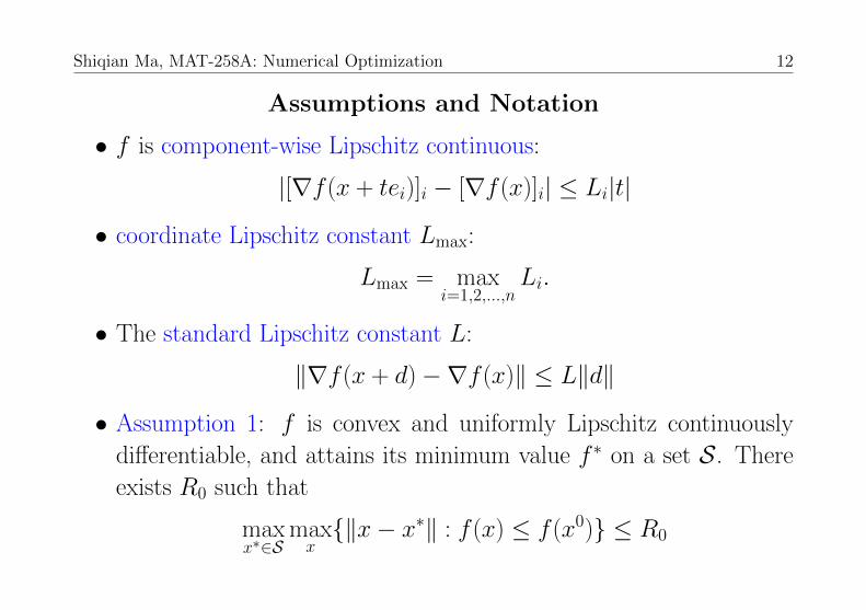
Assumptions and Notation
• f is component-wise Lipschitz continuous:
|[∇f (x + tei)]i − [∇f (x)]i| ≤ Li|t|
• coordinate Lipschitz constant Lmax:
Lmax = maxi=1,2,...,n
Li.
• The standard Lipschitz constant L:
‖∇f (x + d)−∇f (x)‖ ≤ L‖d‖
• Assumption 1: f is convex and uniformly Lipschitz continuously
differentiable, and attains its minimum value f ∗ on a set S . There
exists R0 such that
maxx∗∈S
maxx‖x− x∗‖ : f (x) ≤ f (x0) ≤ R0
Shiqian Ma, MAT-258A: Numerical Optimization 13
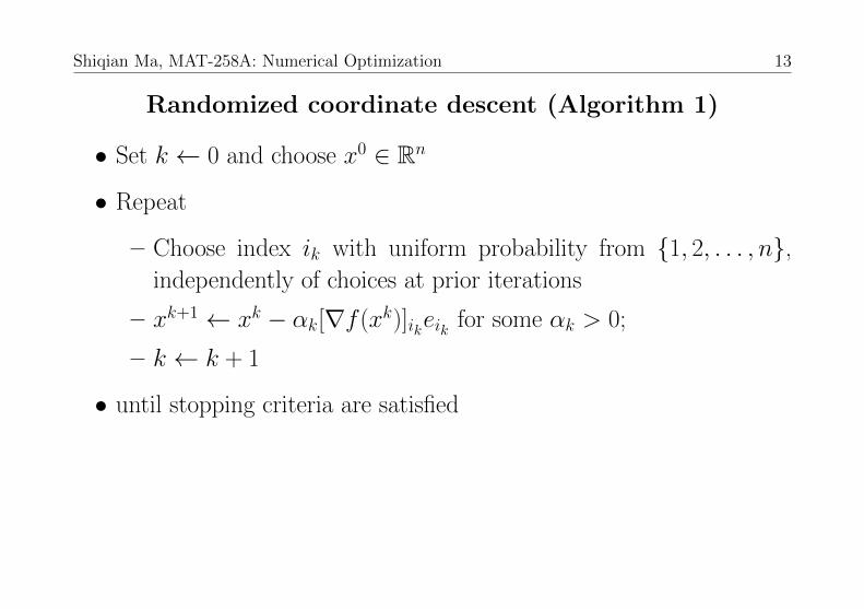
Randomized coordinate descent (Algorithm 1)
• Set k ← 0 and choose x0 ∈ Rn
• Repeat
– Choose index ik with uniform probability from 1, 2, . . . , n,independently of choices at prior iterations
– xk+1 ← xk − αk[∇f (xk)]ikeik for some αk > 0;
– k ← k + 1
• until stopping criteria are satisfied
Shiqian Ma, MAT-258A: Numerical Optimization 14
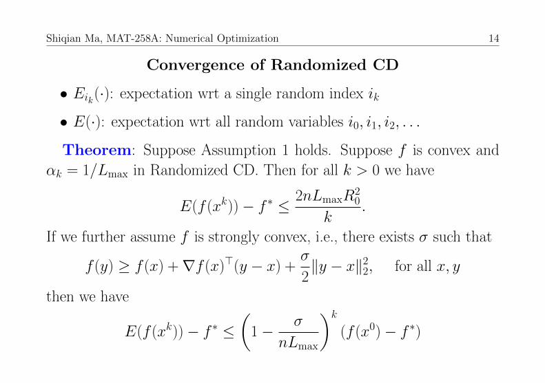
Convergence of Randomized CD
• Eik(·): expectation wrt a single random index ik
• E(·): expectation wrt all random variables i0, i1, i2, . . .
Theorem: Suppose Assumption 1 holds. Suppose f is convex and
αk = 1/Lmax in Randomized CD. Then for all k > 0 we have
E(f (xk))− f ∗ ≤ 2nLmaxR20
k.
If we further assume f is strongly convex, i.e., there exists σ such that
f (y) ≥ f (x) +∇f (x)>(y − x) +σ
2‖y − x‖22, for all x, y
then we have
E(f (xk))− f ∗ ≤(
1− σ
nLmax
)k(f (x0)− f ∗)
Shiqian Ma, MAT-258A: Numerical Optimization 15
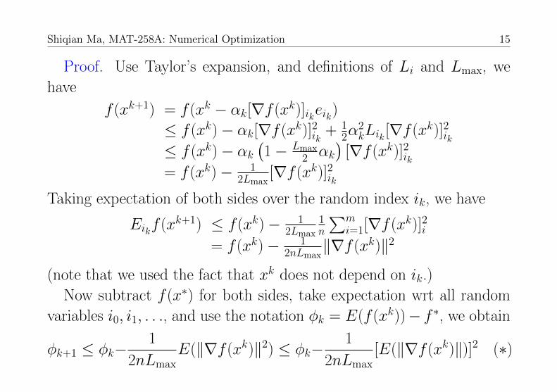
Proof. Use Taylor’s expansion, and definitions of Li and Lmax, we
have
f (xk+1) = f (xk − αk[∇f (xk)]ikeik)
≤ f (xk)− αk[∇f (xk)]2ik + 12α
2kLik [∇f (xk)]2ik
≤ f (xk)− αk(1− Lmax
2 αk)
[∇f (xk)]2ik= f (xk)− 1
2Lmax[∇f (xk)]2ik
Taking expectation of both sides over the random index ik, we have
Eikf (xk+1) ≤ f (xk)− 12Lmax
1n
∑mi=1[∇f (xk)]2i
= f (xk)− 12nLmax
‖∇f (xk)‖2
(note that we used the fact that xk does not depend on ik.)
Now subtract f (x∗) for both sides, take expectation wrt all random
variables i0, i1, . . ., and use the notation φk = E(f (xk))− f ∗, we obtain
φk+1 ≤ φk−1
2nLmaxE(‖∇f (xk)‖2) ≤ φk−
1
2nLmax[E(‖∇f (xk)‖)]2 (∗)
Shiqian Ma, MAT-258A: Numerical Optimization 16
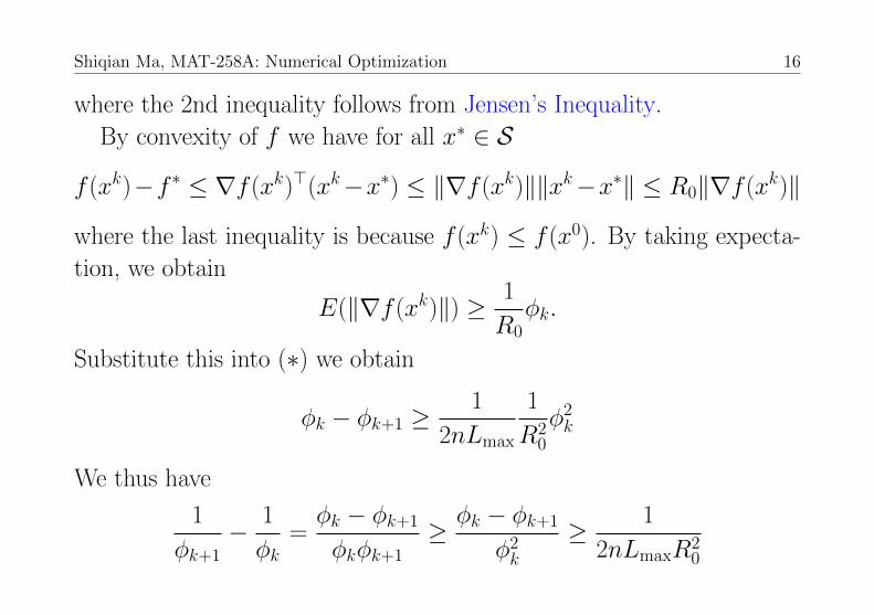
where the 2nd inequality follows from Jensen’s Inequality.
By convexity of f we have for all x∗ ∈ S
f (xk)−f ∗ ≤ ∇f (xk)>(xk−x∗) ≤ ‖∇f (xk)‖‖xk−x∗‖ ≤ R0‖∇f (xk)‖
where the last inequality is because f (xk) ≤ f (x0). By taking expecta-
tion, we obtain
E(‖∇f (xk)‖) ≥ 1
R0φk.
Substitute this into (∗) we obtain
φk − φk+1 ≥1
2nLmax
1
R20
φ2k
We thus have
1
φk+1− 1
φk=φk − φk+1
φkφk+1≥ φk − φk+1
φ2k≥ 1
2nLmaxR20
Shiqian Ma, MAT-258A: Numerical Optimization 17
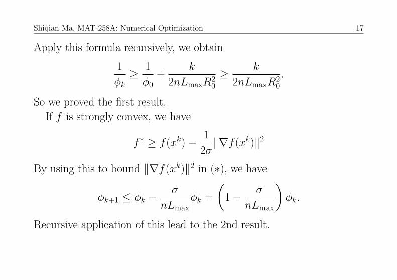
Apply this formula recursively, we obtain
1
φk≥ 1
φ0+
k
2nLmaxR20
≥ k
2nLmaxR20
.
So we proved the first result.
If f is strongly convex, we have
f ∗ ≥ f (xk)− 1
2σ‖∇f (xk)‖2
By using this to bound ‖∇f (xk)‖2 in (∗), we have
φk+1 ≤ φk −σ
nLmaxφk =
(1− σ
nLmax
)φk.
Recursive application of this lead to the 2nd result.
Shiqian Ma, MAT-258A: Numerical Optimization 18
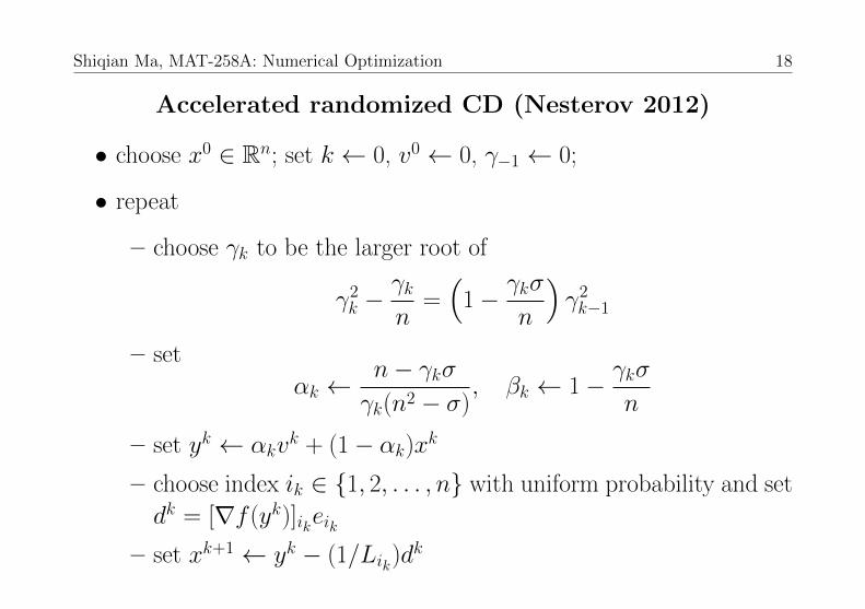
Accelerated randomized CD (Nesterov 2012)
• choose x0 ∈ Rn; set k ← 0, v0 ← 0, γ−1 ← 0;
• repeat
– choose γk to be the larger root of
γ2k −γkn
=(
1− γkσ
n
)γ2k−1
– set
αk ←n− γkσγk(n2 − σ)
, βk ← 1− γkσ
n
– set yk ← αkvk + (1− αk)xk
– choose index ik ∈ 1, 2, . . . , n with uniform probability and set
dk = [∇f (yk)]ikeik– set xk+1 ← yk − (1/Lik)d
k
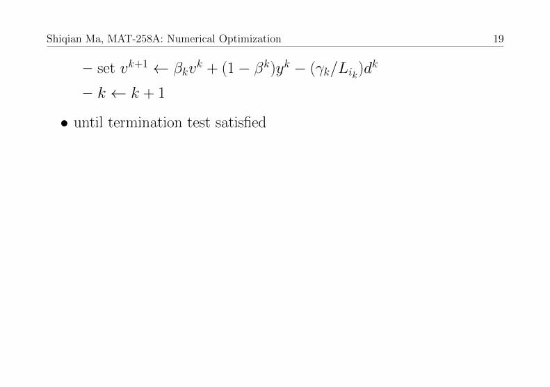
Shiqian Ma, MAT-258A: Numerical Optimization 19
– set vk+1 ← βkvk + (1− βk)yk − (γk/Lik)d
k
– k ← k + 1
• until termination test satisfied
Shiqian Ma, MAT-258A: Numerical Optimization 20
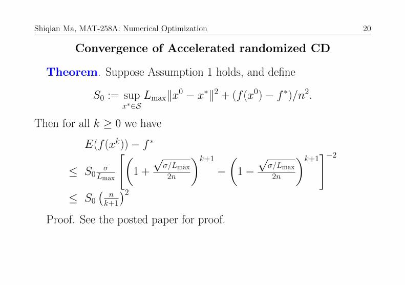
Convergence of Accelerated randomized CD
Theorem. Suppose Assumption 1 holds, and define
S0 := supx∗∈S
Lmax‖x0 − x∗‖2 + (f (x0)− f ∗)/n2.
Then for all k ≥ 0 we have
E(f (xk))− f ∗
≤ S0σ
Lmax
[(1 +
√σ/Lmax
2n
)k+1
−(
1−√σ/Lmax
2n
)k+1]−2
≤ S0
(nk+1
)2Proof. See the posted paper for proof.
Shiqian Ma, MAT-258A: Numerical Optimization 21
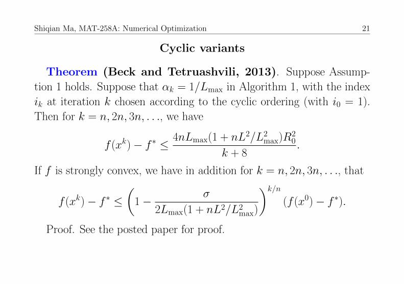
Cyclic variants
Theorem (Beck and Tetruashvili, 2013). Suppose Assump-
tion 1 holds. Suppose that αk = 1/Lmax in Algorithm 1, with the index
ik at iteration k chosen according to the cyclic ordering (with i0 = 1).
Then for k = n, 2n, 3n, . . ., we have
f (xk)− f ∗ ≤ 4nLmax(1 + nL2/L2max)R
20
k + 8.
If f is strongly convex, we have in addition for k = n, 2n, 3n, . . ., that
f (xk)− f ∗ ≤(
1− σ
2Lmax(1 + nL2/L2max)
)k/n(f (x0)− f ∗).
Proof. See the posted paper for proof.
Shiqian Ma, MAT-258A: Numerical Optimization 22
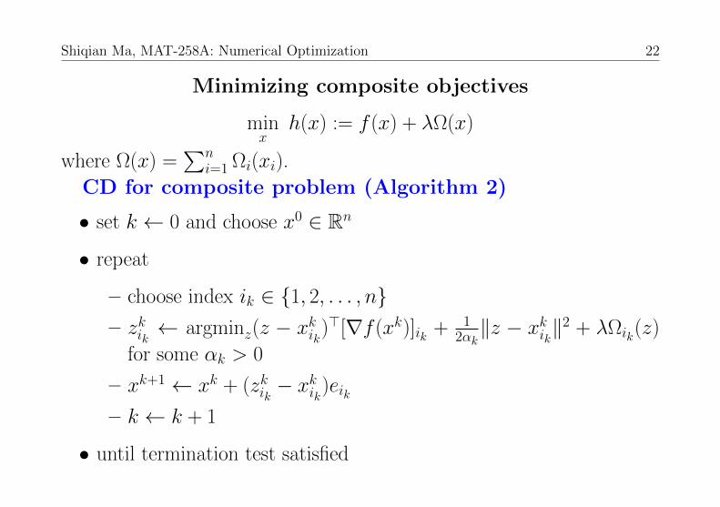
Minimizing composite objectives
minx
h(x) := f (x) + λΩ(x)
where Ω(x) =∑n
i=1 Ωi(xi).
CD for composite problem (Algorithm 2)
• set k ← 0 and choose x0 ∈ Rn
• repeat
– choose index ik ∈ 1, 2, . . . , n– zkik ← argminz(z − xkik)
>[∇f (xk)]ik + 12αk‖z − xkik‖
2 + λΩik(z)
for some αk > 0
– xk+1 ← xk + (zkik − xkik
)eik– k ← k + 1
• until termination test satisfied
Shiqian Ma, MAT-258A: Numerical Optimization 23
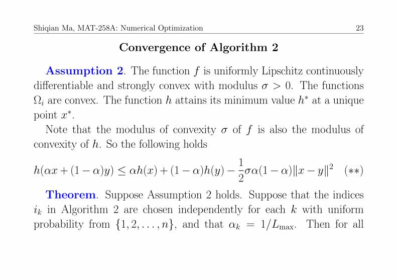
Convergence of Algorithm 2
Assumption 2. The function f is uniformly Lipschitz continuously
differentiable and strongly convex with modulus σ > 0. The functions
Ωi are convex. The function h attains its minimum value h∗ at a unique
point x∗.
Note that the modulus of convexity σ of f is also the modulus of
convexity of h. So the following holds
h(αx+ (1−α)y) ≤ αh(x) + (1−α)h(y)− 1
2σα(1−α)‖x− y‖2 (∗∗)
Theorem. Suppose Assumption 2 holds. Suppose that the indices
ik in Algorithm 2 are chosen independently for each k with uniform
probability from 1, 2, . . . , n, and that αk = 1/Lmax. Then for all
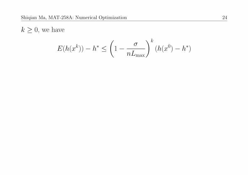
Shiqian Ma, MAT-258A: Numerical Optimization 24
k ≥ 0, we have
E(h(xk))− h∗ ≤(
1− σ
nLmax
)k(h(x0)− h∗)
Shiqian Ma, MAT-258A: Numerical Optimization 25
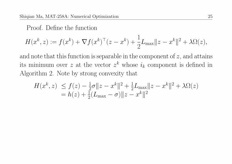
Proof. Define the function
H(xk, z) := f (xk) +∇f (xk)>(z − xk) +1
2Lmax‖z − xk‖2 + λΩ(z),
and note that this function is separable in the component of z, and attains
its minimum over z at the vector zk whose ik component is defined in
Algorithm 2. Note by strong convexity that
H(xk, z) ≤ f (z)− 12σ‖z − x
k‖2 + 12Lmax‖z − xk‖2 + λΩ(z)
= h(z) + 12(Lmax − σ)‖z − xk‖2
Shiqian Ma, MAT-258A: Numerical Optimization 26
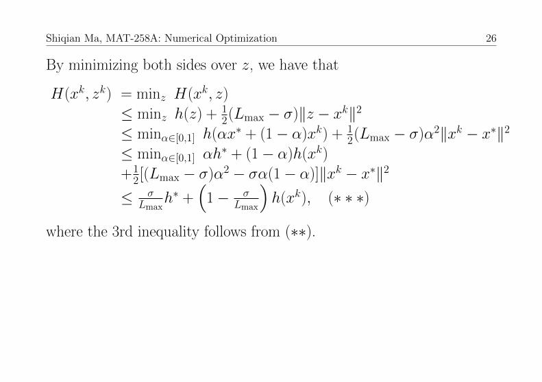
By minimizing both sides over z, we have that
H(xk, zk) = minz H(xk, z)
≤ minz h(z) + 12(Lmax − σ)‖z − xk‖2
≤ minα∈[0,1] h(αx∗ + (1− α)xk) + 12(Lmax − σ)α2‖xk − x∗‖2
≤ minα∈[0,1] αh∗ + (1− α)h(xk)
+12[(Lmax − σ)α2 − σα(1− α)]‖xk − x∗‖2
≤ σLmax
h∗ +(
1− σLmax
)h(xk), (∗ ∗ ∗)
where the 3rd inequality follows from (∗∗).
Shiqian Ma, MAT-258A: Numerical Optimization 27
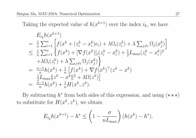
Taking the expected value of h(xk+1) over the index ik, we have
Eikh(xk+1)
= 1n
∑ni=1
[f (xk + (zki − xki )ei) + λΩi(z
ki ) + λ
∑j 6=i Ωj(x
kj )]
≤ 1n
∑ni=1
f (xk) + [∇f (xk)]i(z
ki − xki ) + 1
2Lmax(zki − xki )2
+λΩi(zki ) + λ
∑j 6=i Ωj(x
kj )
= n−1n h(xk) + 1
n
[f (xk) +∇f (xk)>(zk − xk)
12Lmax‖zk − xk‖2 + λΩ(zk)
]= n−1
n h(xk) + 1nH(xk, zk).
By subtracting h∗ from both sides of this expression, and using (∗∗∗)to substitute for H(xk, zk), we obtain
Eikh(xk+1)− h∗ ≤(
1− σ
nLmax
)(h(xk)− h∗).
Shiqian Ma, MAT-258A: Numerical Optimization 28
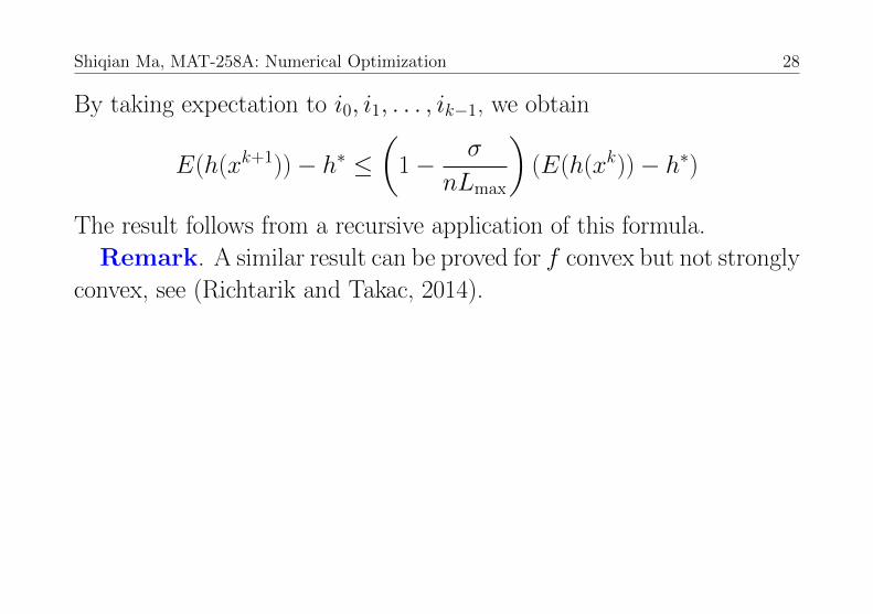
By taking expectation to i0, i1, . . . , ik−1, we obtain
E(h(xk+1))− h∗ ≤(
1− σ
nLmax
)(E(h(xk))− h∗)
The result follows from a recursive application of this formula.
Remark. A similar result can be proved for f convex but not strongly
convex, see (Richtarik and Takac, 2014).
Shiqian Ma, MAT-258A: Numerical Optimization 29
Maximum Block Improvement (MBI) Method
Solve(G) max f (x1, x2, . . . , xd)
s.t. xi ∈ Si ⊂ Rni, i = 1, 2, . . . , d
f can be nonconvex.
• Note that for nonconvex problem, the usual BCD is not necessarily
convergent.
• The idea of MBI: Only update the block that gives the largest im-
provement.
Shiqian Ma, MAT-258A: Numerical Optimization 30
MBI for solving (G)
• Step 0: choose a feasible solution (x10, x20, . . . , x
d0) with xi0 ∈ Si for
i = 1, . . . , d; compute initial objective value v0 := f (x10, x20, . . . , x
d0);
set k := 0
• Step 1 (Block Improvement): For each i = 1, 2, . . . , d, solve
(Gi) max f (x1k, . . . , xi−1k , xi, xi+1
k , . . . , xd)
s.t. xi ∈ Si
and let
yik+1 := arg maxxi∈Si f (x1k, . . . , xi−1k , xi, xi+1
k , . . . , xdk)
wik+1 := f (x1k, . . . , x
i−1k , yik+1, x
i+1k , . . . , xdk)
• Step 2 (Maximum Improvement): Let wk+1 := max1≤i≤dwik+1 and
Shiqian Ma, MAT-258A: Numerical Optimization 31
i∗ = arg max1≤i≤dwik+1. Let
xik+1 := xik,∀i ∈ 1, 2, . . . , d\i∗xi∗k+1 := yi
∗k+1
vk+1 := wi∗k+1
• Step 3 (Stopping Criterion): If |vk+1− vk| < ε, stop. Otherwise, set
k := k + 1, and go to Step 1.
Shiqian Ma, MAT-258A: Numerical Optimization 32
Convergence of MBI
MBI method guarantees to converges to a stationary point.
Theorem: If Si is compact for i = 1, . . . , d, then any cluster point
of the iterates (x1k, x2k, . . . , x
dk), say (x1∗, x
2∗, . . . , x
d∗), will be a stationary
point for (G); i.e.,
xi∗ = arg maxxi∈Si
f (x1∗, . . . , xi−1∗ , xi, xi+1
∗ , . . . , xd∗),∀i = 1, 2, . . . , d
Proof. For each fixed (x1, . . . , xi−1, xi+1, . . . , xd), denote
Ri(x1, . . . , xi−1, xi+1, . . . , xd) to be a best response function to xi,
namely
Ri(x1, . . . , xi−1, xi+1, . . . , xd) ∈ arg max
xi∈Sif (x1, . . . , xi−1, xi, xi+1, . . . , xd).
Suppose that (x1kt, x2kt, . . . , xdkt)→ (x1∗, x
2∗, . . . , x
d∗) as t→∞. Then, for
Shiqian Ma, MAT-258A: Numerical Optimization 33
any 1 ≤ i ≤ d, we have
f (x1kt, . . . , xi−1kt, Ri(x
1∗, . . . , x
i−1∗ , xi+1
∗ , . . . , xd∗), xi+1kt, . . . , xdkt)
≤ f (x1kt, . . . , xi−1kt, Ri(x
1kt, . . . , xi−1kt
, xi+1kt, . . . , xdkt), x
i+1kt, . . . , xdkt)
≤ f (x1kt+1, x2kt+1, . . . , x
dkt+1)
≤ f (x1kt+1, x2kt+1
, . . . , xdkt+1).
By continuity, when t→∞, it follows that
f (x1∗, . . . , xi−1∗ , Ri(x
1∗, . . . , x
i−1∗ , xi+1
∗ , . . . , xd∗), xi+1∗ , . . . , xd∗) ≤ f (x1∗, x
2∗, . . . , x
d∗),
which implies that the above should hold as an equality, since the other
inequality is true by the definite of the best response function Ri. Thus,
xi∗ is the best response to (x1∗, . . . , xi−1∗ , xi+1
∗ , . . . , xd∗), or equivalently, xi∗is the optimal solution for the problem
maxxi∈Si
f (x1∗, . . . , xi−1∗ , xi, xi+1
∗ , . . . , xd∗)
for all i = 1, 2, . . . , d.