Chapter 1 Monetary and Fiscal Policy1 - Keio and... · Chapter 1 Monetary and Fiscal Policy. 1. 1.1 Introduction. A public-finance approach yields several insights. Among the most

Chapter 1 Monetary and Fiscal Policy1

1.1 Introduction

A public-finance approach yields several insights. Among the most important is the

recognition that fiscal and monetary policies are linked through the government sector’s budget

constraint. Variations in the inflation rate can have implications for the fiscal authority’s

decisions about expenditures and taxes, and, conversely, decisions by the fiscal authority can

have implications for money growth and inflation.

When inflation is viewed as a distortionary revenue-generating tax, the degree to which it

should be relied upon depends on the set of alternative taxes available to the government and on

the reasons individuals hold money. Whether the most appropriate strategy is to think of

money as entering the utility function as a final good or as serving as an intermediate input into

the production of transaction services can have implications for whether money should be taxed.

The optimal-tax perspective also has empirical implications for inflation.

1.2 Budget Accounting

To obtain goods and services, governments in market economies need to generate revenue.

And one way that they can obtain goods and services is to print money that is then used to

purchase resources from the private sector. However, to understand the revenue implications

of inflation (and the inflation implications of the government’s revenue needs), we must start

with the government’s budget constraint2.

Consider the following identity for the fiscal branch of a government:

, (1) tTt

Ttt

Tttt RCBBBTBiG +−+=+ −−− )( 111

where all variables are in nominal terms. The left side consists of government expenditures on

goods ,services, and transfers , plus interest payments on the outstanding debt (the

superscript T denoting total debt, assumed to be one period in maturity, where debt issued in

tG Ttt Bi 11 −−

1 This chapter draws from Walsh (2003, Chpter 4). 2 Bohn (1992) provides a general discussion of government deficits and accounting.

Lectures on Public Finance Part 1_Chap1, 2013 version P.1 of 47

period earns the nominal interest rate ), and the right side consists of tax revenue ,

plus new issues of interest-bearing debt , plus any direct receipts from the central bank

. As an example of RCB, the U.S. Federal Reserve turns over to the Treasury almost all

the interest earnings on its portfolio of government debt

1−t

1−− MtB

MtB −

1−ti

TtB 1−−

tT

TtB

tRCB

( MtB

3 . We will refer to (1) as the

Treasury’s budget constraint.

The monetary authority, or central bank, also has a budget identity that links changes in its

assets and liabilities. This takes the form

, (2) )() 111 −−− −+=+ ttMttt HHBiRCB

where is equal to the central bank’s purchases of government debt, is the

central bank’s receipt of interest payments from the Treasury, and

MtB 1−

Mtt Bi 11 −−

1−− tt HH is the change in

the central bank’s own liabilities. These liabilities are called high-powered money or

sometimes the monetary base since they form the stock of currency held by the nonbank public

plus bank reserves, and they represent the reserves private banks can use to back deposits under

a fractional reserve system. Changes in the stock of high-powered money lead to changes in

broader measures of the money supply, measures that normally include various types of bank

deposits as well as currency held by the public.

By letting MT BBB −= be the stock of government interest-bearing debt held by the public,

the budget identities of the Treasury and the central bank can be combined to produce the

consolidated government-sector budget identity:

G . (3) )()( 111 −− −+−+= ttttt HHBBT1 −− tt Bi+t

From the perspective of the consolidated government sector, only debt held by the public (i.e.,

outside the government sector) represents an interest-bearing liability.

According to (3), the dollar value of government purchases , plus its payment of interest

on outstanding privately held debt , must be funded by revenue that can be obtained

from one of three alternative sources. First, represents revenues generated by taxes (other

than inflation). Second, the government can obtain funds by borrowing from the private sector.

tG

1−t1−t Bi

tT

3 In 2001, the Federal Reserve banks turned over $27 billion to the Treasury (88nd Annual Report of the Federal

Reserve System 2001, p.383). Klein and Neumann (1990) show how the revenue generated by seigniorage and the revenue received by the fiscal branch may differ.


This borrowing is equal to the change in the debt held by the private sector, . Finally,

the government can print currency to pay for its expenditures, and this is represented by the

change in the outstanding stock of noninterest-bearing debt, .

1−− tt BB

1−− tt HH

tY We can divide (3) by , where is the price level and is real output, to obtain ttYP tP

tt

tt

tt

tt

tt

t

tt

tt

tt

tYPHH

YPBB

YPT

YPB

iYP

G 1111

−−−−

−+

−+=⎟

⎟

⎠

⎞

⎜⎜

⎝

⎛+ .

Note that terms like ttt YPB 1− can be multiplied and divided by , yielding 11 −− tt YP

⎥⎦

⎤⎢⎣

⎡++

=⎟⎟

⎠

⎞

⎜⎜

⎝

⎛

⎟⎟

⎠

⎞

⎜⎜

⎝

⎛= −

−−

−−

−−

)1)(1(1

111

11

11

ttt

tt

tt

tt

t

tt

t bYPYP

YPB

YPB

μπ,

where 1111 −−−− = tttt YPBb represents real debt relative to income, tπ is the inflation rate,

and tμ is the growth rate of real output4. Employing the convention that lowercase letters

denote variables deflated by the price level and by real output, the government’s budget identity

is

)1)(1(

)( 1111

tt

tttttttt

hhbbtbrg

μπ ++−+−+=+ −

−−− , (4)

where 1)]1)(1[()1( 11 −+++= −− tttt ir μπ is the ex post real return from 1−t to t. For simplicity,

in the following we will abstract from real income growth by setting 0=t . μ

To highlight the respective roles of anticipated and unanticipated inflation, let be the ex

ante real rate of return and let be the expected rate of inflation; then .

Adding

tr

1(1ti +=+ −etπ )1)(1 1

ett π+−r

)1()1)(et()( 11111 ttttttt brbrr πππ ++−=− −−−−− to both sides of (4) and rearranging, the

budget constraint becomes

⎥⎥⎦

⎤⎞

⎢⎢⎣

⎡⎟⎟⎠

⎜⎜⎝

⎛+

−++⎟⎟⎠

⎞⎜⎜⎝

⎛

+−

+−+=+ −−−−−− 111111 11)1(

1)( t

tttt

t

ett

tttttt hhbrbbtbrgππ

ππ

. (5)

4 If n is the rate of population growth and λ is the growth rate of real per capita output, then )1)(1(1 μ λ++=+ n .


The third term on the right side of this expression, involving , represents the

revenue generated when unanticipated inflation reduces the real value of the government’s

outstanding interest-bearing nominal debt. To the extent that inflation is anticipated, it will be

reflected in higher nominal interest rates that the government must pay. Inflation by itself does

not reduce the burden of the government’s interest-bearing debt; only unexpected inflation has

such an effect.

1)( −− tett bππ

The last bracketed term in (5) represents seigniorage, the revenue form money creation.

Seigniorage can be written as

111

1)( −−

−⎟⎟⎠

⎞⎜⎜⎝

⎛+

+−=⎟⎟

⎠

⎞

⎜⎜

⎝

⎛ −≡ t

t

ttt

tt

ttt hhh

YPHH

sπ

π . (6)

Seigniorage arises from two sources. First, 1−− tt hh is equal to the change in real

high-powered money holdings relative to income. Since the government is the monopoly

issuer of high-powered money, an increase in the amount of high-powered money that the

private sector is willing to hold allows the government to obtain real resources in return. In a

steady-state equilibrium, h is constant, so this source of seigniorage then equals zero. The

second term in (6) is normally the focus of analyses of seigniorage because it can be nonzero

even in the steady state. To maintain a constant level of real money holdings relative to

income, the private sector needs to increase its nominal holdings of money at the rate π

(approximately) to offset the effects of inflation on real holdings. By supplying money to meet

this demand, the government is able to obtain goods and services or reduce other taxes5.

If we denote the growth rate of the nominal monetary base H by θ , the growth rate of h will

equal πθππθ −≈+− )1()( . In a steady state, h will be constant, implying that θπ = 6. In this

case, (6) shows that seigniorage will equal

5 With population and real income growth, (6) becomes

11 )1)(1)(1(1)1)(1)(1(

)( −− ⎥⎦

⎤⎢⎣

⎡+++

−++++−= t

ttt

tttttt h

nn

hhsλπ

λπ

where n is the rate of population growth and λ is the rate of per capita income growth. Private sector nominal money holdings increase to offset inflation and population growth. In addition, if the elasticity of real money demand with respect to income is equal to 1, real per capita demand for money will rise at the rate λ . Thus, the demand for nominal balances rises approximately at the rate λπ +n when h is constant. +

6 With population and income growth, the growth rate of h is approximately equal to θ −π −− λn . In the steady state, this equals zero, or λθ −−= n . π


hh ⎟⎠⎞

⎜⎝⎛

+=⎟

⎠⎞

⎜⎝⎛+ θ

θπ

π11

. (7)

For small values of the rate of inflation, )1( ππ + is approximately equal to π , so s can be

thought of as the product of a tax rate of π , the rate of inflation, and a tax base of h, the real

stock of base money. Since base money does not pay interest, its real value is depreciated by

inflation whether inflation is anticipated or not.

The definition of s would appear to imply that the government receives no revenue if inflation

is zero. But this inference neglects the real interest savings to the government of issuing h,

which is noninterest-bearing debt, as opposed to b, which is interest-bearing debt. That is, for

a given level of the government’s total real liabilities hbd += , interest costs will be a

decreasing function of the fraction of this total that consists of h. A shift from interest-bearing

to noninterest-bearing debt would allow the government to reduce total tax revenues or increase

transfers or purchases.

This observation suggests that one should consider the government’s budget constraint

expressed in terms of the total liabilities of the government. Using (5) and (6), we can rewrite

the budget constraint as7

11

11111 1)1(

1)( −

−−−−−− ⎟

⎟

⎠

⎞

⎜⎜

⎝

⎛

+++

⎟⎟⎠

⎞⎜⎜⎝

⎛

+−

+−+=+ tt

ttt

t

ett

tttttt hi

drddtdrgππ

ππ . (8)

Seigniorage, defined as the last term in (8), becomes

his ⎟⎠⎞

⎜⎝⎛

+=

π1. (9)

This shows that the relevant tax rate on high-powered money depends directly on the nominal

rate of interest. Thus, under the Friedman rule for the optimal rate of inflation, which calls for

setting the nominal rate of interest equal to zero, the government collects no revenue from

seigniorage. The budget constraint also illustrates that any change in seigniorage requires an

offsetting adjustment in the other components of (8). Reducing the nominal interest rate to

zero implies that the lost revenue must be replaced by an increase in other taxes, real borrowing

11 −− tt hr7 To obtain this, add to both sides of (5)


that increases the government’s net indebtedness, or reductions in expenditures.

The various forms of the government’s budget identity suggest at least three alternative

measures of the revenue governments generate through money creation. First, the measure

that might be viewed as appropriate from the perspective of the Treasury is simple RCB, total

transfers from the central bank to Treasury (see Equation (1)). For the United States, King and

Plosser (1985) report that the real value of these transfers amounted to 0.02% of real GNP

during the 1929-1952 period and 0.15% of real GNP in the 1952-1982 period. Under this

definition, shifts in the ownership of government debt between the private sector and the central

bank affect the measure of seigniorage even if high-powered money remains constant. That is,

from (2), if the central bank used interest receipts to purchase debt, MB would rise, RCB

would fall, and the Treasury would, from (1), need to raise other taxes, reduce expenditures, or

issue more debt. But this last option means that the Treasury could simply issue debt equal to

the increase in the central bank’s debt holdings, leaving private debt holdings, government

expenditures, and other taxes unaffected. Thus, changes in RCB do not represent real changes

in the Treasury’s finances and are therefore not the appropriate measure of seigniorage.

A second possible measure of seigniorage is given by (6), the real value of the change in

high-powered money. King and Plosser report that s equaled 1.37% of real GNP during

1929-1952 but only 0.3% during 1952-1982. This measure of seigniorage equals the revenue

from money creation for a given path of interest-bearing government debt. That is, s equals

the total expenditures that could be funded, holding constant other tax revenues and the total

private sector holdings of interest-bearing government debt. While s, expressed as a fraction of

GNP, was quite small during the postwar period in the United States, King and Plosser report

much higher values for other countries. For example, it was more than 6% of GNP in

Argentina and over 2% in Italy.

Finally, (9) provides a third definition of seigniorage as the nominal interest savings from

issuing noninterest-bearing as opposed to interest-bearing debt8. Using the four-to six-month

commercial paper rate as a measure of the nominal interest rate, King and Plosser report that

this measure of seigniorage equaled 0.2% of U.S. GNP during 1929-1952 and 0.47% during

1952-1982. This third definition equals the revenue from money creation for a given path of

total (interest-and noninterest-bearing) government debt; it equals the total expenditures that

could e funded, holding constant other tax revenues and the total private sector holdings of real

government liabilities.

The difference between s and s arises from alternative definitions of fiscal policy. To

8 And these are not the only three possible definitions. See King and Plosser (1985) for an additional three.


understand the effects of monetary policy, we normally want to consider changes in monetary

policy while holding fiscal policy (and perhaps other things also) constant. Suppose tax

revenues t are simply treated as lump-sum taxes. Then one definition of fiscal policy would be

in terms of a time series for government purchases and interest-bearing debt: .

Changes in s, together with the changes in t necessary to maintain

{ }∞=++ 0, iitit bg

{ }∞=++ 0, iitit bg

b

unchanged,

would constitute monetary policy. Under this definition, monetary policy would change the

total liabilities of the government (i.e. , b+h). An open market purchase by the central bank

would, ceteris paribus, lower the stock of interest-bearing debt held by the public. The

Treasury would then need to issue additional interest-bearing debt to keep the sequence

unchanged. Total government liabilities would rise. Under the definition

it+

s , fiscal policy

sets the path and monetary policy determines the division of d between interest-

and noninterest-bearing debt but not its total.

{ ∞=++ 0, iitit dg

ttt bbt

}

Intertemporal Budget Balance

The budget relationships derived in the previous section link the governemnt’s choices

concerning expenditures, taxes, debt, and seigniorage at each point in time. However, unless

there are restrictions on the governmnet’s ability to borrow or to raise revenue from seigniorage,

(8) places no real constraint on expenditure or tax choices. If governments, like individuals,

are constrained in their ability to borrow, then this constraint limits the government’s choices.

To see exactly how it does so requires that we focus on the intertemporal budget constraint of

the government.

Ignoring the effect of surprise inflation, the single-period budget identity of the government

given by (5) can be written as

tttt sbrg +−+= − )( 1+ −− 11 .

Assuming the interest factor r is a constant (and is positive)9, this equation can be solved

forward to obtain

i

it

i iii

iti

it

ii

itt

r

b

r

s

r

t

r

gbr

)1(lim

)1()1()1()1(

0 001

++

++

+=

+++ +

∞

=

∞

=∞→

++∞

=

+− ∑ ∑∑ . (10)

The government’s expenditure and tax plans are said to satisfy the requirement of intertemporal

9 With population growth and trend income growth, the relevant discount factor is − − λnr .


budget balance (the no Ponzi condition) if the last term in (10) equals zero:

0)1(

lim =++

∞→ iit

i r

b . (11)

In this case, the right side of (10) becomes the present discounted value of all current and future

tax and seigniorage revenues, and this is equal to the left side, which is the present discounted

value of all current and future expenditures plus current outstanding debt (principal plus

interest). In other words, the government must plan to raise sufficient revenue, in present

value terms, to repay its existing debt and finance its planned expenditures. Defining the

primary deficit as stg −−=Δ , intertemporal budget balance implies, from (10), that

∑∞

=

+−

+

Δ=+

01

)1()1(

ii

itt

rbr . (12)

Thus, if the government has outstanding debt ( ), the present value of future primary

deficits must be negative (i.e., the government must run a primary surplus in present value).

This surplus can be generated through adjustments in expenditures, taxes, or seigniorage.

01 >−tb

1.3 Financing Government Expenditures

We now consider alternative ways of financing government expenditures and some of the

implications for fiscal policy. We ignore money finance and focus on tax and debt finance. The

balanced-budget multiplier, a well-known result derived from the traditional Keynesian model, is

that a tax-financed permanent increase in government expenditure permanently raises output and

consumption. We consider whether this result also holds in our dynamic general equilibrium

model. We also examine the effects of temporary fiscal policies and whether using debt finance

makes a difference. For simplicity, we ignore issues related to money and inflation, and hence we

assume that the interest rate is constant.

Tax Finance

Consider first a permanent increase of tgΔ in government expenditures from period t that is

financed by an increase in lump-sum taxes of tTΔ in period t. Nothing that in all of tt bb =−1


the following examples, the GBCs (Government Budget Constraints) for periods , , and

are

1−t t1+t

−t

t

+t

1: , 11 −− =+ ttt TRbg: , ttttt TTRbgg Δ+=+Δ+ −− 11

1: . ttttt TTRbgg Δ+=+Δ+ −− 11

Thus, if government expenditures are raised permanently by tgΔ , then taxes must be raised

permanently by the same amount to satisfy the GBC. We now examine the effect on

consumption and GDP.

We have seen previously that consumption in the DGE model is proportional to wealth, and

not income as in the Keynesian model. If inflation is zero, consumption and household wealth

are

tWR

R+

=1

, tc

ts

sstst

t bRR

Tx)1(

)1(

)(

0

+++

−=∑

∞

=

++ , W

where is income before taxes, which is assumed to be exogenous. If future income and

taxes are expected to remain at their time and

tx

t 1−t levels, then sttst xxx −+ == and tTstT =+

for all . This implies that consumption is determined by current total income: 0≥s

. (13) tc ttt RbTx +−=

We now introduce a permanent increase in government expenditures in period . Since

taxes also increase permanently by

t

TΔ , consumption in periods 1−t and is t

, tc

tcttt RbTx +−= −−− 111

tttt RbTTx +Δ+−= − )( 1 tt Tc Δ−= −1

tt gc Δ−= −1 .

The increase in government expenditure has therefore been fully offset by a reduction in private

consumption due to a fall in wealth caused by extra taxes. If the national income identity at

time is 1−t


111 −−− += ttt gcy ,

then

111 −−− =Δ++Δ+= tttttt yggccy ,

As , GDP is unchanged. The fiscal stimulus has therefore been totally ineffective as

the injection of expenditure has been completely crowded out by expected increases in taxes.

tt gc Δ−=Δ

If the fiscal expenditure increase takes the form of an increase in transfers, then higher taxes

would completely offset the higher transfer income. There would therefore be no change in

wealth, consumption, or GDP because, for unchanged income and a permanent increase in

transfers of , wealth in period would be

tx

thΔ t

111 )1(

)(1(−

−− =++Δ−−Δ+++

= ttttttt

t wbRR

TThhxRw .

We contrast this result with the standard Keynesian balanced-budget multiplier. The

standard Keynesian consumption function assumes that consumption is a proportion 10 << μ

of total income, so that instead of equation (13) we have

)( tttt RbTxc +−= μ .

It then follows that after the expenditure increase,

ttttttt ggRbTTxy Δ+++Δ−−= −− 11 )(μ 11 )1( −− >Δ−+= ttt ygy μ .

Thus, if 10 << μ , then GDP would increase and fiscal policy would be effective in the

Keynesian model.

Bond Finance

We now assume that pure bond finance is used. Issuing more bonds raises government


expenditures through the additional interest payments. We distinguish between a permanent

and a temporary increase in government expenditures.

A Permanent Increase of in period tgΔ t

The sequence of government budget constraints in periods 1−t , , t 1+t , ets., following a

permanent increase in government expenditures is

1−t : , 11 −− =+ ttt TRbgt : , 11 +− Δ+=+Δ+ ttttt bTRbgg

1+t : 211)( +−+ Δ+=Δ++Δ+ tttttt bTbbRgg , M

: . 1−+ nt ntt

n

sstttt bTbRRbgg +−

−

=+ Δ+=Δ++Δ+ ∑ 1

1

1

Hence,

tn

nt gRb Δ+=Δ −+

1)1(

and so

t

n

t

n

ssttnt g

RRRbbbb Δ

⎥⎥⎦

⎤

⎢⎢⎣

⎡ −+++=Δ+=

−

=++ ∑ 1)1()1(

1

1 .

Therefore,

tnnt

nnt g

RRRRb

Rb

Δ⎥⎥⎦

⎤

⎢⎢⎣

⎡

+−+

+=

+ −+

1)1(11

)1()1(

and

01)1(

lim ≠Δ=++

∞→tn

ntn

gRR

b .

As discounted debt is not zero, it follows that debt grows without bound. This violates the

intertemporal budget constraint. Hence, a bond-financed permanent increase in government


expenditures is not sustainable.

A Temporary Increase of (Or a Fall in T) Only in Period tgΔ t

The sequence of government budget constraints in periods 1−t , , t 1+t , ets., is now

1−t : , 11 −− =+ ttt TRbgt : , 111 +−− Δ+=+Δ+ ttttt bTRbgg

1+t : , 2111 )( +−+− Δ+=Δ++ ttttt bTbbRg

M

: , 1−+ nt ntt

n

ssttt bTbbRg +−

=+− Δ+=⎟⎟

⎠

⎞

⎜⎜

⎝

⎛Δ++ ∑ 1

11

where

, tt gb Δ=Δ +1

, tt gRb Δ=Δ +2

, tt gRRb Δ+=Δ + )1(3

M , t

nnt gRRb Δ+=Δ −

+2)1(

Hence

∑=

++ Δ+=n

ssttnt bbb

1

t

n

s

st gRRb Δ

⎥⎥⎦

⎤

⎢⎢⎣

⎡+++= ∑

−

=

2

0

)1(1

, tn

t gRb Δ++= −1)1(

tnt

nnt g

RRb

Rb

Δ+

++

=++

11

)1()1( ,

and so

01

1)1(

lim ≠Δ+

=++

∞→tn

ntn

gRR

b .

As discounted debt is not zero, fiscal policy is still not sustainable.

Suppose, however, that the temporary change in government expenditures was a random


shock, and that in each period there is a random shock with zero mean, we can then write

, where and tt eg =Δ 0)( =teE 0)( =+stteeE . As a result, we now consider the average

discounted value of debt, which is

0][1

1)1(

lim =Δ+

=⎥⎥⎦

⎤

⎢⎢⎣

⎡

++

∞→tn

ntn

gERR

bE .

Hence debt no longer explodes. We have shown, therefore, that bond-financing temporary

increases in government expenditures that are expected to be zero on average (i.e., fiscal policy

shocks) is a sustainable policy because positive shocks are expected to be offset over time by

negative shocks.

A similar argument can be made with respect to the business cycle, where the shocks may be

serially correlated over time. If increases in expenditures during periods of recession are offset

by decreases in expenditures during boom, and if these cancel out over a complete cycle, then

debt finance can be used. In particular, there is no need to raise taxes during a recession as

many governments seem to do, just because the government deficit is increasing. It is,

however, important that, when fiscal surpluses reappear in the upturn, these are used to redeem

debt and are not used to cut taxes. There are often strong pressures on government to cut taxes

during a boom, but it may be necessary to resist these to avoid the accumulation of debt across

cycles and hence to keep public finances on a sustainable path in the longer term.

Intertemporal Fiscal Policy

Suppose the government wants to provide a temporary stimulus to the economy. One possible

policy is to cut taxes today, finance this by borrowing today, and then, as the stimulus is

temporary, to restore tax revenues tomorrow. In this way fiscal policy will be sustainable.

What is the effect of this on the GBC and on consumption?

Let the tax cut occur in period , and assume that in period t 2+t the GBC of period is

to be restored. Consequently, the GBCs for periods

1−t

1−t , , t 1+t , and 2+t are

1−t : , 11 −− =+ ttt TRbgt : , 111 +−− Δ+Δ+=+ ttttt bTTRbg

1+t : 21111 )( ++−+− Δ+Δ+=Δ++ tttttt bTTbbRg , 2+t : , 11 −− =+ ttt TRbg


where, due to the tax cut, . Thus 0<Δ tT

, tt Tb Δ−=Δ +1

, 12 ++ Δ−=Δ tt bb , tttt TRbbRT Δ+−=Δ−Δ=Δ +++ )1(211

Hence, for to be restored to , taxes must be increased in period 2+tb 1−tb 1+t by . tTR Δ+− )1(

It can be shown that wealth is unaffected by this as its values in periods and t are 1−t

10

111 )1(

)1(−

∞

=

−+−+− ++

+

−=∑ t

ss

ststt bR

R

TxW ,

ts

sstst

t bRRTx

W )1()1(0

+++

−=∑

∞

=

++

ttttt TR

WTR

RTW Δ+

−=Δ++−

−Δ−= −− 11

)1()1(1

11 .

As , wealth and hence consumption increase in period t . In period wealth

returns to its period value as higher taxes exactly offset the increase in financial assets.

Thus the stimulus to consumption of the bond-financed tax cut is only temporary.

0<Δ tT 1+t

1−t

1.4 Money and Fiscal Policy Frameworks

Most analyses of monetary phenomena and monetary policy assume, usually without statement,

that variations in the stock of money matter but that how that variation occurs does not. The

nominal money supply could change due to a shift from tax-financed government expenditures

to seigniorage-financed expenditures. Or it could change as the result of an open market

operation in which the central bank purchases interest-bearing debt, financing the purchase by

an increase in noninterest-bearing debt, holding other taxes constant (see 1.2 Budget

Accounting). Because these two means of increasing the money stock have differing

implications for taxes and the stock of interest-bearing government debt, they may lead to

different effects on prices and/or interest rates.

The government sector’s budget constraint links monetary and fiscal policies in ways that can

matter for determining how a change in the money stock affects the equilibrium price level10.

10 See, for example, Sargent and Wallace (1981) and Wallace (1981). The importance of the budget constraint for

the analysis of monetary topics is clearly illustrated in Sargent (1987).


The budget link also means that one needs to be precise about defining monetary policy as

distinct from fiscal policy. An open market purchase increases the stock of money, but by

reducing the interest-bearing government debt held by the public, it has implications for the

future stream of taxes needed to finance the interest cost of the government’s debt. So an open

market operation potentially has a fiscal side to it, and this fact can lead to ambiguity in defining

what one means by a change in monetary policy, holding fiscal policy constant.

The literature in monetary economics has analyzed several alternative assumptions about the

relationship between monetary and fiscal policies. In most traditional analyses, fiscal policy is

assumed to adjust to ensure that the government’s inter-temporal budget is always in balance,

while monetary policy is free to set the nominal money stock or the nominal rate of interest.

This situation is described as a Ricardian regime (Sargent 1982), one of monetary dominance,

or one in which fiscal policy is passive and monetary policy is active (Leeper 1991). Some

models fall into this category in that fiscal policy was ignored and monetary policy determined

the price level. Traditional quantity theory relationships were obtained – one-time

proportional changes in the nominal quantity of money led to equal proportional changes in the

price level.

If fiscal policy affects the real of interest11, then the price level is not independent of fiscal

policy, even under regimes of monetary dominance. A balanced budget increase in

expenditures that raises the real interest rate raises the nominal interest rate and lowers the real

demand for money. Given an exogenous path for the nominal money supply, the price level

must jump up to reduce the real supply of money.

A second policy regime is one in which the fiscal authority sets its expenditure and taxes

without regard to any requirement of intertemporal budget balance. If the present discounted

value of these taxes is not sufficient to finance expenditures (in present value terms), seigiorage

must adjust to ensure that the government’s intertemporal budget constraint is satisfied. This

regime is one of fiscal dominance (or active fiscal policy) and passive monetary policy, as

monetary policy must adjust to deliver the level of seigniorage required to balance the

government’s budget. Prices and inflation are affected by changes in fiscal policy because

these fiscal changes, if they require a change in seigniorage, alter the current and/or future

money supply. Aiyagari and Gertler (1985), following Sargent (1982), describe this regime as

non-Ricardian, although more recent usage describes any regime in which taxes and/or

seigniorage always adjust to ensure that the government’s intertemporal budget constraint is

satisfied as Ricardan. Regimes of fiscal dominance are analyzed below.

11 That is, if Ricardian equivalence does not hold.


Finally, a third regime that has attracted recent attention leads to what has become known as

the fiscal theory of the price level (Sims 1994; Woodford 1995; 2001b; Cochrane 1998a). In

this regime, the government’s intertemporal budget constraint may not be satisfied for arbitrary

price levels. Following Woodford (1995), these regimes are described as non-Ricardian. The

intertemporal budget constraint is satisfied only at the equilibrium price level, and the

government’s nominal debt plays a critical role in determining the price level. The fiscal

theory of the price level is analyzed in section below.

Fiscal Dominance, Deficits, and Inflation

The intertemporal budget constraint implies that any government with a current outstanding

debt must run, in present value terms, future surpluses. One way to generate a surplus is to

increase revenues from seigniorage, and for that reason, economists have been interested in the

implications of budget deficits for future money growth. Two questions have formed the focus

of studies of deficits and inflation: First, do fiscal deficits necessarily imply that inflation will

eventually occur? Second, if inflation is not a necessary consequence of deficits, is it in fact a

historical consequence?

The literature on the first question has focused on the implications for inflation if the

monetary authority must act to ensure that the government’s intertemporal budget is balanced.

This interpretation views fiscal policy as set independently, so that the monetary authority is

forced to generate enough seigniorage to satisfy the intertemporal budget balance condition.

Leeper (1991) describes such a situation as one in which there is an active fiscal policy and a

passive monetary policy. It is also described as a situation of fiscal dominance.

From (12), the government’s intertemporal budget constraint takes the form

, ∑∞

=+++

−−− −−−=

0

11 )(

iititit

it stgRRb

where R=1+r is the gross real interest rate, ttt stg −− is the primary deficit, and is real

seigniorage revenue. Let be the primary fiscal surplus (i.e., tax revenues minus

expenditures but excluding interest payments and seigniorage revenue). Then the

government’s budget constraint can be written as

ts

ttf

t gts −≡


. (14) ∑ ∑∞

=

∞

=+

−−+

−−− +−=

0 0

111

i iit

ifit

it sRRsRRb

The current real liabilities of the government must be financed by, in present value terms, either

a fiscal primary surplus or seigniorage. ∑ +−∞

=−− f

iti

i sRR 01

Given the real value of the government’s liabilities , (14) illustrates what Sargent and

Wallace (1981) described as “unpleasant monetarist arithmetic” in a regime of fiscal dominance.

If the present value of the fiscal primary surplus is reduced, the present value of seigniorage

must rise to maintain (14). Or, for a given present value of , an attempt by the monetary

authority to reduce inflation and seigniorage today must lead to higher inflation and seigniorage

in the future, because the present discounted value of seigniorage cannot be altered. The

mechanism is straightforward; if current inflation tax revenues are lowered, the deficit grows

and the stock of debt rises. This implies an increase in the present discounted value of future

tax revenues, including revenues from seigniorage. If the fiscal authority does not adjust, the

monetary authority will be forced eventually to produce higher inflation

1−tb

fs

12.

The literature on the second question – has inflation been a consequence of deficits

historically? – has focused on estimating empirically the effects of deficits on money growth.

Joines (1985) finds money growth in the United States to be positively related to major war

spending but not to nonwar deficits. Grier and Neiman (1987) summarize a number of earlier

studies of the relationship between deficits and money growth (and other measures of monetary

policy) in the United States. That the results are generally inconclusive is perhaps not

surprising, as the studies they review were all based on postwar but pre-1980 data. Thus, the

samples covered periods in which there was relatively little deficit variation and in which much

of the existing variation arose from the endogenous response of deficits to the business cycle as

tax revenues varied procyclically 13 . Grier and Neiman do find that the structural

(high-employment) deficit is a determinant of money growth. This finding is consistent with

that of King and Plosser (1985), who report that the fiscal deficit does help to predict future

seigniorage for the United States. They interpret this as mixed evidence for fiscal dominance.

Demopoulos, Katsimbris, and Miller (1987) provide evidence on debt accommodation for

eight OECD countries. These authors estimate a variety of central bank reaction functions

12 In a regime of monetary dominance, the monetary authority can determine inflation and seigniorage, in which

case the fiscal authority must adjust either taxes or spending to ensure that (13) is satisfied. 13 For that reason, some of the studies cited by Grier and Neiman employed a measure of the high-employment

surplus (i.e., the surplus estimated to occur if the economy had been at full employment). Grier and Neiman conclude, “The high employment deficit (surplus) seems to have a better ‘batting average.’…” (p.204).


(regression equations with alternative policy instruments on the left-hand side) in which the

government deficit is included as an explanatory variable. For the post-Bretton Woods period,

they find a range of outcomes, from no accommodation by the Federal Reserve and the

Bundesbank to significant accommodation by the Bank of Italy and the Nederlandse Bank.

Ricardian and (Traditional) Non-Ricardian Fiscal Policies Sargent and Wallace’s (1981)

unpleasant monetarist arithmetic reminds us that fiscal policy and monetary policy are linked.

This also means that changes in the nominal quantity of money engineered through lump-sum

taxes and transfers may have different effects than changes introduced through open market

operations in which noninterest-bearing government debt is exchanged for interest-bearing debt.

In an early contribution, Metzler (1951) argued that an open market purchase, that is, an

increase in the nominal quantity of money held by the public and an offsetting reduction in the

nominal stock of interest-bearing debt held by the public, would raise the price level less than

proportionally to the increase in M. An open market operation would, therefore, affect the real

stock of money and lead to a change in the equilibrium rate of interest. Metzler assumed that

households’ desired portfolio holdings of bonds and money depended on the expected return on

bonds. An open market operation, by altering the ratio of bonds to money, requires a change

in the rate of interest to induce private agents to hold the new portfolio composition of bonds

and money. A price-level change proportional to the change in the nominal money supply

would not restore equilibrium, because it would not restore the original ratio of nominal bonds

to nominal money.

An important limitation of Metzler’s analysis was its dependence on portfolio behavior that

was not derived directly from the decision problem facing the agents of the model. The

analysis was also limited in that it ignored the consequence for future taxes of shifts in the

composition of the government’s debt, a point made by Patinkin (1965). We have seen that

the government’s intertemporal budget constraint requires the government to run surpluses in

present value terms equal to its current outstanding interest-bearing debt. An open market

purchase by the monetary authority reduces the stock of interest-bearing debt held by the public.

This reduction will have consequences for future expected taxes in ways that critically affect the

outcome of policies that affect the stock of interest-bearing debt.

Sargent and Wallace (1981) have shown that the “backing” for government debt, whether it is

ultimately paid for by taxes or by printing money, is important in determining the effects of debt

issuance and open market operations. This finding can be illustrated following the analysis of

Aiyagari and Gertler (1985). They use a two-period overlapping-generations model that


allows debt policy to affect the real intergenerational distribution of wealth. This effect is

absent from the representative-agent models we have been using, but the representative-agent

framework can still be used to show how the specification of fiscal policy will have important

implications for conclusions about the link between the money supply and the price level14.

In order to focus on debt, taxes, and seigniorage, set government purchases equal to zero and

ignore population and real income growth, in which case the government’s budget constraint

takes the simplified form

ttttt sbtbr ++=+ −− 11)1( , (15)

with denoting seigniorage. ts

tt

In addition to the government’s budget constraint, we need to specify the budget constraint of

the representative agent. Assume that this agent receives an exogenous endowment y in each

period and pays (lump-sum) taxes in period t . She also receives interest payments on any

government debt held at the start of the period; these payments in real terms, are given by

tt PB 11) −ti1( −+ 1−ti 1, where is the nominal interest rate in period −t 1−tB

t

1)1( −−+ tt br

, is the number of

bonds held at the start of period , and is the period price level. We can write this

equivalently as , where

tP t

1 1)1()11(1 −++= −− tt ir tπ is the ex post real rate of interest.

Finally, the agent has real money balances equal to 11

1 )1( −−

− += tttPt mM π

t −t

that are carried into

period from period . The agent allocates these resources to consumption, real money

holdings, and real bond purchases:

1

tt

ttt t

mbr −

++ −

−− π1) 1

11ttt ybmc ++=++ 1( . (16)

Aiyagari and Gertler (1985) ask whether the price level will depend only on the stock of

money or whether debt policy and the behavior of the stock of debt might also be relevant for

price level determination. They assume that the government sets taxes to back a fraction ψ

of its interest-bearing debt liabilities, with 10 ≤ψ . If ≤ 1=ψ , government interest-bearing

debt is completely backed by taxes in the sense that the government commits to maintaining the

present discounted value of current and future tax receipts equal to its outstanding debt

14 See also Wooldford (1995, 2001b, 2003) and Section 1.4 “The Fiscal Theory of the Price Level”.


liabilities. Such a fiscal policy is called Ricardian by Sargent (1982)15. If 1<ψ , Aiyagari

and Gertler characterize fiscal policy as non-Ricardian. To avoid confusion with the more

recent interpretations of non-Ricardian regimes (see Section 1.5 “The Fiscal Theory of the Price

Level”), let regimes where 1<ψ be referred to as traditional non-Ricardian regimes. In such

regimes, seigniorage must adjust to maintain the present value of taxes plus seigniorage equal to

the governmnet’s outstanding debt.

Let T now denote the present discounted value of taxes. Under the assumed debt policy,

the government ensures that

t

11)1( −−+= tt brtT ψ since 11)1( −−+ tt br

tT

is the net liability of the

government (including its current interest payment). Because is a present value, we can

also write

⎥⎦

⎤++

=⎟⎟⎠

⎞⎜⎜⎝

⎛+

+= +

)1()1(

11

t

ttt

t

tttt r

brt

rT

Etψ

tt tT

⎢⎣

⎡+ tET

or tbψ+= 11)1( −−. Now because += ttt brT ψ , it follows that

t )( 11 tttt bbR −= −−ψ , (17)

where rR = 1 ))( 11 ttt bbR+ 1(ts. Similarly, − −−= −ψ . With taxes adjusting to ensure that the

fraction ψ of the government’s debt liabilities is backed by taxes, the remaining fraction,

, represents the portion backed by seigniorage. ψ−1

Given (17), the household’s budget constraint (16) becomes

tttt

bmc )1( ψ−++=

1=

ttt

mbRy

1)1( 1

11 πψ

++−+ −

−− .

In the Ricardian case (ψ ), all terms involving the government’s debt drop out; only the stock

of money matters. If 1<ψ , however, debt does not drop out. We can then rewrite the

budget constraint as )miwcw 1(1111 tttttttRy π+ ++= −−− b+ − , where mw )1( ψ−+= , showing that the

relevant measure of household income is 11 −−+ tt wRy and this is then used to purchase

15 It is more common for Ricardo’s name to be linked with debt in the form of the Ricardian Equivalence Theorem,

under which shifts between debt and tax financing of a given expenditure stream have no real effects. See Barro (1974) or Romer (2001). Ricardian Equivalence holds in the representative-agent framework we are using; the issue is whether debt policy, as characterized by ψ , matters for price-level determination.


consumption, financial assets, or money balances (where the opportunity cost of money is

)1 π+(i ). With asset demand depending on ψ through , the equilibrium price level and

nominal rate of interest will generally depend on

1−tw

ψ 16.

While we have derived the representative agent’s budget constraint and shown how it is

affected by the means the government uses to back its debt, to actually determine the effects on

the equilibrium price level and nominal interest rate, we must determine the agent’s demand for

money and bonds and then equate these demands to the (exogenous) supplies. To illustrate the

role of debt policy, assume log separable utility, tmln ln tc δ+ , and consider a perfect foresight

equilibrium. We know that the marginal rate of substitution between money and consumption

will be set equal to )1( tt i+i . With log utility, this implies tm = tc 1( + tt ii )δ . The Euler

condition for the optimal consumption path yields tc)tr1(t 1c =+ +β . Using these in the agent’s

budget constraint,

ttt

t

t

t

t

ttt wc

rc

iii

wc +⎟⎟⎠

⎞⎜⎜⎝

⎛+=

+⎟⎟⎠

⎞⎜⎜⎝

⎛ +⎟⎟⎠

⎞⎜⎜⎝

⎛+

++=−−

−−− β

δβ

δπ

1)1(

11 11

111

yt

tt wRy + −1 .

In equilibrium, c = , so this becomes tt wywtR +=−− )/(11 βδ . If we consider the steady

state, . But )1( −Rβ/yδ1−wt [ ]== wss=wt PBM )1( ψ−+w = , so the equilibrium steady-state

price level is equal to

[ ]BMy

ss)1( ψ−+⎟

⎟⎠

⎞

1−=

rP ssδβ

⎜⎜⎝

⎛= (18)

where Rss

)1(

. r

If government debt is entirely backed by taxes =ψ , we get the standard result; the price level

is proportional to the nominal stock of money. The stock of debt has no effect on the price

level. With 10 <<ψ , however, both the nominal money supply and the nominal stock of debt

play a role in price level determination. Proportional changes in M and B produce proportional

changes in the price level; increases in the government’s total nominal debt, M+B, raise ssP

proportionately.

16 In this example, c=y in equilibrium since there is no capital good that would allow the endowment to be

transferred over time.


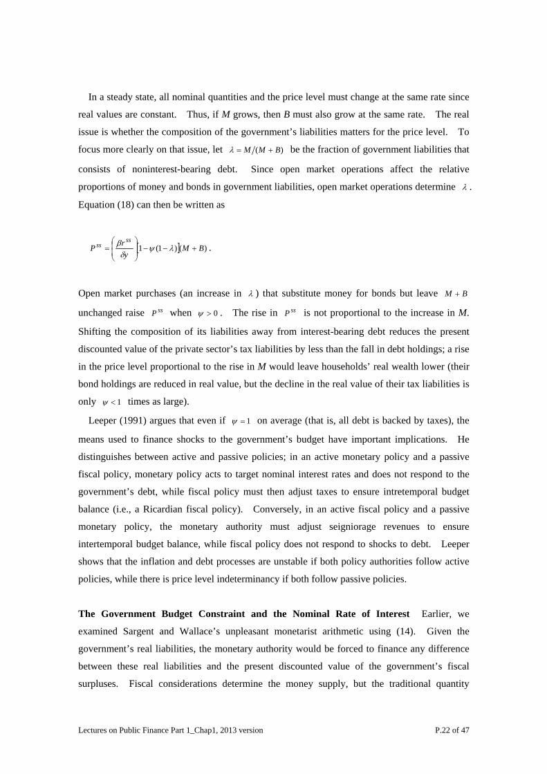
In a steady state, all nominal quantities and the price level must change at the same rate since

real values are constant. Thus, if M grows, then B must also grow at the same rate. The real

issue is whether the composition of the government’s liabilities matters for the price level. To

focus more clearly on that issue, let )( BMM +=λ be the fraction of government liabilities that

consists of noninterest-bearing debt. Since open market operations affect the relative

proportions of money and bonds in government liabilities, open market operations determine λ .

Equation (18) can then be written as

[ ] )()1(1 BM +−−⎟⎟⎠

⎞λψ

yrP

ssss

⎜⎜⎝

⎛=

δβ .

λ ) that substitute money for bonds but leave Open market purchases (an increase in M B+

unchanged raise ssP when ss0>ψ . The rise in P is not proportional to the increase in M.

Shifting the composition of its liabilities away from interest-bearing debt reduces the present

discounted value of the private sector’s tax liabilities by less than the fall in debt holdings; a rise

in the price level proportional to the rise in M would leave households’ real wealth lower (their

bond holdings are reduced in real value, but the decline in the real value of their tax liabilities is

only 1<ψ times as large).

Leeper (1991) argues that even if 1=ψ on average (that is, all debt is backed by taxes), the

means used to finance shocks to the government’s budget have important implications. He

distinguishes between active and passive policies; in an active monetary policy and a passive

fiscal policy, monetary policy acts to target nominal interest rates and does not respond to the

government’s debt, while fiscal policy must then adjust taxes to ensure intretemporal budget

balance (i.e., a Ricardian fiscal policy). Conversely, in an active fiscal policy and a passive

monetary policy, the monetary authority must adjust seigniorage revenues to ensure

intertemporal budget balance, while fiscal policy does not respond to shocks to debt. Leeper

shows that the inflation and debt processes are unstable if both policy authorities follow active

policies, while there is price level indeterminancy if both follow passive policies.

The Government Budget Constraint and the Nominal Rate of Interest Earlier, we

examined Sargent and Wallace’s unpleasant monetarist arithmetic using (14). Given the

government’s real liabilities, the monetary authority would be forced to finance any difference

between these real liabilities and the present discounted value of the government’s fiscal

surpluses. Fiscal considerations determine the money supply, but the traditional quantity


theory holds and the price level is proportional to the nominal quantity of money. Suppose,

however, that the initial nominal stock of money is set exogenously by the monetary authority.

Does this mean that the price level is determined solely by monetary policy, with no effect of

fiscal policy? In fact, the following example illustrates how fiscal policy can affect the initial

equilibrium price level, even when the initial nominal quantity of money is given and the

government’s intertemporal budget constraint must be satisfied at all price levels.

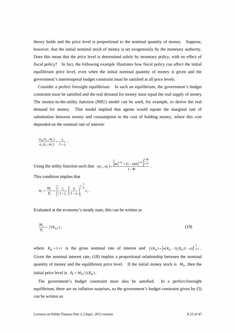
Consider a perfect foresight equilibrium. In such an equilibrium, the government’s budget

constraint must be satisfied and the real demand for money must equal the real supply of money.

The money-in-the-utility function (MIU) model can be used, for example, to derive the real

demand for money. That model implied that agents would equate the marginal rate of

substitution between money and consumption to the cost of holding money, where this cost

depended on the nominal rate of interest:

t

t

ttc

ttmi

imcumcu

+=

1),(),(

[ ]

.

Using the utility function such that Φ

−Φ−

−) 11

1 bbtma

−−+

=−

11(

),(1 bt

ttac

mcu .

This condition implies that

tb

t

t ca

ai

i1

11

−

⎥⎥⎦

⎤

⎢⎢⎣

⎡⎟⎠⎞

⎜⎝⎛

−⎟⎟⎠

⎞⎜⎜⎝

⎛+

t

tt P

Mm == .

Evaluated at the economy’s steady state, this can be written as

)( ,tmt

t RfP

M=

iRm +=1

, (19)

where is the gross nominal rate of interest and [ ] caRR bmm1

)1()1 −−−

0M

aRf m ()( = .

Given the nominal interest rate, (18) implies a proportional relationship between the nominal

quantity of money and the equilibrium price level. If the initial money stock is , then the

initial price level is )(00 mRfMP = .

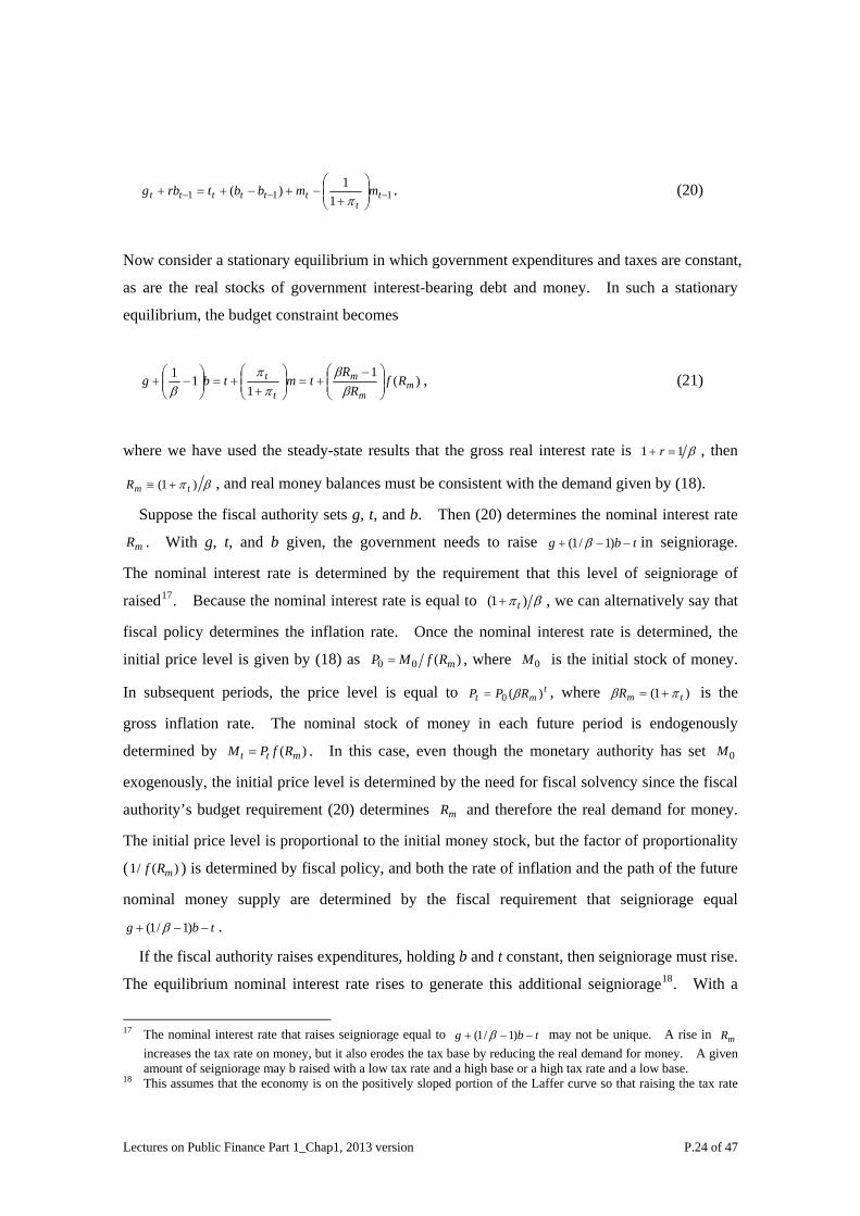
The government’s budget constraint must also be satisfied. In a perfect-foresight

equilibrium, there are no inflation surprises, so the government’s budget constraint given by (5)

can be written as


11 11) −⎟⎟

⎠

⎞⎜⎜⎝

⎛+

−+ tt

t mmπ1 ( −− −+=+ ttttt bbtrbg . (20)

Now consider a stationary equilibrium in which government expenditures and taxes are constant,

as are the real stocks of government interest-bearing debt and money. In such a stationary

equilibrium, the budget constraint becomes

)(1

mm

m RfR

Rt ⎟⎟

⎠

⎞⎜⎜⎝

⎛ −+

ββ

111

t

t mtbg =⎟⎟⎠

⎞⎜⎜⎝

⎛+

+=⎟⎟⎠

⎞⎜⎜⎝

⎛−+

ππ

β, (21)

where we have used the steady-state results that the gross real interest rate is , then β11 =+ r

βπ )1( tm +≡

mR t−

R , and real money balances must be consistent with the demand given by (18).

Suppose the fiscal authority sets g, t, and b. Then (20) determines the nominal interest rate

. With g, t, and b given, the government needs to raise bg −+ )1/1( β in seigniorage.

The nominal interest rate is determined by the requirement that this level of seigniorage of

raised17. Because the nominal interest rate is equal to β1( π )t+ , we can alternatively say that

fiscal policy determines the inflation rate. Once the nominal interest rate is determined, the

initial price level is given by (18) as )(00 mRfMP = , where is the initial stock of money.

In subsequent periods, the price level is equal to , where is the

gross inflation rate. The nominal stock of money in each future period is endogenously

determined by . In this case, even though the monetary authority has set

exogenously, the initial price level is determined by the need for fiscal solvency since the fiscal

authority’s budget requirement (20) determines and therefore the real demand for money.

The initial price level is proportional to the initial money stock, but the factor of proportionality

(1 ) is determined by fiscal policy, and both the rate of inflation and the path of the future

nominal money supply are determined by the fiscal requirement that seigniorage equal

0M

tmt RPP )(0 β= )1( tmR πβ +=

tt fP= 0M

mR

/

)( mRM

(Rf

t−/1(

)m

b− )1g + β .

If the fiscal authority raises expenditures, holding b and t constant, then seigniorage must rise.

The equilibrium nominal interest rate rises to generate this additional seigniorage18. With a

tbg −−+ )1/1( β mR17 The nominal interest rate that raises seigniorage equal to may not be unique. A rise in

increases the tax rate on money, but it also erodes the tax base by reducing the real demand for money. A given amount of seigniorage may b raised with a low tax rate and a high base or a high tax rate and a low base.

18 This assumes that the economy is on the positively sloped portion of the Laffer curve so that raising the tax rate


higher , the real demand for money falls, and this increases the equilibrium value of the

initial price level , even though the initial nominal quantity of money is unchanged.

mR

0P

1.5 The Fiscal Theory of the Price Level

Recently, a number of researchers have examined models in which fiscal factors replace the

money supply as the key determinant of the price level (see Leeper 1991; Sims 1994; Woodford

1995, 1998b, 2001; Bohn 1998b; Cochrane 1998a; Kocherlakota and Phelen 1999; Daniel 2001,

the excellent discussions by Carlstrom and Fuerst 1999b and by Christiano and Fitzgerald 2000,

and references they list, and the criticisms of the approach by McCallum 2001 and Buiter 2002).

The fiscal theory of the price level raises some important issues for both monetary theory and

monetary policy.

There are two ways fiscal policy might matter for the price level. First, equilibrium requires

that the real quantity of money equal the real demand for money. If fiscal variables affect the

real demand for money, the equilibrium price level will also depend on fiscal factors. This

however, is not the channel emphasized in fiscal theories of the price level. Instead, these

theories focus on a second aspect of monetary models – there may be multiple price levels

consistent with a given nominal quantity of money and equality between money supply and

money demand. Fiscal policy may then determine which of these is the equilibrium price level.

And in some cases, the equilibrium price level picked out by fiscal factors may be independent

of the nominal supply of money.

In contrast to the standard monetary theories of the price level, the fiscal theory assumes that

the government’s intertemporal budget equation represents an equilibrium condition rather than

a constraint that must hold for all price levels. At some price levels, the intertemporal budget

constraint would be violated. Such price levels are not consistent with equilibrium. Given

the stock of nominal debt, the equilibrium price level must ensure that the government’s

intertemporal budget is balanced.

The next subsection illustrates why the requirement that the real demand for money equal the

real supply of money may not be sufficient to uniquely determine the equilibrium price level,

even for a fixed nominal money supply. The subsequent subsection shows how fiscal

considerations may serve to pin down the equilibrium price level.

Multiple Equilibria The tradition quantity theory of money highlights the role the nominal

increases revenue.


stock of money plays in determining the equilibrium price level. Using the demand for money

given by (18), we obtained a proportional relationship between the nominal quantity of money

and the equilibrium price level that depended on the nominal rate of interest. However, the

nominal interest rate is also an endogenous variable, so (18) by itself may not be sufficient to

determine the equilibrium price level. Because the nominal interest rate depends on the rate of

inflation, (18) can be written as

⎟⎟⎠

⎞⎜⎜⎝

⎛= +

t

tt

t

tP

PRf

PM 1

0M

,

where R is the gross real rate of interest. As we saw in section 1.3, this forward difference

equation in the price level may be insufficient to determine a unique equilibrium path for the

price level.

Consider a perfect-foresight equilibrium with a constant nominal supply of money, .

Suppose the real rate of return is equal to its steady-state value of β/1 , and the demand for real

money balances is given by (18). We can then write the equilibrium between the real supply

of money and the real demand for money as

0' ,10 <⎟⎟⎠

⎞⎜⎜⎝

⎛= + g

PP

gt

t

t

)(

PM .

Under suitable regularity conditions on •g , this condition can be rewritten as

)(01t

tt P

PM

gP φ≡⎟⎟⎠

⎞⎜⎜⎝

⎛= −

*PP it =+

i )1(0* gMP =

*P≠

1tP + . (22)

Equation (21) defines a difference equation in the price level. One solution is for all

, where . In this equilibrium, the quantity theory holds, and the price level is

proportional to the money supply.

0≥

This constant price level equilibrium is not, however, the only possible equilibrium. As we

saw in section 1.3, there may be equilibrium price paths starting from that are fully

consistent with the equilibrium condition (21). For example, in Figure 1, the convex curve

shows

0P

)( tPφ as an increasing function of . Also shown in Figure 1 is the line. tP o45


Using the fact that , the slope of 1)/ *0 =P(1− Mg )( tPφ , evaluated at *P , is

/)](/(/

(/)/(

0*

0

*0

1

∂

∂−

MPM

MPMg

)/([1

[)/()('*

01

*0

1*

∂−=

∂−=−

−

PMg

PMgPφ

1)

)/)](/*

*0

*0

>P

PMP

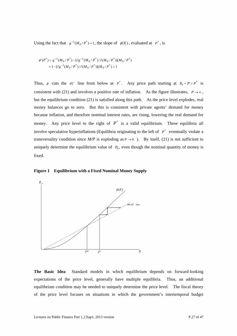
Thus, φ cuts the line from below at o45 *P . Any price path starting at is

consistent with (21) and involves a positive rate of inflation. As the figure illustrates,

*0 ' PPP >=

∞→P

*

,

but the equilibrium condition (21) is satisfied along this path. As the price level explodes, real

money balances go to zero. But this is consistent with private agents’ demand for money

because inflation, and therefore nominal interest rates, are rising, lowering the real demand for

money. Any price level to the right of P is a valid equilibrium. These equilibria all

involve speculative hyperinflations (Equilibria originating to the left of *P eventually violate a

transversality condition since M/P is exploding as ). By itself, (21) is not sufficient to

uniquely determine the equilibrium value of , even though the nominal quantity of money is

fixed.

0→P

0P

Figure 1 Equilibrium with a Fixed Nominal Money Supply

1+tP

P’P*

)( tPφ

tP

the 45°line

The Basic Idea Standard models in which equilibrium depends on forward-looking

expectations of the price level, generally have multiple equilibria. Thus, an additional

equilibrium condition may be needed to uniquely determine the price level. The fiscal theory

of the price level focuses on situations in which the government’s intertemporal budget


constraint may supply the additional equilibrium condition.

The fiscal theory can be illustrated in the context of a model with a representative household

and a government, but with no capital. The implications of the fiscal theory will be earliest to

see if attention is restricted to perfect-foresight equilibria.

The representative household chooses its consumption and asset holdings optimally, subject

to an intertemporal budget constraint. Suppose the period t budget constraint of the

representative household takes the form

dt

t

dt

tD

iM

i 111

+⎟⎟⎠

⎞⎜⎜⎝

⎛+

+⎟⎟⎠

⎞

tD dt

dtt

dt MBiD ++=+ )1(1

d

ttt

dt

dttttttt

icPBMcPTyPD

1⎜⎜⎝

⎛+

+=++≥−+ ,

where is the household’s beginning-of-period financial wealth and .

The superscripts denote that dM and B are the household’s demand for money and

interest-bearing debt. In real terms, this budget constraint becomes

dt

t

dt

t

t dr

mi 11

1+⎟⎟

⎠

⎞⎜⎜⎝

⎛+

+⎟⎟⎠

⎞

(=tr ttt PDd /=

tdt

dttttt

icbmcyd

1⎜⎜⎝

⎛+

+=++≥−+ τ ,

where , and . Let )1)(1 1+++ tti π1,/,/ +== tdt

dtttt PMmPTτ

∏= +

+ ⎟⎟⎠

⎞⎜⎜⎝

⎛

+=

i

j jtitt r

1, 1

1λ

1, =ttλ

be the discount factor, with . Under standard assumptions, the household intertemporal

budget constraint takes the form

⎥⎥⎦

⎤

⎢⎢⎣

⎡⎟⎟⎠

⎞⎜⎜⎝

⎛+

+ ++

++

dit

it

itit m

ii

c1

=−+∞

=+

∞

=+++ ∑∑

iitt

iittittt yd )(

0,

01, λτλ . (23)

Household choices must satisfy this intertemporal budget constraint. The left side is the

present discounted value of the household’s initial real financial wealth and after tax income.

The right side is the present discounted value of consumption spending plus the real cost of

holding money. This condition holds with equality because any path of consumption and

money holdings for which the left side exceeded the right side would not be optimal; the


household could increase its consumption at time t without reducing consumption or money

holdings at any other date. As long as the household is unable to accumulate debts that exceed

the present value of its resources, the right side cannot exceed the left side.

The budget constraint for the government sector, in nominal terms, takes the form

tttt BMMT +−+= −1

tP

tttt BigP ++ −− 11)1( . (24)

Dividing by , this can be written as

111

+⎟⎟⎠

⎞⎜⎜⎝

⎛+

+⎟⎟⎠

⎞+ t

tt

t

t dr

mi

i

itd +

1⎜⎜⎝

⎛+=+ ttt dg τ .

Recursively substituting for future values of , this budget constraint implies that

TTttTit ds +∞→

+ =− ,lim] λi

ittittt gd∞

=+++∑ −+

01, [ τλ , (25)

where )1/( tttt imis +=

tP

is the government’s real seigniorage revenue. In previous sections, we

assumed that the expenditures, taxes and seigniorage choices of the consolidated government

(the combined monetary and fiscal authorities) were constrained by the requirement that

for all price levels . Policy paths for 0, =+∞→ TTttT dλlim such that 0),,,( ≥++++ iitititit dsg τ

0lim] , == +∞→TTttT

i dλ

itp + 0≥i

[0

1, −−+∞

=++++∑

itittittt sgd τλ

for all price paths , are called Ricardian policies. Policy paths for

0) ≥ii, +ti d,, +++ titit sg( τ for which may not equal zero for all price paths are called

non-Ricardian

TTttT d+→∞ ,lim λ

19.

Now consider a perfect-foresight equilibrium. Regardless of whether the government

follows a Ricardian or a non-Ricardian policy, equilibrium in the goods market in this simple

19 Notice that this usage differs somewhat from the way Sargent (1982) and Aiyagari and Gertler (1985) employed the terms. In these earlier papers, a Ricardian policy was one in which the fiscal authority fully adjusted taxes to ensure intertemporal budget balance for all price paths. A non-Ricardian policy was a policy in which the monetary authority was required to adjust seigniorage to ensure intertemporal budget balance for all price paths. Both of these policies would be labeled Ricardian under the current usage of the term.


economy with no capital requires that tt gcty += . The demand for money must also equal the

supply of money: . Substituting tm tgdtm = ty − for and for in (22) and

rearranging yields

tc tm dtm

01 +

+

++ =

⎥⎥⎦

⎤⎟⎟⎠

⎞⎜⎜⎝

⎛+

− itit

iti m

ii

d

01,∑

∞

=++

⎢⎢⎣

⎡−+

ittittt gd τλ . (26)

Thus, an implication of the representative household’s optimization problem and market

equilibrium is that (25) must hold in equilibrium. Under Ricardian policies, (25) does not

impose any additional restrictions on equilibrium since the policy variables are always adjusted

to ensure that this condition holds. Under a non-Ricardian policy, however, it does impose an

additional condition that must be satisfied in equilibrium. To see what this condition involves,

we can use the definition of t and seigniorage to write (25) as

∑∞

=

=0it

tPD

++++ −+ 1, ][ titititt gsτλ

tD

. (27)

At time t, the government’s outstanding nominal liabilities are predetermined by past

policies. Given the present discounted value of the government’s future surpluses (the right

side (26)), the only endogenous variable is the current price level . The price level must

adjust to ensure that (26) is satisfied.

tP

Equation (26) is an equilibrium condition under non-Ricardian policies, but it is not the only

equilibrium condition. It is still the case that real money demand and real money supply must

be equal. Suppose the real demand for money is given by (18), rewritten here as

).1( tt

t ifP

M+=

itg +

it+

(28)

Equation (26) and (27) must both be satisfied in equilibrium. However, which two variables

are determined jointly by these two equations depends on the assumptions that are made about

fiscal and monetary policies. For example, suppose the fiscal authority determines and

τ for all , and the monetary authority pegs the nominal rate of interest =+iti0≥i ι for all

. Seigniorage is equal to 0≥i )1/()1( ιιι ++f and so is fixed by monetary policy. With this


specification of monetary and fiscal policies, the right side of (26) is given. Since is

predetermined at date t, (26) can solved for the equilibrium price level given by

tD

*tP

][, ititititt

t

gsD

++++ −+τλ0

*

itP

∞=Σ

= . (29)

The current nominal money supply is then determined by (27):

)1(* ι+= fPM tt

g

.

One property of this equilibrium is that changes in fiscal policy ( or τ ) directly alter the

equilibrium price level, even though seigniorage as measured by i

*tP

titti s ++∞=Σ ,0λ is unaffected20.

The finding that the price level is uniquely determined by (28) contrasts with a standard

conclusion that the price level is indeterminate under a nominal interest rate peg. This

conclusion is obtained from (27): with i pegged, the right side of (27) is fixed, but this only

determines the real supply of money. Any price level is consistent with equilibrium, as M then

adjusts to ensure that (27) holds.

Critical to the fiscal theory is the assumption that (26), the government’s intertemporal

budget constraint, is an equilibrium condition that holds at the equilibrium price level and not a

condition that must hold at all price levels. This means that at price levels not equal to , the

government is planning to run surpluses (including seigniorage) whose real value, in present

discounted terms, is not equal to the government’s outstanding real liabilities. The government

does not need to ensure that (26) holds for all price levels. Similarly, it means that the

government could cut current taxes, leaving current and future government expenditures and

seigniorage unchanged, and not simultaneously plan to raise future taxes. When (26)is

interpreted as a budget constraint that must be satisfied for all price levels, then any decision to

cut taxes today (and so lower the right side of (26)) must be accompanied by planned future tax

increases to leave the right side unchanged.

In standard infinite-horizon, representative-agent models, a tax cut (current and future

government expenditures unchanged) has no effect on equilibrium (i.e., Ricardian equivalence

holds) because the tax reduction does not have a real wealth effect on private agents. They

20 A change in g or τ causes the price level to jump, and this transfers resources between the private sector and

the government. This transfer can also be viewed as a form of seigniorage.


recognize that in a Ricardian regime, future taxes have risen in present value terms by an

amount exactly equal to the reduction in current taxes. Alternatively expressed, the

government cannot engineer a permanent tax cut unless government expenditures are also cut

(in present value terms). Because the fiscal theory of the price level assumes that (26) holds

only when evaluated at the equilibrium price level, the government can plan a permanent tax cut.

If it does, the price level must rise to ensure that the new, lower value of discounted surpluses is

again equal to the real value of government debt.

An interest rate peg is just one possible policy specification. As an alternative, suppose as

before that the fiscal authority sets the paths for and itg + it+τ , but now suppose that the

government adjusts tax revenues to offset any variations in seigniorage. In this case, itit s ++ +τ

becomes an exogenous process. Then (26) can be solved for the equilibrium price

level ,independent of the nominal money stock. Equation (27) must still hold in equilibrium.

If the monetary authority sets , this equation determines the nominal interest rate that

ensures that the real demand for money is equal to the real supply. If the monetary authority

sets the nominal rate of interest, (27) determines the nominal money supply. The extreme

implication of the fiscal theory (relative to traditional quantity theory results) is perhaps most

stark when the monetary authority fixes the nominal supply of money:

tM

MM it ++ 0≥i for all .

Then, under a fiscal policy that makes its +it+ +τ an exogenous process, the price level is

proportional to and, for a given level of , is independent of . tD tD M

Empirical Evidence on the Fiscal Theory Under the fiscal theory of the price level, (26)

holds at the equilibrium value of the price level. Under traditional theories of the price level,

(26) holds for all values of the price level. If we only observe equilibrium outcomes, it will be

impossible empirically to distinguish between the two theories. As Sims (1994, p.381) puts it,

“Determinacy of the price level under any policy depends on the public’s beliefs about what the

policy authority would do under conditions that are never observed in equilibrium.”

Canzoneri, Cumby, and Diba (2001) examine VAR evidence on th response of U.S. liabilities

to a positive innovation to the primary surplus. Under a non-Ricardian policy, a positive

innovation to ttt gsτ + − is negatively serially correlated. The authors argue that in a

Ricardian regime, a positive innovation to the current primary surplus will reduce real liabilities.

This can be seen by writing the budget constraint (23) in real terms as

)]([ tttt gsdR −+−= τ . (30) 1td +


Examining U.S. data, they find that the responses are inconsistent with a Ricardian regime.

Increases in the surplus are associated with declines in current and future real liabilities, and the

surplus does not display negative serial correlation.

Cochrane points out the fundamental problem with this test: both (29) and (26) must hold in

equilibrium, so it can be difficult to develop testable restrictions that can distinguish between

the two regimes. The two regimes have different implications only if we can observe

nonequilibrium values of the price level.

Bohn (1998) has examined the U.S. deficit and debt processes and concludes that the primary

surplus responds positively to the debt to GDP ratio. In other words, a rise in the debt to GDP

ratio leads to an increase in the primary surplus. Thus, the surplus does adjust, and Bohn finds

that it responds enough to ensure that the intertemporal budget constraint is satisfied. This is

evidence that the fiscal authority seems to act in a Ricardian fashion.

Finally, there is an older literature that attempted to estimate whether fiscal deficits tended to

lead to faster money growth. Such evidence might be interpreted to imply a Ricardian regime

of fiscal dominance.

1.6 Friedman’s Rule Revisted

The preceding analysis has gone partway toward integrating the choice of inflation with the

general public finance choice of tax rates, and the discussion was motivated by Phelps’s

conclusion that some revenue should be raised from the inflation tax if only distortionary tax

sources are available. However, this conclusion has been questioned by Kimbrough (1986a,

1986b), Faig (1988), Chari, Christiano, and Kehoe (1991, 1996), and Correia and Teles (1996,

1999)21. They show that there are conditions under which Friedman’s rule for the optimal

inflation rate – a zero nominal rate of interest – continues to be optimal even in the absence of

lump-sum taxes. Mulligan and Sala-i-Martin (1997) provide a general discussion of the

conditions necessary for taxing (or not taxing) money.

This recent literature integrates the question of the optimal inflation tax into the general

problem of optimal taxation. By doing so, the analysis can build on findings in the optimal tax

literature that identify situations in which the structure of optimal indirect taxes calls for

different final goods to be taxed at the same rate or for the tax rate on goods that serve as

21 An early example of the use of optimal tax models to study the optimal inflation rate issue is Drazen (1979).

See also Walsh (1984). A recent survey is Chari and Kehoe (1999).


intermediate inputs to be zero (see Diamond and Mirrlees 1971, Atkinson and Stiglitz 1972).

An MIU approach, for example, treats money as a final good; in contrast, a shopping time

model, or a more general model in which money serve to produce transaction services, treats

money as an intermediate input. Thus, it is important to examine what implications these

alternative assumptions about the role of money might have for the optimal tax approach to

inflation determination, and how optimal inflation tax results might depend on particular

restrictions on preferences or on the technology for producing transaction services.

The Basic Ramsey Problem The problem of determining the optimal structure of taxes to

finance a given level of expenditures is called the Ramsey problem, after the classic treatment of

Frank Ramsey (1928). In the representative-agent models we have ben using, the Ramsey

problem involves setting taxes to maximize the utility of the representative agent, subject to the

government’s revenue requirement.

The following static Ramsey problem, based on Mulligan and Sala-i-Martin (1997), can be

used to highlight the key issues. The utility of the representative agent depends on

consumption (c), real money balance (m), and leisure (l):

),,( lmcuu =

mcnf m

.

Agents maximize utility subject to the following budget constraint:

ττ ++≥ )1()(

)(nf ln

, (31)

where is a standard production function, −1 is the supply of labor, c is consumption, =

τ is the consumption tax, )i1/(im +=τ is the tax on money, and m is the household’s holdings

of real money balances. The representative agent picks consumption, money holdings, and

leisure to maximize utility, taking the tax rates as given. Letting λ be the Lagrangian

multiplier on the budget constraint, the first order conditions from the agent’s maximization

problem are

(32) )1(λ τ+=cu

mmu λτ+

'ful

(33)

λ= (34)


From these first order conditions and the budget constraint, the choices of c, m, and l can be

expressed as functions of the two tax rates: ),( mc ττ , ),( mm ττ , and ),( ml ττ .

The government’s problem is to set τ and mτ to maximize the representative agent’s utility,

subject to three types of constraints. First, the government must satisfy its budget constraint;

tax revenues must be sufficient to finance expenditures. This constraint takes the form

, (35) gmc m ≥+τ τ

where g is real government expenditures. These expenditures are taken to be exogenous.

Second, the government is constrained by the fact that consumption, labor supply, and real

money must be consistent with the choices of private agents. That means that (31)-(33)

represent constraints on the government’s choices. Finally, the government is constrained by

the economy’s resource constraint:

. (36) gclf +≥− )1(

The government’s problem is to pick τ and mτ to maximize subject to (31)-(36). ),,( lmc

{ }]),()), gc mm

u

There are two approaches to solving this problem. The first approach, often called the dual

approach, employs the indirect utility function to express utility as a function of taxes. These

tax rates are treated as the government’s control variables, and the optimal values of the tax

rates are found by solving the first order conditions from the government’s optimization

problem. The second approach, called the primal approach, treats quantities as the

government’s controls. The tax rates are found from the representative agent’s first order

conditions to ensure that private agents choose the quantities that solve the government’s

maximization problem. We start with the dual approach. The primal approach will be

employed later in this section.

The government’s problem can be written as

(1([]),(),([),(max,

lfgcmv mmmmm

−−−+−++ τ τττθττττττμττττ

,

where )],(),,(),, mmm lm([),( m cuv ττττττττ is the indirect utility function, and μ and θ are

Lagrangian multipliers on the budget and resource constraints. Notice that we have


incorporated the constraints represented by (31)-(33) by writing consumption, money balances,

and leisure as functions of the tax rates. The first order conditions for the two taxes are

0)'() ≤+( −+++ τ τττττμ θ clfc

0)'()

cmv mt

( +−mm

clf ττ+++mmm

cmmv mt ττ ≤θττμ ,

where τττ lumuc lmcutv ++m

vt=mmm

lumucu lmc τττ and ++= . These conditions will hold with

equality if the solution is an interior one with positive taxes on both consumption and money.

If the left side of the second first order condition is negative optimal. From the resource

constraint (36), 0' =−− xx clf x for mττ ,= since g is fixed, so the two first order conditions can

be simplified to yield

0)( ≤++ τττμ τ+++ τττ ccmm

0)

lumucu lmc (37)

( +++++mmm

lumucu lmc τττ mmcmm m ττ τ ≤τμ . (38)

The first three terms in the first of these equations can be written using the agent’s first order

conditions and the budget constraint as

[ ]τττ ττ lfmc m ') +++ττττττ fu

lmuu

cuu

ulumucu l

l

m

l

cllmc 1(

' ⎟⎟⎠

⎞⎜⎜⎝

⎛=⎟⎟

⎠

⎞⎜⎜⎝

⎛+++++ .

However, differentiating the budget constraint by τ yields

1( ++ 0') =++ ττττ τ lfmc m

cfulum ll )'/(

c ,

so ucu mc −=+ ττ+τ . Thus, (37) becomes

)( ττ ττμ ccmc m ++≥⎟⎟⎠

⎞'f

ul⎜⎜⎝

⎛ ,

while following similar steps implies that (38) becomes


)mτ( mm mτμ +

'm

ful ≥⎟⎟

⎠

⎞⎜⎜⎝

⎛ . m

cτ τ+

Hence, if the solution is an interior one with positive taxes on consumption and money holdings,

ττ

ττ

ττττccmcmm

cm

m

m mm

++

++=

'/ fmulu ll m

. (39)

To interpret this condition, note that mucuv mc mmm=++= −ττττ

'/ fculumucuv llmc

is the effect of the

tax on money on utility, while −=++= ττττ is the effect of the consumption

tax on utility. Thus, their ratio, m/c, is the marginal rate of substitution between the two tax

rates, holding constant the utility of the representative agent22. The right hand side of (39) is

the marginal rate of transformation, holding the government’s revenue constant. At an

optimum, the government equates the marginal rates of substitution and transformation.

Our interest is in determining when the Friedman rule, 0=mτ , is optimal. Assume,

following Friedman, that at a zero nominal interest rate, the demand for money is finite. Since

the tax on consumption must be positive if the tax on money is zero (since the government does

need to raise revenue), (37) will hold with equality. Then

ττ

ττ

ττττccmcmm

cm

m

m mm

++

++≥ . (40)

or

τττ τττ ccmc

c mm++

≥

0=mτ

ττ mmm

m m++ .

The left side is proportional to the marginal impact of the inflation tax on utility per dollar of

revenue raised. The right side is proportional to the marginal impact of the consumption tax

on utility per dollar of revenue raised. If the inequality is strict at , then the distortion

caused by using the inflation tax (per dollar of revenue raised) exceeds the cost of raising that

),( mv ττ

0=+ mdvdvm

22 That is, if is the utility of the representative agent as a function of the two tax rates, then

ττ ττ yields cm

v

v

dd m

m−=−=

τ

τ

ττ .


same revenue with the consumption tax. Thus, it is optimal to set the tax on money equal to

zero if

τ

τ

ττ

cccm

cm m

+

+≥

0≤τc

(41)

or (since )

τcc

0=mτ

0=m

cτ

0>m

cτ

0

τcm m≤ , (42)

where these expressions are evaluated at .

Mulligan and Sala-i-Martin (1997) consider (40) for a variety of special cases that have

appeared in the literature. For example, if utility is separable in consumption and money

holdings, then ; in this case, the right side of (42) is equal to zero, while the left side is

positive. Hence, (42) cannot hold and it is optimal to tax money.

A second case that leads to clear results occurs if . In this case, the right side of (42)

is negative (since <τc

c/ >

0

, an increase in the consumption tax reduces consumption). Because

the left side is nonnegative, m and money should always be taxed. This

corresponds to a case in which money and consumption are substitutes so that an increase in the

tax on money (which reduces money holdings) leads to an increase in consumption. Finally, if

money and consumption are complements,

ττ ccm

/

<mτ ττ c

m/c . The ratio c is then positive, and

whether money is taxed will depend on a comparison of m/c and . τc/τc m

Chari, Christiano, and Kehoe (1996) examine the optimality of the Friedman rule in an MIU

model with taxes on consumption, labor supply, and money. They show htat if preferences are

homothetic in consumption and money balances and separable in leisure, the optimal tax on

money is zero. When preferences satisfy these assumptions, we can write

]),,([),,( lmcsulmcu =

,

where s(c,m) is homethetic23. Mulligan and Sala-i-Martin (1997) show that in this case,

is23 Homethetic preferences imply that s(c,m) is homogeneous of degree 1 and that is homogeneous of degree 0.

With homothetic preferences, indifference curves are parallel to each other, with constant slope along any ray;


τ

τ

cc

cm m=

0=m

111)1( −−− +++ ttt MBi

cτ hτ )(c

)1( l−

,

so (42) implies that the optimal tax structure yields . τ

Chari, Christiano, and Kehoe relate their results to the optimal taxation literature in public

finance. Atkinson and Stiglitz (1972) show that if two goods are produced under conditions of

constant returns to scale, a sufficient condition for uniform tax rates is that the utility function is

homothetic. With equal tax rates, the ratio of marginal utilities equals the ratio of producer

prices. To see how this applies in the present case, suppose the budget constraint for the

representative household takes the form

)1()1()1( −−=+++ tthttttt

ct lQBMcQ ττ ,

where M and B are the nominal money and bond holdings, i is the nominal rate of interest, Q is

the producer price of output, and and are the tax rates on consumption and hours

of work . In addition, we have assumed that the production function exhibits constant

returns to scale and that labor hours, l−1 , are transformed into output according to ly −=1

QP c )1( τ+≡ ttttt mPBM

.

Define . Household real wealth is w tb+= + =/)( , and the budget

constraint can be written as

11

11

111

1)

1)

−−

−

−−−

⎟⎟

⎠

⎞

⎜⎜

⎝

⎛

+−

++

tt

tt

t

ttt

mi

w

mb

π

τ

tτ ≡− 1()1

1()1)(1(

1()1(11

−++−−=

++−⎟⎟⎠

⎞⎜⎜⎝

⎛

+

−=+

ttt

tct

ht

tt

rl

rlwc

τ

ττ

(43)

where and )1/()1( ct

ht ττ +− 1( tr1 )1/()1 tti π++=+ −− 1/ 1 −, and = −ttt PPπ . Thus, the

consumption and labor taxes only matter through the composite tax τ , so without loss of

generality, set the consumption tax equal to zero. If the representative household’s utility

during period t is given by ]),l,([ mcsu and the household’s objective is to maximize

]),, ititi lm ++([ ti csu +β

0itE ∞=∑ subject to the budget constraint given by (43), then the first order

)/(),(/),( 12 cmfmcumcu =


conditions for the household’s decision problem imply that consumption, money balances, and

leisure will be chosen such that

tmt

t

tt

tti

imcmc

,1),(),( τ≡

+=

0, =tmτ

*mm <

*mm ≥

c

m

tttc

tttmss

lmculmcu

),,(),,(= .

With the production costs of money assumed to be zero, the ratio of marginal utilities differs

from the ratio of production costs unless . Hence, with preferences that are homothetic

in c and m, the Atkinson-Stiglitz result implies that it will be optimal to set the nominal rate of

interest equal to zero.

Correia and Teles (1999) consider other cases in which (41) holds so that the optimal tax on

money equals zero. They follow Milton Friedman (1969) in assuming a satiation level of

money holdings m* such that the marginal utility of money is positive for and

nonpositive for . This satiation level can depend on c and l. Correia and Teles show

that the optimal tax on money is zero if ckm =* for a positive constant k

∞=*m

. They also show

that the optimal tax on money is zero if . Intuitively, at an optimum, the marginal

benefit of additional money holdings must balance the cost of the marginal effect on

government revenues. This contrasts with the case of normal goods, where the marginal

benefit must balance the costs of the marginal impact on the government’s revenue and the

marginal resource cost of producing the goods. Money, in contrast, is assumed to be costless

to produce. At the satiation point, the marginal benefit of money is zero. The conditions

studied by Correia and Teles (1999) ensure that the marginal revenue effect is also zero.

We can recover Friedman’s rule for the optimal rate of inflation even in the absence of

lump-sum taxes. But it is important to recognize that the restrictions on preferences necessary

to restore Friedman’s rule are very strong and, as discussed by Braun (1991), different

assumptions about preferences will lead to different conclusions. The assumption that the ratio

of the marginal utilities of consumption and money is independent of leisure can certainly be

questioned. However, it is very common in the literature to assume separability between

leisure, consumption, and money holdings. The standard log utility specification, for example,

displays this property and so would imply that a zero nominal interest rate is optimal.


1.7 Nonindexed Tax Systems

Up to this point, our discussion has assumed that the tax system is indexed so that taxes are

levied on real income; a one-time change in all nominal quantities and the price level would

leave the real equilibrium unchanged. This assumption requires that a pure price change have

no effect on the government’s real tax revenues or the tax rates faced by individuals and firms in

the private sector. Most actual tax systems, however, are not completely indexed to ensure

that pure price-level changes leave real tax rates and real tax revenue unchanged.

Inflation-induced distortions generated by the interaction of inflation and the tax system have

the potential to be much larger than the revenue-related effects on which most of the seigniorage

and optimal inflation literature has focused. Feldstein (1998) provides and analysis of the net

benefits of reducing inflation from 2% to zero24, and he concludes that for his preferred

parameter values, the effects due to reducing distortions related to the tax system are roughly

twice those associated with the change in government revenue.

One important distortion arises when nominal interest income, and not real interest income, is

taxed. After-tax real rates of return will be relevant for individual agents in making savings

and portfolio decisions, and if nominal income is subject to a tax rate of τ , the real after-tax

return will be

τ π τ τ−−=−− ri )1() π=ra 1( ,

where π+= ri is the nominal return and r is the before-tax real return. Thus, for a given

pretax real return r, the after-tax real return is decreasing in the rate of inflation.

To see how this distortion affects the steady-state capital-labor ratio, consider the basic MIU

model with an income tax of τ on total nominal income. Nominal income is assumed to

include any nominal capital gain on capital holdings:

11 /)1)(( −−111)( −−− −− ttt kPP+++≡ ttttttt TPBikfPY δ .

The representative agent’s budget constraint becomes

()1()1( 1− −+−−+=− ttttttt kPkPcPY )() 11 −− + tttt MMBBδτ ,

24 Feldstein allows for an upward bias in the inflation rate, as measured by the consumer price index, so that his

estimates apply to reducing consumer price inflation from 4% to 2%.


where M is the agent’s nominal money holdings, B is his bond holdings, and is a nominal

transfer payment

ttTP

25. In real terms the budget constraint becomes26

.1

11)()1(

111

111

1

⎟⎟⎠

⎞⎜⎜⎝

⎛+

−+⎟⎟⎠

⎞⎜⎜⎝

⎛+

−+−−+=

⎟⎟⎠

⎞⎜⎜⎝

⎛+

−⎥⎦

⎤⎢⎣

⎡+

++−

−−−

−−−

−

t

tt

t

ttttt

tt

tt

t

ttt

mmbbkkc

Tbikf

ππδ

ππ

τπ

τ )1( − kδ

1)1(

Assuming the agent’s objective is to maximize the present discounted value of expected

utility, which depends on consumption and money holdings, the first order conditions for capital

and bonds imply, in the steady state,

βδ

ππτ 1)1(

1)1(

=−⎥⎦⎤

+−+τ 1)()1( ⎢⎣

⎡+− kfk (44)

and

βπτ

πτ 1

111) =

++⎟

⎠⎞

⎜⎝⎛++ i1( − . (45)

The steady-state capita-labor ratio is determined by

⎭⎬⎫

−⎥⎦

⎤⎢⎣

⎡+−+

− )1(1

)1(1δ

ππτ

1/(])1(1[

⎩⎨⎧⎟⎠⎞

⎜⎝⎛

−=

11

1)(βτ

ssk kf .

Because )πτ π +−+ ssk,π

is decreasing in is decreasing in the inflation rate. Higher

inflation leads to larger nominal capital gains on existing holdings of capital, and since these are

taxed, inflation increases the effective tax rate on capital.

Equation (44) can be solved for the steady-state nominal rate of interest to yield

0

25 For simplicity, assume that T is adjusted in a lump-sum fashion to ensure that variations in inflation and the tax rate on income leave the government’s budget balanced. Obviously, if lump-sum taxes actually were available, the optimal policy would involve setting =τ and following Freidman’s rule for the optistate capital stock in the easiest possible manner.

26 This formulation assumes that real economic depreciation is tax deductible. If depreciation allowances are based on historical nominal cost, a further inflation-induced distortion would be introduced.


ττ

τπ

β −−⎟⎠⎞

⎜⎝⎛

−+

=11

11ssi

)1/()1(

+1 .

Thus, the pretax real return on bonds, + +πi

, increases with the rate of inflation, implying

that nominal rates rise more than proportionately with an increase in inflation.

It is important to recognize that we have examined only one aspect of the effects of inflation

and the tax system27. Because of the taxation of nominal returns, higher inflation distorts the

individual’s decisions, but it also generates revenue for the government that, with a constant

level of expenditures (in present value terms), would allow other taxes to be reduced. Thus,

the distortions associated with the higher inflation are potentially offset by the reduction in the

distortions caused by other tax sources. As noted earlier, however, Feldstein (1998) argues

that the offset is only partial, leaving a large net annual cost of positive rates of inflation.

Feldstein identifies the increased effective tax rate on capital that occurs because of the

treatment of depreciation and the increased subsidy on housing associated with the deductibility

of nominal mortgage interest in the United States as important distortions generated by higher

inflation interacting with a nonindexed tax system. Including these effects with an analysis of

the implications for government revenues and, consequently, possible adjustments in other

distortionary taxes, Feldstein estimates that a 2% reduction in inflation (from 2% to zero)

increases net welfare by 0.63% to 1.10% of GDP annually. These figures assume an elasticity

of savings with respect to the after-tax real return of 0.4 and a deadweight loss of taxes of

between 40 cents for every dollar of revenue (leading to the 0.63% figure) and $1.50 per dollar

of revenue (leading to the 1.01% figure). Since these are annual gains, the present discounted

value of permanently reducing inflation to zero would be quite large.

1.8 Summary

Monetary and fiscal actions are linked through the government’s budget constraint. Under

Ricardian regimes, changes in the money strock or its growth rate will require some other

variable in the budget constraint – taxes, expenditures, or borrowing – to adjust. With fiscal

dominance, changes in government taxes or expenditures can require changes in inflation.

Under non-Ricardian regimes, changes in government debt affect prices even if monetary policy

is exogenous. A complete analysis of price level determinacy requires a specification of the

relationship between fiscal and monetary policies.

27 Feldstein, Green, and Sheshinski (1978) used a version of Tobin’s money and growth model (Tobin 1965) to explore the implications of a nonindexed tax system when firms use both debt and equity to finance capital.


Despite this and despite the emphasis budget relationships have received in the work of

Sargent and Wallace and the work on the fiscal theory of the price level initiated by Sims and

Woodford, much of monetary economics ignores the implications of the budget constraint.

This is valid in the presence of lump-sum taxes; any effects on the government’s budget can

simply be offset by an appropriate variation in lump-sum taxes. Traditional analyses that focus

only on the stock of high-powered money are also valid when governments follow a Ricardian

policy of fully backing interest-bearing debt with tax revenues, either now or in the future. In

general, though, we should be concerned with the fiscal implications of any analysis of

monetary policy, since changed in the quantity of money that alter the interest payments of the

government have implications for future tax liabilities.


References Aiyagari, S.R. and M. Gertler (1985) “The Backing of Government Bonds and Monetarism”

Journal of Monetary Economics, 16(1), pp.19-44. Atkinson A.B. and J.E. Stiglitz (1972) “The structure of indirect taxation and economic

efficiency” Journal of Public Economics, 1, pp.97-119. Barro, R.J. (1974) “Are Government bonds Net Wealth?” Journal of Political Economy, 82(6),

Nov./Dec., pp.1095-118. Bohn, H. (1992) “Budget Deficits and Government Accounting.” Carnegie-Rochester

Conference Series on Public Policy, 37, December, pp.1-884. Bohn, H. (1998) “The Behavior of U.S. Public Debt and Deficits.” Quarterly Journal of

Economics, 113 (3), pp.949-64. Braun, R.A. (1991) “Comment on Optimal Fiscal and Monetary Policy: Some Recent Results”

Journal of Money, Credit, and Banking, 23(3), Part 2, Aug., pp.542-546. Buiter, W. (2002) “The Fiscal Theory of the Price Level: A Critique” The Economic Journal,

112(481), July, pp.459-480. Canzonery, M.B., R.E. Cumby, and B.T. Diba (2001) “Is the Price level Determined by the

Needs of Fiscal Solvency?” American Economic Review, 91(5), Dec., pp.1221-1238. Carlstrom, C.T. and T.S. Fuerst (1999b) “The Fiscal Theory of the Price Level” Federal

Reserve Bank of Cleveland, Dec.. Chari, V.V. and P.J. Kehoe (1999) “Optimal Fiscal and Monetary Policy” in J. Taylor and M.

Woodford (eds.), Handbook of Macroeconomics, Vol.1C, Amsterdam: Elsevier North-Holland, pp.1671-1745.

Chari, V.V., L.J. Christiano and P.J. Kehoe (1991) “Optimal Fiscal and Monetary Policy: Some Recent Results” Journal of Money, Credit, and Banking, 23(3), Part 2, Aug., pp.519-39.

Chari, V.V., L.J. Christiano and P.J. Kehoe (1996) “Optimality of the Friedman Rule in Economics with Distorting Taxes” Journal of Monetary Economics, 37(2), Apr., pp.203-23.

Christiano, L.J. and T.J. Fitzgerald (2000) “Understanding the Fiscal Theory of the Price Level” NBER Working Paper No.7668, Apr.

Cochrane, J.H. (1998a) “A Frictionless View of U.S. Inflation” NBER Macroeconomics Annual, Cambridge, MA: MIT Press, pp.323-84.

Correia, I. and P. Teles (1996) “Is the Friedman Rule Optimal When Money Is an Intermediate Good?” Journal of Monetary Economics, 38(2), Oct., pp.223-44.

Correia, I. and P. Teles (1999) “The Optimal Inflation Tax” Review of Economic Dynamics, 2, pp.325-46.

Daniel, B. (2001) “The Fiscal Theory of the Price Level in an Open Economy” Journal of Monetary Economics, 48(2), Oct., pp.293-308.

Demopoulos, G.D., G.M. Katsimbris, and S.M. Miller (1987) “Monetary Policy and Central-Bank Financing of Governemnt Budget Deficits” European Economic Review, 31(5), July, pp.1023-50.

Diamond, P.A. and J.A. Mirrlees (1971) “Optimal taxation and public production I: production efficiency and II: tax rules” American Economic Review, 61, 8-27 and 261-78.

Drazen, A. (1979) “The Optimal Rate of Inflation Revisited” Journal of Monetary Economics, 5(2), April, pp.231-48.

Faig, M. (1988) “Characterization of the Optimal Tax on Money When It Functions as a Medium of Exchange” Journal of Monetary Economics, 22(1), July, pp.137-48.

Feldstein M. (1998) “The Costs and Benefits of Going from Low Inflation to Price Stability” in C. Romer and D. Romer (eds.), Monetary Policy and Inflation, Chicago: University of Chicago Press, pp.123-156.

Feldstein M., J. Green and E. Sheshinski (1978) “Inflation and Taxes in a Growing Economy with Debt and Equity Finance” Journal of Political Economy, 86(2), part 2, April, S53-S70.


Friedman, M. (1969) “The Optimum Quantity of Money” in his The Optimum Quantity of Money and Other Essays, Chicago: Aldine.

Grier, K.B. and H.E. Neiman (1987) “Deficits, Politics and Money Growth” Economic Inquiry, 25(2), Apr. pp.201-14.

Joines, D.H. (1985) “Deficits and Money Growth in the United States 1872-1983” Journal of Monetary Economics, 16(3), Nov. pp.329-51.

Kimbrough, K.P. (1986a) “Inflation, Employment, and Welfare in the Presence of Transaction Costs” Journal of Money, Credit and Banking, 28(2), May, pp.127-40.

Kimbrough, K.P. (1986b) “The Optimum Quantity of Money Rule in the Theory of Public Finance” Journal of Monetary Economics, 18(3), Nov. pp.277-84

King, R.G., and C.I. Plosser (1985) “Money, Deficits, and Inflation.” Carnegie-Rochester Conference Series on Public Policy, 22, Spring, pp.147-96.

Klein, M., and M.J. Neumann (1990) “Seigniorage: What Is It and Who Gets It?” Weltwirt-schaftliches Archiv, 126 (2): 205-21.

Kocherlakota, N.R. and C. Phelen, (1999) “Explaining the Fiscal Theory of the Price Level” Federal Reserve Bank of Minneapolis Quarterly Review, Fall, pp.14-23.

Leeper, E.M. (1991) “Equilibria Under ‘Active’ and ‘Passive’ Monetary and Fiscal Policies” Journal of Monetary Economics, 27 (1), Feb., pp.129-47.

McCallum, B.T. (2001) “Indeterminacy, Bubbles and the Fiscal Theory of Price Level Determination” Journal of Monetary Economics, 47(1), Feb., pp.19-30.

Meltzer, L. (1951) “Wealth, Saving, and the Rate of Interest” Journal of Political Economy, 59(2), Apr., pp.93-116.

Mulligan, C.B. and X. Sala-i-Martin (1997) “The Optimum Quantity of Money: Theory and Evidence” Journal of Money, Credit, and Banking, 24(4), Part 2, Nov., pp.687-715.

Patinkin, D. (1965) Money, Interest, and Prices: An Integration of Monetary and Value Theory, 2nd ed., New York: Harper & Row.

Ramsey, F.P. (1928) “A Mathematical Theory of Saving” Economic Journal, 38(152), Dec., pp.543-59.

Romer, D.H. (2001) Advanced Macroeconomics, New York: McGraw-Hill, 2nd ed. Sargent, T.J. (1982) “Beyond Supply and Demand Curves in Macroeconomics” American

Economic Review, 72(2), May, pp.382-9. Sargent, T.J. (1987) Dynamic Macroeconomic Theory. Cambridge, MA: Harvard University

Press. Sargent, T.J., and N. Wallace (1981) “Some Unpleasant Monetarist Arithmetic.” Federal

Reserve Bank of Minneapolis, Quarterly Review, 5, no.3, 1-17. Sims, C.A. (1994) “A Simple Model for Study of the Determination of the Price Level and the

Interaction of Monetary and Fiscal Policy” Economic Theory, 4, pp.381-99. Tobin, J. (1965) “Monetary and Economic Growth” Econometrica, 33(4), Part 2, Oct.,

pp.671-84. Wallace, N. (1981) “A Modigliani-Miller Theorem for Open-Market Operations” American

Economic Review, 71, no.3 (June): 267-74. Walsh, C.E. (1984) “Optimal Taxation by the Monetary Authority” NBER Working Paper

No.1375, June. Walsh, Carl E. (1998) Monetary Theory and Policy, 2nd ed., The MIT Press. Woodford, M. (1995) “Price Level Determinacy without Control of a Monetary Aggregate.”

Carnegie-Rochester Conference Series on Public Policy, 43, pp.1-46. Woodford, M. (1995) “Price Level Determinacy without Control of a Monetary Aggregate”

Carnegie-Rochester Conference Series on Public Policy, 43, Dec, pp.1-46. Woodford, M. (1998b) “Comment: A Frictionless View of U.S. Inflation” NBER

Macroeconomics Annual, Cambridge, MA: MIT Press, pp.390-419. Woodford, M. (2001a) “Inflation Stabilization and Welfare” NBER Working Paper, No.8071,

Jan.



Woodford, M. (2001b) “Fiscal Requirements for Price Stability?” Journal of Money, Credit and Banking, 33(3), Aug. pp.669-728.

Woodford, M. (2003) Interest and Prices: Foundations of a Theory of Monetary Policy, Princeton University Press.

Documents

Chapter 1 Monetary and Fiscal Policy1 - Keio and... · Chapter 1 Monetary and Fiscal Policy. 1. 1.1 Introduction. A public-finance approach yields several insights. Among the most