Chapter 1: Modelling the movement and spatial distribution

Humpback whale use of the Kimberley: understanding and monitoring spatial distribution

Kimberley Marine Rsearch Program Project 1.2.1 1

Chapter 1: Modelling the movement and spatial distribution of humpback whales in the nearshore waters of the Kimberley

Michele Thums1,4, Curt Jenner2,4, Vinay Udyawer1,4, Luciana Ferreira1,4, Kelly Waples3,4, Micheline Jenner2,4, Mark

Meekan1,4 1Australian Institute of Marine Science, Perth, Western Australia, Australia 2Centre for Whale Research, Perth, Western Australia, Australian Institute of Marine Science 3Western Australia Department of Biodiversity, Conservation and Attractions, Perth, Western Australia, Australia 4Western Australian Marine Science Institution (WAMSI), Perth, Western Australia, Australia

1 Introduction

One of the key steps to achieving visible, tangible and significant conservation benefits for the marine

biodiversity of the Kimberley is to gain an understanding of how megafauna use the region. This information

can enable managers to determine if and how patterns of use change over time in response to natural or

anthropogenic pressures. The knowledge required for this process includes relative abundance, distribution,

movement patterns (travelling, resting, etc.) and habitat use, along with the environmental context of these

patterns. This information is fundamental to the delivery of appropriate management strategies at both single

species and ecosystem scales.

Off the west coast of Australia, a population of 33,000 humpback whales (at minimum) migrate annually from

summer feeding grounds in Antarctica to breed and calve during winter in the nearshore waters of the

Kimberley (Salgado-Kent et al. 2012). This population was decimated during the whaling era, but is recovering

strongly at an estimated rate of over 11% per annum (Salgado-Kent et al. 2012). Within the Kimberley region,

Camden Sound has been identified as a key area for calving, with other important areas of aggregation

including Pender Bay and the area surrounding Frost and Tasmanian shoals (Jenner et al. 2001).

Since the recognition of the nearshore waters of the Kimberley as a calving ground in the mid 1990’s (Jenner et

al. 2001), there have been many boat-based and aerial surveys of humpback whales in the region conducted by

industry, researchers and others, along with complementary studies using satellite tagging to determine

abundance, distribution and movement patterns of this population. However, much of the data remain

unpublished and there has been no synthesis of this data in order to provide a broad understanding of how

humpback whales use the Kimberley, particularly as a breeding area. Such information is vital for both the

management of human activities, including the emerging tourism industry of whale watching in breeding

grounds in Lalang garram/Camden Sound Marine Park, as well as the documentation of expansion or

movement from this area as a result of population growth and increasing anthropogenic activities in the

Kimberley region.

The purpose of our project was to compile and analyse existing survey and tracking data of humpback whales

to build a clear picture of the distribution, absolute abundance, movements and habitat use (in particular

calving areas) by the species through the Kimberley region and to identify the environmental factors that are

associated with these patterns. Additionally, we set out to identify information gaps and provide advice for

future monitoring and management (Chapter 4) by assessing a range of methods including high resolution

satellite imagery for detecting and counting whales (Chapter 2), aerial and boat based surveys and the use of a

land based platform at Pender Bay (Chapter 3).


2 Kimberley Marine Research Program | Project 1.2.1

2 Materials and Methods

Historical survey data of humpback whales were compiled from the Kimberley region of Western Australia

(Table 1). These included dedicated (researchers and consultants on behalf of oil and gas companies) and non-

dedicated (e.g. tourist operators and Customs surveillance) surveys from vessels and aircraft. These surveys

usually took place between July and October and in addition to counting humpback whales, many surveys also

recorded sightings of a range of other marine megafauna (e.g. dugongs, marine turtles, etc.). In some cases, the

survey coverage was designed to address specific issues of an industry client that commissioned the research

and was not necessarily related to the estimation of abundance and distribution of humpback whales

throughout their range in the Kimberley region (e.g. RPS Group/Woodside surveys focussed at James Price

Point, Table 1). Each dataset was assessed to determine the appropriate modelling method to be used for

analysis. Where a dataset was collected with distance sampling methods (Buckland et al. 2011) and survey

paths were available to calculate effort, we used density surface modelling to analyse the observation data (as

counts). Where this was not possible, or where sampling effort was spatially restricted (as mentioned above)

we used the Maximum Entropy Method (MaxEnt), a species distribution modelling approach, to model

observations as presence/absence data (Table 1). Some datasets were deemed unusable for either analysis

(Table 1).

Dedicated surveys included both vessel-based and aerial line transects conducted in both zigzag patterns and

parallel lines perpendicular to coast over the study area which sometimes differed in structure in each year.

Tracking data from satellite tags that was collected over three years (2008, 2009 and 2011) was also analysed

to provide details of the movement behaviour of whales of known sex and breeding status (cows with calves)

to determine areas with highest residence and to document the area of use on each of the northward and

southward migrations.

The spatial extent of the modelling was determined by the spatial extent of the surveys and although we refer

to ‘the Kimberley’ throughout this report, it technically refers to the area of the Kimberley surveyed (Fig. 1).

Table 1. Aerial and vessel line transect survey data compiled for the project and the response variable used for modelling.

Species distribution modelling (using MaxEnt) was used for presence/absence data and density surface modelling used for

counts, RPS = RPS Group, environmental consultants.

Platform

Year Sample days Total whales

Survey program Months covered Response

variable

Aerial 1993 75 805 Coastwatch/CWR Jun, Jul, Aug, Sept presence/absence

Aerial 2006 4 279 CWR Aug, Sept counts

Aerial 2007 7 1050 CWR Aug, Sept counts

Aerial 2008 9 1979 CWR Jul, Aug, Sept, Oct counts

Aerial 2008 7 172 CWR Aug, Sept, Oct presence/absence

Aerial 2009 9 568 RPS/Woodside Jul, Aug, Sept, Oct presence/absence



Aerial 2009 8 962 RPS/Woodside Jul, Aug, Sept presence/absence

Aerial

2010 10 530

RPS/Woodside Jun, Jul, Aug, Sep,

Oct

presence/absence

Aerial 2010 10 377 RPS/Woodside Jun, Jul, Aug, Sep, presence/absence



Oct

Aerial 2011 7 490 RPS/Woodside Jun, Jul, Aug, Sep presence/absence

Aerial 2012 7 762 RPS/Woodside Jul, Aug, Sep, Oct presence/absence

Boat

based 1995 39 372

CWR Aug, Sept, Oct presence/absence

Boat

based 1996 52 667

CWR Jul, Aug, Sept, Oct presence/absence

Boat

based 1997 58 904

CWR Jul, Aug, Sept presence/absence

Boat

based 2006 70 534

CWR/Inpex Aug, Sept presence/absence

Boat

based 2007 27 461

CWR/Inpex Jul, Aug presence/absence

Boat

based 2008 58 57

CWR/Inpex Jun, Jul, Oct, Nov presence/absence

Boat

based 2008 13 401

CWR/Woodside Sept, Oct presence/absence

Boat

based 2009 25 1262

RPS/Woodside Jul, Aug, Sept, Oct presence/absence

Boat

based 2008 6 131

WAMSI Sep *

Boat

based 2009 6 380

WAMSI Aug, Sep *

Boat

based 2010 3 86

WAMSI Aug *

Boat

based 2011 8 498

WAMSI Aug *

Boat

based 2010 27 1155

Costin (tourist

operator)

Jun, July, Aug, Sep presence/absence

Boat

based 2011 13 907

Costin (tourist

operator)

Jul, Aug presence/absence

Boat

based 2013 14 893

Costin (tourist

operator)

Aug, Sep presence/absence

Boat

based 2014 6 332

Costin (tourist

operator)

Sep presence/absence

total 691 18031

* The positions recorded in the data are boat positions, not whale positions and distance and bearing were not recorded

thus, whale positions could not be calculated.



2.1 Dedicated surveys

Aerial surveys

Aerial surveys by CWR (Jenner & Jenner 2007a, b, 2009) were conducted at an altitude of 305 m (1000 ft) and a

speed of 222 km/hr (120 knots) using a twin-engine, over-head wing aircraft (Twin Otter or Cessna 337). The

plane followed zigzag transects that operated in passing mode (i.e. the plane did not deviate from the flight

path). Surveys were only initiated in wind speeds < 33 km h-1 (18 knots), which has been shown to be adequate

for spotting whales (Salgado-Kent et al. 2012). Each flight was of approximately 5.5 to 6 hours duration and

take-off times varied between 8:40 and 10:55 so that the mid-day period was always sampled and glare would

be a consistent factor for all flights. Personnel for each survey included two pilots and two observers. The pilots

were responsible for recording the angle of drift of the plane on each transect, so that angles of whale sightings

reported from the compass boards (see below) could be corrected relative to the flight path (Lerczac & Hobbs

2006). The observers were linked via a separate intercom system that was logged to a Sony Mini Disk Recorder

NH900, allowing the observers to search continuously and voice record all sightings to a time code that was

synchronized to the Global Positioning System (GPS) before each flight. A Garmin III Pilot aeronautical GPS was

used to log sightings (as waypoints) and coordinates of the flight path, including altitude, for every second of

the flight. Observers sighted and recorded positions of whales by measured vertical and horizontal angles from

the aircraft to the whales (using Suunto PM-5/360PC clinometers, and a compass board). The location (latitude

and longitude) of each sighted whale was later plotted by projecting a new GPS waypoint from the waypoint

recorded at the time of sighting (using Oziexplorer ver 3.95 GPS software) from the calculated angle and

distance of the aircraft to the whale. The angle was calculated with the formulae:

Angle to starboard = AC + (MHA + DA), and Angle to port = AC + (MHA - DA)

where AC was the aircraft course, MHA was the measured horizontal angle and DA was the angle of drift of the

aircraft. Distances were calculated using formulae in (Lerczac & Hobbs 2006). The level and direction of glare

(scale 1-3) for each observer was recorded for each transect (leg of the zigzag before a change in direction

occurred) along with environmental variables such as Beaufort sea-state (scale 0 - 5), associated wind speed

(knots) and direction, cloud cover below 1000 feet (percentage) and overall visibility (scale 1-3). Survey paths in

2006 were inconsistent among flights due to communication issues with the contractor regarding plane

endurance and pilot flying hours. Two flights followed the same path, and two flights followed different flight

paths. In 2007 and 2008, the same survey path was flown for all survey days (Fig. 1).

Aerial surveys by RPS focussed on James Price Point but extended along the west Kimberley coast and out to

Scott Reef using both straight parallel survey lines perpendicular to shore and zigzag transect as per CWR. The

surveys were designed with an emphasis on either humpback whales or dugongs but all megafauna were

counted. They were conducted with a fixed wing aircraft and although a double count methods and distance

sampling techniques were followed, the data were not analysed for abundance and rather used in presence

absence models. This was because of the spatial focus of the surveys being at and around James Price Point

(the proposed site of a gas plant) rather than being representative of the region used by humpbacks in the

Kimberley. Flight altitude for humpback surveys was 1,000 feet flown at a constant speed of 110 kts in Beaufort

sea state conditions < 4. For dugong surveys (where humpbacks were also recorded) flight altitude was 900

feet at 110 kts with parallel transect lines (perpendicular to the coast) placed 4.6 km apart (humpback whale

parallel line surveys were 13-14 km apart). This meant that some double counting of humpbacks could have

occurred (see RPS Environment and Planning Pty Ltd 2010 for details of the survey methods).



Figure 1. CWR aerial survey data used in density surface modelling collected in 2006 (a), 2007 (b) and 2008 (c). In 2006 two

flights followed the same flight path, and two flights followed different flight paths. Flight paths are shown in red and

humpback whale pods in black. In 2007 and 2008, the same survey path was flown for all survey days (shown in the right of

each plot). Plot d) shows all other aerial and vessel survey data used in MaxEnt modelling (see table 1 for years). Grey lines

show bathymetry contours; 100 m, 75 m, 50 m and 25 m. Note that Scott Reef surveys were not included in the analysis as

sampling and observations from those locations were rare and may not have accurately represented whale occurrence in

those habitats. They are shown here to show that humpback whales occur there.

Boat based surveys

A range of vessels were used for boat based surveys and were mostly motorised vessels (20 - 24 m in length)

with a 12 m sailing vessel used by CWR in 1995-1997 surveys. Two - three observers (one port and one

starboard and one data recorder) scanned the horizon from the upper deck (height of eye above sea surface ~

5.5 m) of the vessel during daylight hours while the vessel steamed at 6-9 knots along a series of transects.

Binoculars were used to identify fauna that were not readily identifiable by eye. An electronic hand-bearing

compass was used to determine the bearing of sighted whales and other megafuana and their range to the

vessel was estimated. A GPS waypoint was entered for each sighting and the track of the ship was also

recorded by GPS as well as group size and environmental variables such as Beaufort sea state and sun glare.

Positions of cetaceans were then projected with the appropriate bearing and distance from the sighting

waypoint using Oziexplorer software.



2.2 Non-dedicated surveys

Two types of non-dedicated survey data were used in the analysis. The first was from an aerial surveillance

program conducted in 1993 by Coastwatch (Australian Coastal Surveillance Organisation). Under the direction

of CWR, one of the pilots was asked to record positions of humpback whales as he sighted them during border

protection surveillance flights. As GPS was not yet commercially available, the positions were estimates from

nearby landmarks in degrees and nautical miles. These were still considered reasonably accurate given that at

the time, human navigational skills were not completely reliant on instruments and pilots routinely estimated

distances from the plane during flight. Flight paths were unavailable for these surveys due to confidentiality

surrounding the Coastwatch program. Another non-dedicated survey was conducted by the operator (Richard

Costin) of a whale-watching tourism vessel and spanned the area from Broome to Camden Sound, but did not

collect/provide survey path information. We did not have any information on how these data were collected.

2.3 Humpback whale movement

We obtained tracking data of 46 humpback whales that were tagged with satellite tags by CWR and AAD. The

custom-designed Spot 5 transmitters (Wildlife Computers, Redmond, Washington, USA) were deployed on

whales using a compressed air gun from the RV Whale Song, and its tender vessels in the Kimberley, over three

years (Table 2). Six tags provided few or no locations in 2009, whereas in 2011 three tags were lost during

deployment and a further four provided too few locations (<5). These data were not included. All tags were

programmed to transmit on a duty cycle of 6 hours on, 18 hours off in order to maximise battery life and

therefore track length. Two tags had longer deployment durations than shown in the table below (108 and 74

days respectively), but these data were not relevant to this project as one individual migrated from the

Kimberley out to the Indian Ocean and the other to Antarctica (see Double et al. 2010, Double et al. 2011 for

more details).

Table 2. Annual summaries of satellite tracking data of humpback whales used for analysis.

Year n Group type Median

duration (d)

Duration

range (d)

Date

deployed

Area

deployed

Migration

timing

2008 6 Cow/calf 25.2 4.6 – 27.6 28th Jul –

1st Aug

James Price

Point

Northbound

2009 17 Cow/calf 7.4 0.3 – 60.6 24th Aug

– 6th Sep

Camden (3),

Buccaneer

(6), Pender

(8)

Southbound

2011 21 Adult male (10), adult

female (2) cow/calf

(3),unknown (6)

18.7 0 – 44.3 8th Jul –

23rd Jul

North-West

Cape

Northbound

All 46 12.9 0 – 60.6

2.4 Analysis

Density surface model

In these models, distance sampling is coupled with generalised additive models (GAM) to produce maps of

whale densities (individuals km2) predicted from environmental covariates (Miller et al. 2013). In distance



sampling it is understood that not all animals are detected; rather the probability of observing an individual

declines with increasing distance of the animal from an observer (Buckland et al. 2011). Thus, the first step of

the analysis was to fit a probability density function to the distance data (measured distance from the observer

to each whale sighting) thereby making it possible to obtain detection probabilities of observing whales. Whale

counts were then summarised per continuous segment of survey transect and a GAM was fitted with the per

segment counts as the response variable, where the counts (or segment areas) had been corrected for

detectability using the probability density function fitted in the first step. This compensated for the proportion

of animals missed by the observer (Miller et al. 2013). The explanatory variables in the GAM were

environmental variables including water depth and derivatives such as slope and rugosity and sea surface

temperature (SST) in order to determine what variables may influence whale spatial density.

Data from CWR aerial surveys during 2006, 2007 and 2008 and were used for density surface modelling (Fig. 1).

Distance data were converted to meters (from nautical miles) and the distribution of data was both left and

right truncated. Right truncation is commonly done to remove any distant sightings (Buckland et al. 2011),

which in this case was defined as sightings at >9000 m from the observer. The data were also left truncated (to

200 m), as observers could not see directly under the plane (i.e. at distance 0). Distance data was binned prior

to fitting a detection function at 200, 1500, 2500, 3500, 4500, 7000 and 9000 m from the observer. Different

bin sizes were selected until a reasonable fit was obtained (determined by eye). We used the Distance Library

(Miller 2017b) in R to undertake all distance analyses. The first step in constructing a model for the detection

function is to choose a key function, which determines the basic model shape. There are four key functions

available in Distance; uniform, half normal, hazard rate and negative exponential and these can be made more

robust by adding a series of adjustment terms (cosine, hermite polynomial or simple polynomial). We tested

hazard rate and half normal key functions with no adjustments and with second and third order cosine

adjustments and assessed them using AIC – the model with the smallest AIC selected plus considering the

principal of parsimony where models were equivalent (AICs within 2 points). We examined the effect of

covariates recorded by the observers including group size, Beaufort sea state and sun glare on detection

probability prior to fitting the detection functions. As we did not find strong relationships, but did identify some

unpredicted effects (e.g. detectability decreased with increasing pod size) we did not fit detection functions

with these covariates.

The second stage of the analysis split the survey transects into segments to summarise the counts per segment

and correct for detectability. For each survey we iterated through the sequence of points along each transect

and split each into approximately 10 km segments. This segment size was selected considering both the

truncation distance and the spatial resolution of the environmental data. As these were computed along each

continuous section in turn, the actual length could be slightly smaller or larger than 10 km.

We then fitted a generalised additive mixed model (GAMM), with abundance of humpback whales on each

segment as the response variable (corrected for detectability using the detection function fitted above) and a

range of physical covariates including sea surface temperature (SST), bathymetry (depth), seabed slope and

seabed rugosity fitted as individual smooth terms as well as the bivariate smooth of latitude and longitude

combined (similar to fitting an interaction between latitude and longitude). As all spatial calculations are done

on metres, latitude and longitude were projected to metres with a Lambert Azimuthal Equal Area (LAEA)

projection. The models were fit using the density surface package in R (Miller 2017a). The histogram of the

slope values were highly skewed to the left and the values were thus log transformed after subtracting each

slope value from the maximum slope (90) in order to normalise the data. Given that abundance changes over

the course of the migratory season for humpback whales in the Kimberley, we also used date of the surveys (as

a Julian day) as an explanatory variable in the models. We set year as a random effect in the models.

In order to understand how the spatial distribution changes over the course of the season, we not only

analysed the complete data set, we also split the data into two blocks: 1) August (peak residency); and 2)

September and October (egress from the Kimberley). It was not possible to model early season patterns

(ingress into the Kimberley) as there were no aerial surveys in June and only limited data for July (2008 only).



The GAMMs were fitted using all possible combinations of the explanatory variables and a null model, using a

Tweedy distribution for the response variable. The null model contained the bivariate smooth of latitude and

longitude. Modelling all possible combinations allowed for the selection of the subset of predictors that best

explained humpback whale abundance. The explanatory variables were modelled with a cubic regression spline

with the basis dimension “k” restricted to 5 and a maximum model size of 4 terms to avoid overfitting. We

tested for collinearity in the explanatory variables and rather than drop one of the collinear variables, we

simply did not include a pair of variables in the same model if they were correlated above a threshold of 0.4 to

avoid invalid results and predictions. The models were compared and ranked according to Akaike’s information

criterion, corrected for small sample size (AICc) and by their relative model weight, the AICc weight. The AICc

weight varies from 0 (no support) to 1 (complete support) (Burnham & Anderson 2002). The amount of

variance (percent deviance) in the response variable explained by each of the candidate models was used as a

measure of goodness-of-fit to the data (Burnham & Anderson 2002). We produced and inspected model

diagnostic plots of the top ranked model, including Q-Q plots of deviance residuals and plots of random

quantile residuals against the linear predictor to assess the validity of the model and whether the underlying

assumptions of the model had been met.

Sea surface temperature data were obtained using the Marine Geospatial Ecology Tools (MGET) for ArcGis10.3

(Roberts et al. 2010). Eight day averages of SSTs were generated by the Moderate Resolution Imaging

Spectroradiometer (MODIS), Aqua satellite Level 3 with a 9 km resolution. Bathymetry data was obtained from

the General Bathymetry Chart of the Oceans Gebco15 database in a 30 arc-second resolution grid

(http://www.gebco.net). We also calculated seabed slope and rugosity from this data as a proxy of habitat

complexity with ArcGis 10.3 using digital terrain analysis with fixed window sizes (Holmes et al. 2008) and a

resolution of 1 km to match the bathymetry dataset. We obtained the covariate values for each of the segment

centroids with the SST value obtained from the 8-day satellite image that coincided with the survey date. For

model predictions bathymetric covariates were resampled to 9 km to match the spatial resolution of SST

rasters.

Using the top ranked (by AIC) model, we then predicted density surfaces onto a 10 km grid of the covariates.

This grid size was selected given the grid size of the covariates and that it is considered useful by end users. We

produced abundance estimates by summing the abundance across the prediction grid, which was delineated as

a minimum bounding box encompassing the total area surveyed. We also produced uncertainty estimates

using the method described by (Miller et al. 2013) and implemented using the function density

surface.var.gam in the density surface package (Miller 2017a).

Distance sampling assumes that the probability of detecting objects on the transect at distance 0 is 1 (Buckland

et al. 2011). Unfortunately, cetacean surveys cannot often satisfy this assumption given the study animals dive

and while submerged are not available to be detected (‘availability bias’). In order to avoid this problem a

correction factor was calculated following Barlow et al. (1988):

Probability of being visible = (s + t) / (s + d)

Where s represents the average amount of time a whale is on the surface (43 s), d represents the amount of

time a whale is diving (270 s) and t represents the time window a whale can be seen during an aerial survey,

when taking into account to range of vision and the speed of the aircraft. As the plane travelled at a speed of

120 knots, we calculated that a 120 second (t) time window would be necessary to travel 4 nm (Jenner &

Jenner 2007b).

Species distribution model

The presence-only Maximum Entropy (MaxEnt) modelling approach (Phillips et al. 2006) was used for all other

sightings data (Table 1). In order to understand how the distribution changed over the course of the season, we

also split the data into three time blocks: 1) June and July (ingress to the Kimberley); 2) August (peak

residency); and 3) September and October (egress from the Kimberley) and analysed these three time

periods/migration phases separately. In addition, these analyses (full time period and monthly blocks) firstly

http://www.gebco.net/



included all whales (males, females and calves) and then were run on groups containing females and calves

only, in order to determine if females with calves had specific habitat requirements.

The MaxEnt modelling approach compares the environment at occurrence (or, presence) localities to the

environment at background localities. As there was no true absence data, the MaxEnt approach sampled

random points from a background extent (Phillips et al. 2006). The background extent and subsequent model

outputs were confined to within 150 km from shore (as sampling and observations from those locations were

rare and may not have accurately represented whale occurrence in those habitats), within which 5000

background points were sampled randomly. This presence-only modelling approach included assumptions that

sampling within the model extent was relatively structured and that detection probability of whales during the

surveys was constant. Care must be taken when interpreting outputs of presence-only models, however only

overlapping areas that were consistently sampled were used in the analysis and pre-processing of occurrence

points and selection of pseudo-absence positions were conducted to account for sampling biases. Sampling

biases in the covariate space were accounted for by pooling occurrence points within each raster pixel,

whereas in geographic space, sampling biases were accounted for by selecting pseudo-absences only within the

convex hull of occurrence data for each monthly dataset. We used the same set of environmental/biophysical

explanatory variables as for the density surface models but with distance from coast and relative distance along

shore (south to north) in place of the bivariate smooth on latitude and longitude used in the density surface

model. Relative distance along shore ranged from 0 at the southern extent of the model extent to 1 at the

northern extent, and was calculated by dividing the distance of each raster pixel to the northernmost point in

the extent divided by the sum of distances to the northernmost and southernmost points in the extent

(Fabricius & De'ath 2000). We tested for collinearity between the environmental variables as before but with a

threshold of 0.7.

The R library ENMeval(Muscarella et al. 2017) was used for the species distribution modelling. Specifically, the

function ENMevaluate function (Muscarella et al. 2017) was used to construct and tune MaxEnt models by

testing all possible combinations of feature classes (determines the potential shape of the response curves) and

regularization multipliers (determines the penalty for adding parameters to the model). The model with the

best combination of settings was selected on the basis of lowest AICc score and the principal of parsimony.

We used a random 5-fold cross validation method by dividing occurrence and background data into training

and 4 testing sets and evaluating each testing set with the trained model. Model performance was evaluated

by calculating AUC score based on probability of true presence (for each of the 4 testing sets) falling on model

predictions, reported as mean and variance of AUC between the 5 cross validations. The AUC ranges from 0 to

1, with an AUC of 0.5 indicating that model performance is equal to that of a random prediction and 1

indicating perfect discrimination between suitable and non-suitable habitat. We also calculated other

evaluation indices including Cohen’s kappa statistic (Kappa) and a True Skill Statistic (TSS). The output of the

models is a habitat suitability value for each grid cell (0.01 degree; ~1 km) within the extent (Kimberley region).

We also used ‘thresholding’ to convert the continuous (0-1) suitability scale to binary (important/non-

important habitats) using the kappa statistic to identify the threshold for each model. The process of

‘thresholding’ considers all output raster pixels with predicted probabilities above the maximum kappa

threshold as areas that are statistically suitable habitats (given the occurrence data and MaxEnt output).

Thresholding allows for an easier interpretation of predicted outputs and identifies locations of high

importance to the modelled species.

Humpback whale movement behaviour

The Bayesian state-space switching model developed by Jonsen et al. (Jonsen et al. 2003, Jonsen et al. 2005)

was fitted to the ARGOS locations received for each individual whale to account for position error and to

provide a classification of the behavioural state of the animals. Briefly, the position error was modelled with

the observation equation (assuming t-distributed error, with associated variance and degrees of freedom) and

behavioural state (transient or resident) was inferred from the autocorrelation to the previous displacement

and turn angle. The resident state has low autocorrelation to the previous displacement and high turn angles



and the transient state has high autocorrelation to the previous displacement & low or near zero turning angles

(directed movement - see Jonsen et al. 2005 for more details). Resident behaviour is commonly associated

with resting or breeding (Bailey et al. 2008, Bailey et al. 2009) and also foraging (Kareiva & Odell 1987). This

approach is useful as it provides a statistically rigorous approach for the determination of hidden behavioural

states underlying animal tracks (Jonsen et al. 2013); (See Costa et al. 2012 for a useful review). The observation

error modelled for each ARGOS location estimate was as per the reported (by Argos) error associated with each

ARGOS location class (Z, B, A, 0, 1, 2, 3). The first three classes have no accuracy information assigned by Argos

and the remaining classes have reported accuracy >1500 m, 500 m < < 1500 m, 250 m < < 500 m, < 250 m

respectively. However, accuracy had been measured on marine mammals at 10.3 km and 6.2 km for class B and

A and 4.2 km, 1.2 km, 1.0 km and 0.49 km respectively for the remaining classes (Costa et al. 2010). The state-

space switching models were fitted via Markov Chain Monte-Carlo (MCMC) implemented in JAGS 3.2.0

(Plummer 2003) called from R: A Language and Environment for Statistical Computing (R Core Team 2017)

using the R package, bsam (Jonsen et al. 2013). We ran two MCMC chains of length 120 000, of which the initial

80 000 were discarded, and every 40th of the remaining samples were retained. We used a 6 hour time step for

all animals, giving 4 location estimates per day. All models were checked for convergence using the methods

outlined by Jonsen et al. (2013).

Using the raw Argos location data we also calculated time spent in a pre-defined grid of each of 10 x 10 km to

determine which areas had the highest use both for all whales and for each individual.

3 Results

We compiled 29 survey and 3 satellite tracking datasets from 6 research groups, spanning three decades and

encompassing 13 years of sampling, 691 sample days and 18,031 observations of humpback whales (Table 1).

Three survey datasets (aerial surveys from CWR from 2006, 2007 and 2008) had the inputs needed for density

surface modelling and the others were analysed using MaxEnt. The reason for this was that for many of the

surveys (see Table 1), the inputs required for density surface modelling were not provided/collected (e.g.

survey paths and distance measurements) or that there was uneven survey coverage across the area known to

be used by humpback whales in the Kimberley (most of the RPS/Woodside data) (Table 1). This uneven

coverage occurred because the RPS/Woodside surveys were designed to document megafauna distributions

around the site of a proposed industrial development (James Price Point gas processing plant) rather than for

the purpose of describing broad-scale patterns in abundance across the Kimberley.

3.1 Density surface model

For the data where density surface models could be fitted, the surveys ranged from Julian day 201 (19th July) to

293 (19th October). The detection function with the hazard-rate key function with cosine adjustment term of

order 2 had the smallest AIC (Fig. 2).The generalised additive mixed model with the bivariate smooth on

latitude and longitude, depth and Julian day had majority support (67% AIC and 99% BIC) and explained 31% of

the deviance (Table 3). Relationships between the covariates in this model and abundance are illustrated via

plots of marginal smooths shown in Figure 3. Humpback whale abundance was quite variable in the deeper

depths (around -80 m), with a peak around -35m and declining in waters shallower than -25 m (Fig. 3a). Whale

abundance peaked around Julian day 224 - 228 (mid-August), initially declining slowly to around Julian day 260

(mid-September) and then more rapidly after this time (Fig. 3b). Figure 3c shows the influence of the spatial

smooth (note that as the plot is on the scale of the link function, the offset is not taken into account and the

contour values do not represent abundance, just the “influence” of the smooth). Predicted abundance of

humpback whales increased with sampling year (Fig. 3d), although this is probably related to spatial and

temporal differences in sampling rather than population increase (Fig. 1).



Figure 2. Fitted detection function for pooled CWR aerial survey data showing a hazard-rate key function with cosine

adjustment term of order 2.

Table 3. Ranked (by AICc) additive mixed models of humpback whale abundance explained by depth, Julian day (jday),

rugosity, slope and the random effect of year. Shown are Akaike’s information criterion corrected for small samples (AICc),

Bayesian information criterion (BIC) change in AICc and BIC relative to the top-ranked model (∆AICc, ∆BIC), AICc and BIC

weights (wAICc, wBIC) and the percent deviance explained (%De). Only the top 6 models are shown, in addition to the null

model which contained the bivariate smooth of latitude and longitude (spatial smooth).

Model AICc BIC ∆AICc ∆BIC wAICc wBIC %De

All data

Depth + jday 7919.71 8155.05 0 0 0.67 0.99 0.31

Depth + rugosity + jday 7921.49 8164.00 1.78 8.95 0.28 0.01 0.31

Depth + slope + jday 7925.71 8181.41 6.01 26.36 0.03 0.00 0.31

Depth + rugosity + slope + jday 7926.50 8187.94 6.79 32.88 0.02 0.00 0.31

jday 7958.97 8171.36 39.26 16.31 0.00 0.00 0.29

Slope + jday 7960.97 8179.65 41.26 24.59 0.00 0.00 0.29

null 8242.81 8429.92 323.10 274.87 0.00 0.00 0.21

August data

SST 3862.135 4042.878 0 10.977 0.26 0.004 0.29

Depth + jday 3862.603 4043.135 0.468 11.234 0.206 0.003 0.289

Depth 3862.627 4037.753 0.492 5.852 0.203 0.046 0.288

Slope + SST 3864.256 4050.352 2.121 18.451 0.09 0 0.29

SST + jday 3864.414 4052.716 2.278 20.815 0.083 0 0.29

Slope + SST + jday 3865.901 4057.902 3.766 26.001 0.04 0 0.29

null 3873.729 4031.901 11.594 0 0.001 0.868 0.279

September and October data

Depth + jday 3639.392 3831.878 0 2.846 0.511 0.185 0.39

Depth + rugosity + jday 3640.869 3839.077 1.477 10.045 0.244 0.005 0.391

Depth + slope + jday 3641.688 3839.664 2.295 10.632 0.162 0.004 0.39

Depth + rugosity + slope + jday 3643.05 3846.107 3.658 17.074 0.082 0 0.39

jday 3657.464 3829.032 18.072 0 0 0.769 0.374

Slope + jday 3659.438 3836.07 20.046 7.038 0 0.023 0.374

null 3853.358 4002.909 213.966 173.877 0 0 0.237



Figure 3. Marginal smooths of the relationships between the covariates in the top ranked model and humpback whale

abundance, showing the spatial smooth (a), depth (b), day of the year (c) and the random effect of year (d).

The predicted spatial density of whales for early, mid and late season for all data averaged over the three years

is plotted in figure 4a and shows that humpback whale density was highest at Pender Bay. Note that as we did

not allow an interaction term with day of the year in the model (because of unequal temporal and spatial

sampling effort), the pattern in density did not change with each of these time periods, only the abundance

estimate (shown in the multiple legends in Fig. 4a). Using the top ranked model, abundance was predicted on

one day for every 2 weeks of the 2007 season (the year with the most representative sampling effort) and is

presented in table 4 with the abundance estimates also corrected for availability bias. These two weekly point

estimates, were summed to provide a representation of the total number of humpback whales (9558

corrected) using the study region during the time period mid-Jul to mid-Oct. It has been assumed that the

average length of stay for a whale in the Kimberley region is approximately 1-2 weeks, based on mark-

recapture photo-id data from 35 whales in this area in the mid-late 1990’s (Jenner and Jenner, unpubl. data).



Figure 4. Predicted density (from the top ranked model) of humpback whales averaged across all three years across the full

migratory season and with scale bar for peak (middle), early and late season (a) (note that this model could not allow for

the spatial distribution to change seasonally, only for density to change seasonally). Locations of place names are denoted

with red points. Shown in (b) is the predicted density when the model was run on August data only and September and

October only (c). X and y coordinates are in LAEA projection.

a)

b) c)



Table 4. Abundance estimates (Nhat) from the top ranked model for each 2 week block through the humpback whale

season for 2007. Last 3 columns show abundance estimates corrected for availability bias (abundance estimate × 1.92).

Corrected abundance estimate

Julian day Date Lower CI Nhat Upper CI Lower CI Nhat Upper CI

201 19/07 405.66 515.54 655.19 778.87 989.84 1257.97

215 02/08 807.65 922.25 1053.11 1550.69 1770.72 2021.97

229 16/08 1000.47 1136.39 1290.76 1920.90 2181.87 2478.26

243 30/08 821.09 956.24 1113.63 1576.49 1835.98 2138.17

257 13/09 673.05 781.22 906.78 1292.26 1499.94 1741.02

271 27/09 395.63 463.28 542.49 759.61 889.50 1041.58

285 11/10 161.85 203.16 255.01 310.75 390.07 489.62

Total 4265.4 4978.08 5816.97 8189.568 9557.914 11168.58

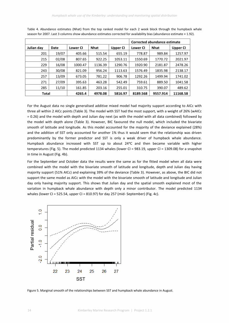
For the August data no single generalised additive mixed model had majority support according to AICc with

three all within 2 AICc points (Table 3). The model with SST had the most support, with a weight of 26% (wAICc

= 0.26) and the model with depth and Julian day next (as with the model with all data combined) followed by

the model with depth alone (Table 3). However, BIC favoured the null model, which included the bivariate

smooth of latitude and longitude. As this model accounted for the majority of the deviance explained (28%)

and the addition of SST only accounted for another 1% thus it would seem that the relationship was driven

predominantly by the former predictor and SST is only a weak driver of humpback whale abundance.

Humpback abundance increased with SST up to about 24ᵒC and then became variable with higher

temperatures (Fig. 5). The model predicted 1134 whales (lower CI = 983.19, upper CI = 1309.08) for a snapshot

in time in August (Fig. 4b).

For the September and October data the results were the same as for the fitted model when all data were

combined with the model with the bivariate smooth of latitude and longitude, depth and Julian day having

majority support (51% AICc) and explaining 39% of the deviance (Table 3). However, as above, the BIC did not

support the same model as AICc with the model with the bivariate smooth of latitude and longitude and Julian

day only having majority support. This shows that Julian day and the spatial smooth explained most of the

variation in humpback whale abundance with depth only a minor contributor. The model predicted 1134

whales (lower CI = 525.54, upper CI = 810.97) for day 257 (mid- September) (Fig. 4c).

Figure 5. Marginal smooth of the relationships between SST and humpback whale abundance in August.

Pa

rtia

l re

sid

ua

l

SST



3.2 Species distribution model

Distance to Coast and Depth were still correlated at 0.7 but they were left in as they both had varying degrees

of contribution to the resulting Maxent models and provided meaningful response curves. When all months

were combined, the most influential environmental/biophysical predictor of habitat suitability for humpback

whales in the Kimberley was distance to coast both for all whales (Fig. 6a) and for females with calves (Fig. 6b).

The same predictor emerged for the analysis of the data split into months of sampling (Fig. 6). For pods

containing females and calves the percentage contribution of distance to coast was slightly lower in August,

with SST making up the difference (Fig. 6b). Probability of presence dropped rapidly as distance to coast

increased, with a more rapid decline for pods with females and calves (Fig. 7). During August, probability of

presence of all whales and females with calves declined sharply when SSTs were greater than approx. 26ᵒC (Fig.

8a&b). Spatial predictions are shown in Figures 9 and 10. For all whales and for groups containing females and

calves only we found a seasonal shift in habitat suitability, which was lower at Camden Sound in June and July

(Fig. 9 and 10b) and September and October (Fig. 9 and 10 d) than in other months (Fig. 9b and c). When data

sets from all months were pooled, there were three main areas where habitat suitability was highest – the

coast of the Dampier Peninsula, Tasmanian Shoals and Camden Sound (Fig. 9 and 10a). The Tasmanian Shoal

area was not as important for groups containing females and calves (Fig. 10a). This pattern was more obvious

when we converted continuous (0-1) SDM output (habitat suitability) to a binary scale (suitable and unsuitable)

using the application of the thresholding method. Although this process results in loss of spatial information

and is dependent on the threshold selected (Wilson 2011), it is useful in this context of assessing the difference

in habitat use between the two groups. Groups with females and calves preferred habitat closer to the coast at

Pender Bay and along the Dampier Peninsula between Pender Bay and Broome, whereas when data for all

groups were pooled, suitable habitat extended further from shore and included a much larger area in

Tasmanian Shoal and Camden Sound (Fig. 11). Model evaluation showed that the model performed relatively

well (Table 5). All models had high mean AUC scores with low AUC variance, high TSS scores indicating

predicted probabilities from tuned models fit well with testing datasets, denoting a reliable prediction based on

occurrence datasets.

Figure 6. Variable contribution scores from the MaxEnt model on all months combined and each of the three monthly

datasets for all whale groups combined (a) and groups with females and calves only (b).



Figure 7. Maxent model response curves for each of the top predictor (distance to coast) in the model for all whale groups

for all months combined (a) and for pods with females and calves only for all months combined (b). Response curves

represent the change in probability of presence in chosen predictor variable while all other variables are kept at median

values.

Figure 8. MaxEnt model response curves for SST in August for whale pods combined (a) and pods with females and calves

(b). Response curves represent the change in probability of presence in chosen predictor variable while all other variables

are kept at median values.



Figure 9. MaxEnt model output (clog-log representation) showing habitat suitability for all whale groups in all months

combined (a), June and July (b), August (c) and September and October (d). Black lines show the State of Western

Australia’s Kimberley Marine Parks. See appendix 1 for the names of each of the parks.



Figure 10. MaxEnt model output (clog-log representations) showing habitat suitability for females and calves in all months

combined (a), June and July (b), August (c) and September and October (d). See caption for Fig. 9 for further details



Figure 11. Model estimated suitable and unsuitable habitat mapped for all observations (a), groups containing females and

calves (b) and the overlap between these two (c). Thresholding of models were conducted using maximum kappa threshold

for all models. See caption for Fig. 9 for further details

Table 5. Model evaluation results. AUC = area under the curve.

AUCmean ± AUCvar Kappa True Skill Statistic

All groups

All months 0.89 ± 0.01 0.53 0.61

June and July 0.92 ± 2x10-2 0.49 0.70

August 0.88 ± 0.01 0.46 0.59

Sept and Oct 0.89 ± 0.01 0.46 0.63

Cow-calf groups

All months 0.88 ± 0.01 0.35 0.59

June and July 0.90 ± 0.04 0.47 0.70

August 0.87 ± 0.02 0.46 0.57

Sept and Oct 0.89 ± 4x10-2 0.37 0.61



3.3 Humpback whale movement behaviour

The results from the state-space switching model applied to the satellite tracking data for individual whales

showed that while in the Kimberley region, humpback whales were almost always in resident mode, i.e. not

migrating. Even though some short, transitory movements appeared to be visible in the tracks (e.g. from

Camden Sound to Tasmanian Shoal and Pender Bay), the model did not identify a switch in behaviour, which

matches with expectations, given that the animals use the area for breeding. However, most of the tracks were

very short (median = 13 d, table 2), so that a switch in behaviours between resident and transient modes may

have been harder to detect. Only two whales showed a switch to transient mode (96382 and 96389 from

2009), with each of these having deployment durations of 60 and 33 days respectively. This switch occurred

around Exmouth and at the end of Eighty Mile Beach respectively. A total of 15 of the individual tracks were

too short and some had gaps in the data, resulting in failures of the state-space model. For this reason, we used

the raw location data in the analysis of time spent per grid cell (Fig. 12). Northbound whales used areas further

from shore (69 ± 71 km) (Fig. 12a) than southbound whales (36 ± 31 km) (Fig. 12 b). When examining the

histogram of distances to shore (Fig. A2), northbound whales had a much larger range, and appeared to have

two modes; the main one around 30 km and a second smaller one around 225 km (Fig. A2). The most heavily-

used areas in the Kimberley region on the northward migration were James Price Point, offshore of the

southern part of the Dampier Peninsula and Tasmanian Shoal (Fig. 12a) and Pender Bay and the norther part of

the Dampier Peninsula on the southward migration (Fig. 12b). For both migrations Eighty Mile Beach also had

some residency (Fig. 12).



Figure 12. Number of days spent by northbound (a) and southbound (b) humpback whales per 10 km × 10 km grid cell,

calculated from raw Argos location data from tagged humpback whales from 2008, 2009 and 2011. Grey lines show the 25

m, 50 m, 100 m, 500 m and 1000 m depth contours. Note that only the Kimberley region is shown, even though time spent

was calculated across the whole spatial extent.



4 Discussion

Our analysis of all available survey data for humpback whales across the nearshore waters of the Kimberley

region quantified seasonal shifts in abundance and habitat suitability and revealed the importance of inshore

areas for females and calves. Importantly, the spatio-temporal distribution maps produced by the analysis will

be useful for evaluation of the potential effects of current and proposed human activities on humpback whales

in the Kimberley.

Three of the aerial survey datasets were collected with estimation of long-term (multi-year) density

distributions as an objective and had the inputs needed for density surface modelling. These data are now

almost ten years old and, given a population increase estimated to be in the order of 11% per year (Salgado-

Kent et al. 2012), it is likely that current abundance would be higher than the abundance estimates calculated

here. However, relative patterns in density among areas will still be useful. The top predictors of abundance

were depth and day of year, with the model predicting numbers to increase up to mid-August and to peak in

waters around 35 m depth and decline in waters shallower than 25 m. Similarly, humpback whales on the Great

Barrier Reef also had a preference for waters between 30-58 m deep (Smith et al. 2012). The decline in

abundance in the Kimberley after mid-August concurs with whaling data, which suggests that at this time most

animals are migrating out of the breeding grounds (Chittleborough 1965). The model also predicted an

increasing trend in abundance with survey year, although spatial and temporal survey effort increased with

year so this almost certainly affected this result, as predicted abundances were much greater (up to 40%) than

previously reported (11% per annum). The trend is however still consistent with that reported for this

increasing population of humpback whales (Salgado-Kent et al. 2012). Our total abundance estimate for the

season (~10,000) was much less than the ~30,000 for the total WA population. While there is evidence to

suggest that whales calve in other areas along the coastline and do not all travel to the Kimberley (Irvine et al.

2017), it is important to note that our abundance estimates were only for the surveyed region which did not

include the entire area used by humpbacks in the Kimberley. The satellite tracking data (and the surveys to

Scott Reef) show that the whales occupy a much larger area of the Kimberley than was surveyed by plane and

used in the density surface models and given that the season might start in mid-June (Blake et al. 2011) and

extend to mid-November but might differ in timing among years by three weeks (Jenner et al. 2001) our

estimates (calculated from mid-July to mid-October) are most certainly an underestimate. In addition, our

season abundance estimate was based on the assumption that the average length of stay in the Kimberley is

two weeks (calculated from mark-recapture from photo ID of 35 whales in the Kimberley). However as there is

likely to be variation in the length of stay among sexes and classes of whales (Jenner & Jenner 2007b), our

whole of season estimate will further be under-estimated if whales stay less than two weeks.

The abundance model using all data combined identified Pender Bay as a principal core area of habitat for

humpback whales, although other areas such as Camden Sound, the Buccaneer Archipelago/Tasmanian Shoals

region and Gourdon Bay were also important. When the data for August and for September/October were

analysed separately it was possible to detect a seasonal shift in abundance with Camden Sound, Gourdon Bay

and the Tasmanian Shoal areas more important in August than in September and October. Interestingly,

Gourdon Bay is at the southern end of the survey region so it might be expected that it would be more

important later in the season than August, however this was also reported by Jenner and Jenner (2009). Pender

Bay became the principal core area in the latter months of September and October. Although these areas have

all been previously identified as important (Jenner et al. 2001), our models have quantified their relative

importance. This seasonal shift matches the previously reported migration pattern (Chittleborough 1965,

Dawbin 1997) whereby mothers and calves are reported to be at the rear of the migration and by the time

calves appear in August, much of the non-calving population have already started heading south. As Camden

Sound is at the northern extent of the migration for this humpback population (Jenner et al. 2001) it starts to

‘empty out’ before the more southern locations.

Distance to coast was the most important predictor of habitat suitability for humpback whales, with the

majority of individuals sighted within 20-40 km of the coast. This behaviour may offer both respite from the



strong tidal currents of the Kimberley and assistance with swimming, and might be especially important for an

animal living on a fixed energy budget (humpbacks do not feed during the migration). Distance to coast was

also important for abundance patterns of humpback whales on the Great Barrier Reef (Smith et al. 2012),

although depth and SST were more important as determinants of distribution on the east coast than the west.

Off the Kimberley, SST was only important in August, with whales displaying a preference for temperatures

around 24.5 and 26.5ᵒC, within the range of temperatures (21 - 28ᵒC) reported for the species worldwide

(Rasmussen et al. 2007). This coincides with the peak of parturition (early August) for this population

(Chittleborough 1958) and both models (abundance and presence/absence models) showed Camden Sound, an

area considered a major calving ground (Jenner et al. 2001), as important during this month. Perhaps the

combination of slower tidal currents as evidenced by generally lower turbidity (Fig. A3) mentioned above and

the consequent higher water temperatures make Camden Sound an ideal calving ground. Camden Sound is also

an important area for all groups in August, not just groups with caves. Mature males also likely to concentrate

here since there is an aggregation of successful breeding females in August, particularly since some of these

female whales may come into post-partum oestrus.

Sea surface temperature did not emerge as an important predictor of abundance of humpback whales (density

surface models) when all data were combined, however when Julian day was not included as a predictor in the

models, SST did emerge in the top model. Given that the addition of Julian day forced SST to be dropped from

the top model, it suggests that the animals are not basing their movements on SST but instead on some other

covariate for which time is a better proxy. It is also possible that they do move explicitly according to time, for

example for position of the sun or day length perhaps. Additionally, at local scales, less than optimal water

temperature might be selected if those areas offer suitable, shallow protected conditions (Rasmussen et al.

2007), especially for females and calves trying to avoid the attention of males. This might explain why SST was

only a weak predictor in the models for August and that requirements might change as the season progresses.

For example the relationship between mother-calf pairs and water depth and sea bed terrain changed with calf

age (Pack et al. 2017).

The species distribution models predicted similar core areas to the density surface model, however Camden

Sound, the Tasmanian Shoal area and the entire coast of the Dampier Archipelago were all equally important

across the season. Analysis of each of the three time periods showed that Camden Sound was only important in

August, a result consistent with abundance models. Importantly, the models predict habitat suitability of

groups with females and calves in June and July south of the Lacepede Islands, and in August, habitat suitability

includes the coast of the Dampier Peninsula, not just Camden Sound. This suggests that the calving grounds

extend beyond the Camden Sound area. New evidence suggests that calving areas for humpbacks extends

along a substantial part of the migratory corridor along Western Australia, rather than being confined to

discrete, localised areas (Irvine et al. 2017). As recorded by earlier studies (Craig & Herman 2000, Irvine et al.

2017), habitat preference differed between breeding (those without calves) and calving/nursing groups (those

with calves present) with calving areas closer to shore and less extensive than breeding areas. As mentioned

above, females and calves may prefer shallower, protected habitat which might also be warmer. In addition,

highly competitive groups of males often chase cow-calf groups through and around Camden Sound, such that

females with calves may be forced closer to shore or may stay as close to the coast as possible to avoid

detection.

Evaluation showed that the species distribution model performed relatively well and that its predictions were

reliable. In addition, the areas of importance to humpbacks identified by the model were consistent with

satellite tracking data, which showed a similar area of importance across the Kimberley although not extending

as far as Broome and with only moderate use of Camden Sound. This latter issue might be more to do with

biases in the tracking data than actual patterns of use, since many of the transmitters on northbound whales

tracked from NW Cape in 2011 had ceased reporting positional data before tagged individuals arrived in the

Kimberley (only 8 of 23 tags were still transmitting on arrival in the Kimberley) and that the southbound whales

were mostly tagged south of Camden Sound. However, of the eight whales that arrived in Kimberley in 2011,



only four went to Camden Sound and in 2006 when six northbound whales were tagged at James Price Point,

only two went to Camden Sound. As suggested previously (Jenner 2001), northbound whales migrated further

offshore than southbound whales and the raw Scott Reef survey data that we were unable to model shows that

humpback whales use areas beyond what was modelled here. Although the majority of the area used by the

majority of the population using the Kimberley has been modelled.

Pender Bay was identified by both modeling approaches to be an important core area for humpback whales in

the Kimberley. It is important to note that this may be partly related to Pender Bay being a physical gateway

into, and out of, the Kimberley calving area. Humpback whales are not thought to migrate continuously in this

region and as Pender Bay is also a shallow area out of the tidal current, whales may rest here before advancing

both inbound to and outbound from the Kimberley and Camden Sound. This two-way traffic could create a

pattern of higher abundances of whales in Pender Bay across the season. This contrasts with Camden Sound

and the neighbouring Buccaneer Archipelago at the northern extent of the breeding grounds, where it is

thought that cow-calf groups do not linger for more than 1-2 weeks (Jenner et al. 2001). Tasmanian Shoals also

has “two-way traffic”, but to a lesser extent since whales disperse once they are north of Pender Bay and some

move slightly south into the islands of the Buccaneer Archipelago. The importance of Pender Bay as a resting

area (Jenner et al. 2001) and the very high abundances of humpbacks that occur here over the entire breeding

season suggest that it should be given consideration for additional protection measures.

Importantly, there have not been any systematic surveys of the Kimberley region, including Camden Sound

since an aerial survey by CWR in 2007. While it is widely recognised that the population has been increasing

each year as it recovers from the decimation of whaling, there is no current estimate of the absolute

population size nor of how population growth may have affected spatial use in the important breeding grounds

of the Kimberley. It is now crucial that a monitoring program be implemented to ensure this population is

managed effectively into the future, given the growing pressures of climate change and other anthropogenic

pressures in the marine environment. Differences in the spatial and temporal coverage of the datasets

compiled and analysed here, prevented valid/robust analysis and detection of trends among years and

highlights the importance of having, long-term, repeatable systematic survey data to effectively monitor

trends.



5 References

Bailey H, Mate BR, Palacios DM, Irvine L, Bograd SJ, Costa DP (2009) Behavioural estimation of blue whale movements in the Northeast Pacific from state-space model analysis of satellite tracks. Endangered Species Research 10:93-106

Bailey H, Shillinger G, Palacios D, Bograd S, Spotila J, Paladino F, Block B (2008) Identifying and comparing phases of movement by leatherback turtles using state-space models. Journal of Experimental Marine Biology and Ecology 356:128-135

Barlow J, Oliver CW, Jasckson TD, Taylor BL (1988) Harbor porpoise, Phocoena phocoena, abundance estimation for California, Oregon, and Washington: II. Aerial surveys. Fisheries Bulletin 86:433-444

Blake S, Dapson I, Auge O, Bowles A, Marohn E, Malatzky L, Saulnier S (2011) Monitoring of Humpback Whales in the Pender Bay, Kimberley Region, Western Australia, Vol 94

Buckland ST, Anderson DR, Burnham KP, Laake JL, Borchers DL, Thomas L (2011) Introduction to distance sampling: estimating abundance of biological populations, Vol. Oxford University Press Inc., New York, United States

Burnham KP, Anderson DR (2002) Model selection and multimodel Inference: a practical information-theoretic approach, Vol. Springer-Verlag, New York

Cartwright R, Sullivan M (2009) Behavioral ontogeny in humpback whale (Megaptera novaeangliae) calves during their residence in Hawaiian waters. Marine Mammal Science 25:659-680

Chittleborough R (1965) Dynamics of two populations of the humpback whale, Megaptera novaeangliae (Borowski). Marine and Freshwater Research 16:33-128

Chittleborough RG (1953) Aerial Observations on the Humpback Whale, Megaptera nodosa (Bonnaterre), with Notes on Other Species. Marine and Freshwater Research 4:219-226

Chittleborough RG (1958) The breeding cycle of the female humpback whale, Megaptera nodosa (Bonnaterre). Marine and Freshwater Research 9:1-18

Costa DP, Breed GA, Robinson PW (2012) New insights into pelagic migrations: implications for ecology and conservation. Annual Review of Ecology and Systematics 43:73-96

Costa DP, Robinson PW, Arnould JPY, Harrison A-L, Simmons SE, Hassrick JL, Hoskins AJ, Kirkman SP, Oosthuizen H, Villegas-Amtmann S, Crocker DE (2010) Accuracy of ARGOS locations of pinnipeds at-sea estimated using fastloc GPS. PLoS ONE 5(1): e8677

Craig AS, Herman LM (2000) Habitat preferences of female humpback whales Megaptera novaeangliae

in the Hawaiian Islands are associated with reproductive status. Marine Ecology Progress Series 193:209-216

Dawbin WH (1997) Temporal segregation of humpback whales during migration in southern hemisphere waters. Memoirs of the Queensland Museum 42:105-138

Double MC, Gales N, Jenner KCS, Jenner M-N (2010) Satellite tracking of south-bound female humpback whales in the Kimberley region of Western Australia. Final Report

Double MC, Jenner KCS, Jenner M-N, Ball I, Childerhouse S, Laverick S (2011) Satellite tracking of northbound humpback whales (Megaptera novaeangliae) off Western Australia. Draft Final Report - December 2011

Fabricius K, De'ath G (2000) Biodiversity on the Great Barrier Reef. In: Wolanski E (ed) Oceanographic Processes of Coral Reefs. CRC Press

Irvine LG, Thums M, Hanson CE, McMahon CR, Hindell MA (2017) Evidence for a widely expanded humpback whale calving range along the Western Australian coast. Marine Mammal Science 10.1111/mms.12456

Jenner KCS, Jenner M-N (2007a) Browse Basin Cetacean Monitoring Programme 2006 Season Report. Unpublished report to Inpex Browse Pty Ltd

Jenner KCS, Jenner M-N (2007b) Browse Basin Cetacean Monitoring Programme 2007 Season Report. Unpublished report to Inpex Browse Pty Ltd and the Department of Environment Water Heritage and the Arts

Jenner KCS, Jenner M-N (2009) Humpback Whale Distribution and Abundance in the Near Shore SW Kimberley During Winter 2008 Using Aerial Surveys. Unpublished report to Woodside Energy and the Northern Development Taskforce

Jenner KCS, Jenner M-N, McCabe KA (2001) Geographical and temporal movements of humpback whales in Western Australian waters. APPEA Journal 38:692-707

Jonsen ID, Basson M, Bestley S, Bravington MV, Patterson TA, Pedersen MW, Thomson R, Thygesen UH, Wotherspoon SJ (2013) State-space models for bio-loggers: a methodological road map. Deep Sea Research II 88-89:34-46

Jonsen ID, Flenming JM, Myers RA (2005) Robust state-space modeling of animal movement data. Ecology 86:2874-2880

Jonsen ID, Myers RA, Flemming JM (2003) Meta-analysis of animal movement using state-space models. Ecology 84:3055-3063

Kareiva P, Odell G (1987) Swarms of predators exhibit prey taxis if individual predators use area-restricted search



American Naturalist 130:233-270

Kaufman GD, Forestell PH (2006) Hawaii's Humpback Whales. Island Heritage Publishing, Hawaii:25

Lerczac JA, Hobbs R (2006) Calculating sighting distances from angular readings during shipboard, aerial, and shore-based marine mammal surveys. Marine Mammal Science 14:590-598

Miller DL (2017a) Density surface modelling of distance sampling data 2.2.15. http://githubcom/DistanceDevelopment/dsm

Miller DL (2017b) Distance sampling detection function and abundance estimation 0.9.7. http://githubcom/DistanceDevelopment/Distance/

Miller DL, Burt ML, Rexstad EA, Thomas L (2013) Spatial models for distance sampling data: recent developments and future directions. Methods in Ecology and Evolution 4:1001-1010

Muscarella R, Galante PJ, Soley-Guardia M, Boria RA, Kass JM, Uriarte M, Anderson RP (2017) Automated runs and evaluations of ecological niche models 0.2.2. CRAN

Pack AA, Herman LM, Craig AS, Spitz SS, Waterman JO, Herman EYK, Deakos MH, Hakala S, Lowe C (2017) Habitat preferences by individual humpback whale mothers in the Hawaiian breeding grounds vary with the age and size of their calves. Animal Behaviour 133:131-144

Phillips SJ, Anderson RP, Schapire RE (2006) Maximum entropy modeling of species geographic distributions. Ecological Modelling 190:231-259

Plummer M JAGS: A Program for Analysis of Bayesian Graphical Models Using Gibbs Sampling. In. Proc Proceedings of the 3rd International Workshop on Distributed Statistical Computing (DSC 2003)

R Core Team (2017) R: A language and environment for statistical computing. In. R Foundation for Statistical Computing Vienna, Austria

Rasmussen K, Palacios DM, Calambokidis J, Saborío MT, Dalla Rosa L, Secchi ER, Steiger GH, Allen JM, Stone GS (2007) Southern Hemisphere humpback whales wintering off Central America: insights from water temperature into the longest mammalian migration. Biology Letters 3:302-305

RPS Environment and Planning Pty Ltd (2010) Humpback whale survey report. Browse MMFS 2009

Salgado-Kent CP, Jenner KCS, Jenner M, Rexstad EA (2012) Southern Hemisphere breeding stock ‘D’ humpback whale population estimates from North West Cape, Western Australia. Journal of Cetacean Research and Management 12:29-38

Smith JN, Grantham HS, Gales N, Double MC, Noad MJ, Paton D (2012) Identification of humpback whale breeding and calving habitat in the Great Barrier Reef. Marine Ecology Progress Series 447:259-272

Wilson PD (2011) Distance-based methods for the analysis of maps produced by species distribution models. Methods in Ecology and Evolution 2:623-633

http://githubcom/DistanceDevelopment/dsm

http://githubcom/DistanceDevelopment/Distance/


Michele Thums1,5, Curt Jenner2,5, Kelly Waples3,5, Chandra Salgado-Kent4,5, Mark

Meekan1,5

1Australian Institute of Marine Science, Perth, Western Australia, Australia

2Centre for Whale Research, Perth, Western Australia, Australian Institute of Marine Science

3Western Australia Department of Biodiversity, Conservation and Attractions, Perth, Western Australia, Australia

4Curtin University, Centre for Marine Science and Technology, Perth, Western Australia 5Western Australian Marine Science Institution (WAMSI), Perth, Western Australia, Australia

WAMSI Kimberley Marine Research Program

KMRP Report

Project 1.2.1

July 2018

Documents

Chapter 1: Modelling the movement and spatial distribution