Embed Size (px)
Citation preview

17/4/13
Challenge the future Delft University of Technology
CIE4801 Transportation and spatial modelling
Rob van Nes, Transport & Planning
Spatial modelling: concept and descriptive models

2 CIE4801: Spatial modelling 1
• Two topics in balance? • Transportation modelling 14 lectures • Spatial modelling 2.5 lectures
• Three reasons • Main expertise T&P • Similar modelling aproaches • Interaction within transport system is
dominant
• Expertise within T&P • 3 PhD-studies • Dr.ir. R. Verhaeghe
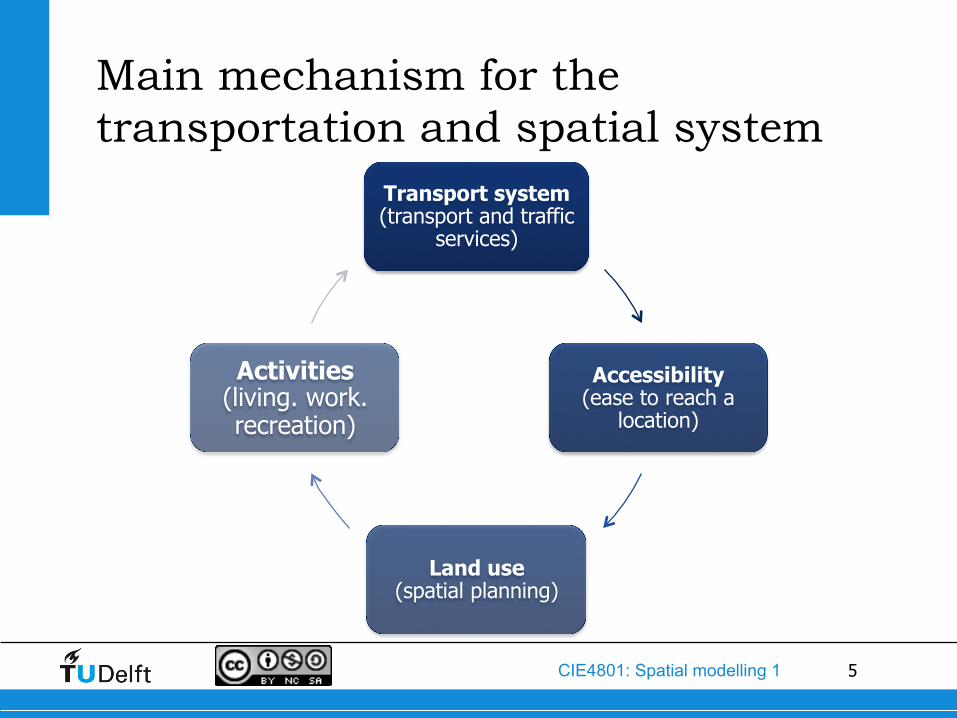
Transportation & spatial modelling
Transport system
(transport and traffic services)
Accessibility (ease to reach a
location)
Land use (spatial planning)
Activities (living. work. recreation)

3 CIE4801: Spatial modelling 1
Content
• Background • Early (economic) models • Some empirical findings
• Descriptive models • Accessibility • Hansen • Lowry • Immers & Hamerslag
• Land use and transportation models (Tuesday) • TIGRIS XL • Choice modelling for household and firm allocation

4 CIE4801: Spatial modelling 1
2.
Background: classical models
5 CIE4801: Spatial modelling 1
Main mechanism for the transportation and spatial system
Transport system (transport and traffic
services)
Accessibility (ease to reach a
location)
Land use (spatial planning)
Activities (living. work. recreation)

6 CIE4801: Spatial modelling 1
Single commodity model • (large number of) producers want to sell a certain agricultural
commodity a central market place • (large number of) owners rent land to the producers • land owners let the producers bid on the land space • producers will bid a rent with which they still can make profits Question: What rents will the producers pay for the land, and how much land will be used?
land used by producer
central market
?
Classical models: Von Thunen (1826)
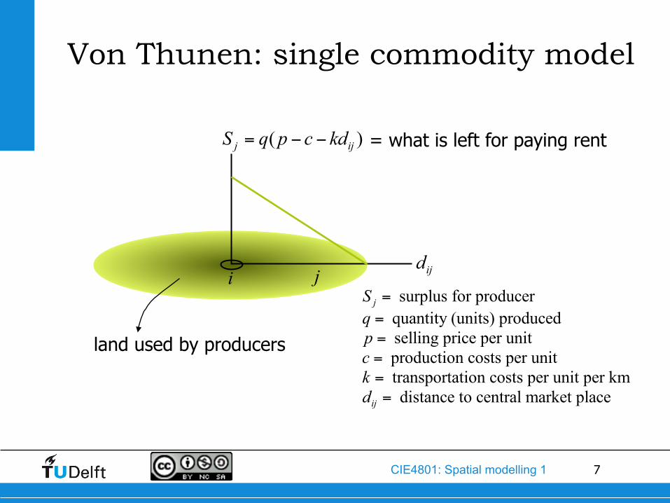
7 CIE4801: Spatial modelling 1
i j surplus for producer
quantity (units) produced selling price per unit production costs per unit transportation costs per unit per km distance to central market place
======
j
ij
Sqpckd
( )= − −j ijS q p c kd
ijd
= what is left for paying rent
land used by producers
Von Thunen: single commodity model
8 CIE4801: Spatial modelling 1
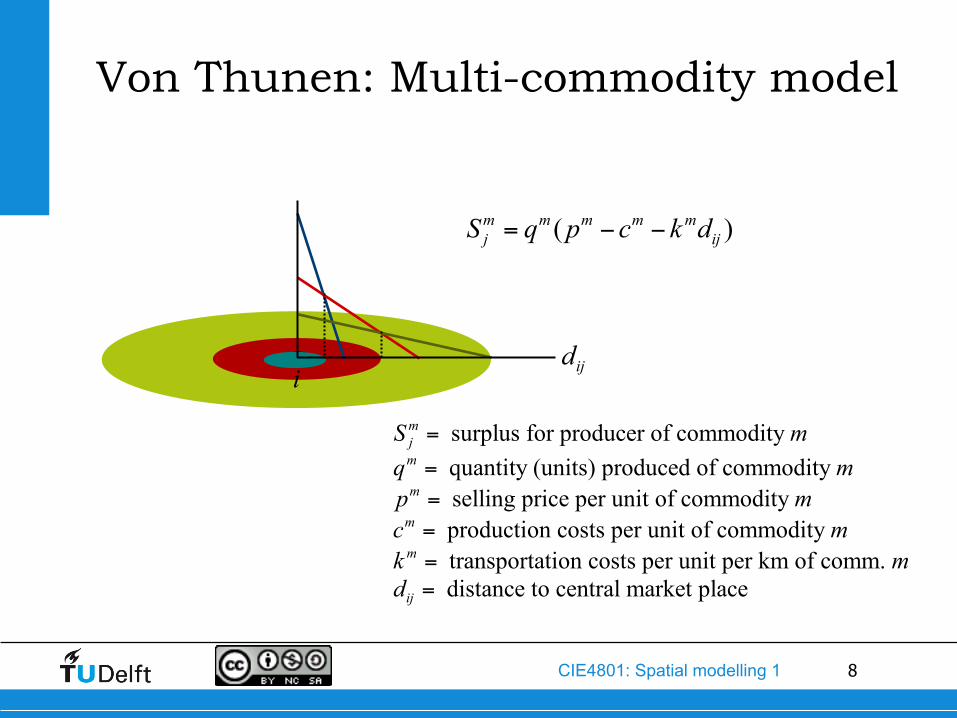
surplus for producer of commodity quantity (units) produced of commodity selling price per unit of commodity production costs per unit of commodity transportation costs per un
=
====
mjm
m
m
m
S mq mp mc mk it per km of comm.
distance to central market place=ij
md
( )= − −m m m m mj ijS q p c k d
ijdi
Von Thunen: Multi-commodity model

9 CIE4801: Spatial modelling 1
Classical models: Christaller (1932)

10 CIE4801: Spatial modelling 1
• evenly distributed population of self-sufficient farmers • farmers can produce beer for a certain area
producing for a larger area: - cheaper production process - more expensive distribution
Classical models: Christaller (1932)
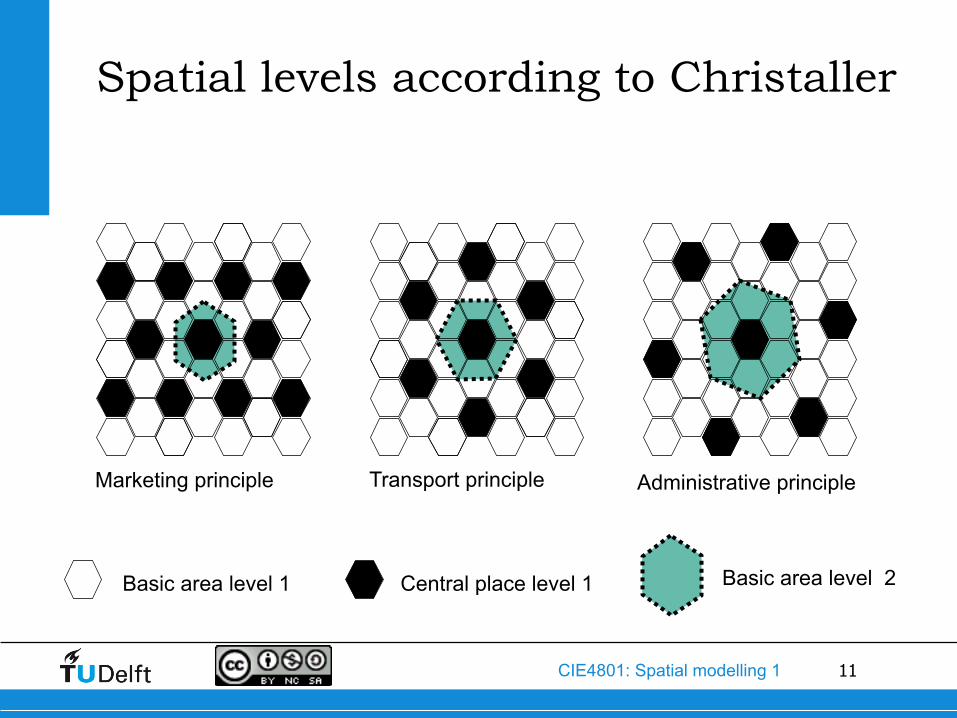
11 CIE4801: Spatial modelling 1
Spatial levels according to Christaller
Administrative principle Transport principle Marketing principle
Basic area level 1 Central place level 1 Basic area level 2

12 CIE4801: Spatial modelling 1
Morphological perspective
• Every level shows new details
Dispersion or maximal homogeniety
Concentration or minimal homogeniety

13 CIE4801: Spatial modelling 1
One of many possible classifications
Name Radius [km]
Surface [km2]
Inhabitants
Village 0,3 0,3 1.000
Town 1 3 10.000
City 3 30 100.000
Agglomeration 10 300 1.000.000
Metropolis 30 3.000 10.000.000

14 CIE4801: Spatial modelling 1
Classical models: Hotelling
15 CIE4801: Spatial modelling 1
Agglomeration factors
• Advantages of agglomerations
• Positive externalities
• Associated development
• Education, health care, financial services
• Transport is essential
• Congestion limits growth of agglomerations

16 CIE4801: Spatial modelling 1
3.
Some empirical findings
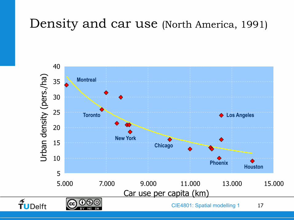
17 CIE4801: Spatial modelling 1
5
10
15
20
25
30
35
40
5.000 7.000 9.000 11.000 13.000 15.000 Car use per capita (km)
Urb
an d
ensi
ty (
pers
./ha
)
Houston
Montreal
Toronto
Chicago New York
Los Angeles
Phoenix
Density and car use (North America, 1991)
18 CIE4801: Spatial modelling 1
19 CIE4801: Spatial modelling 1

20 CIE4801: Spatial modelling 1

21 CIE4801: Spatial modelling 1

22 CIE4801: Spatial modelling 1
23 CIE4801: Spatial modelling 1
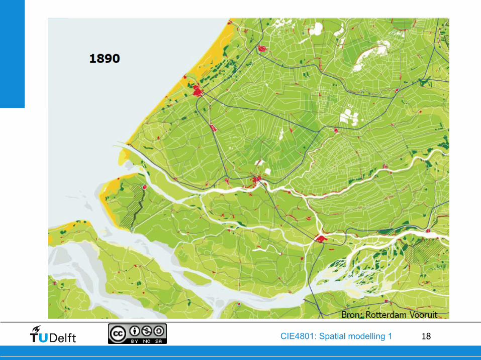
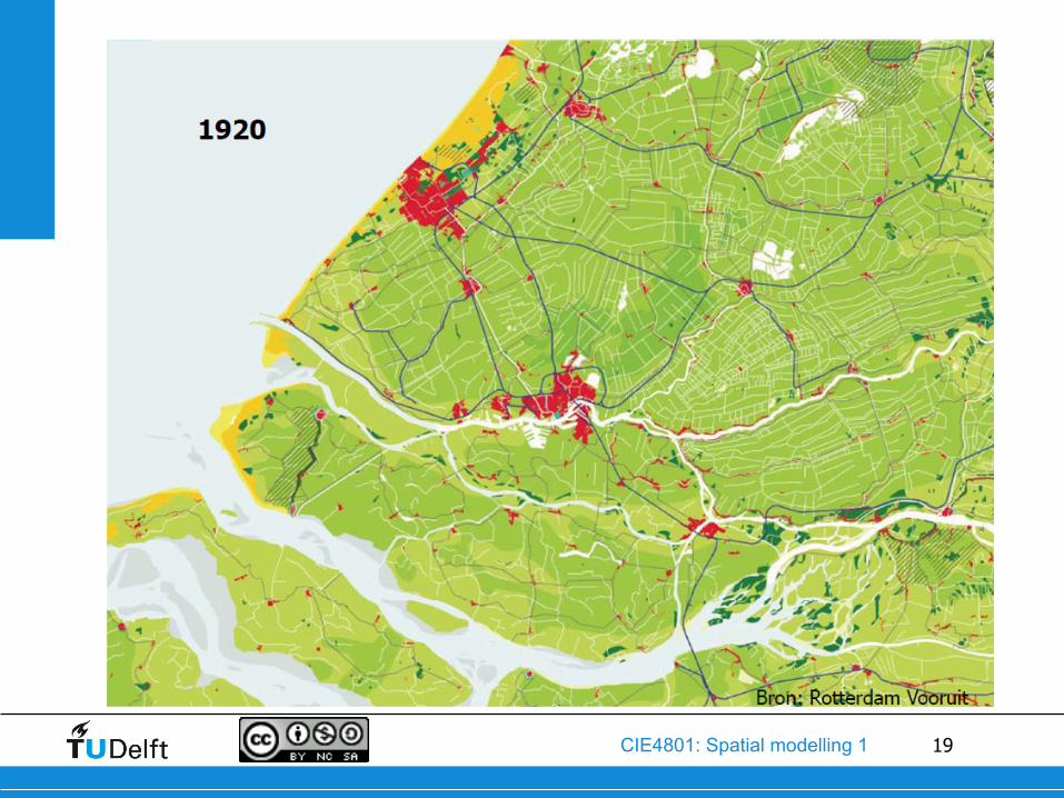
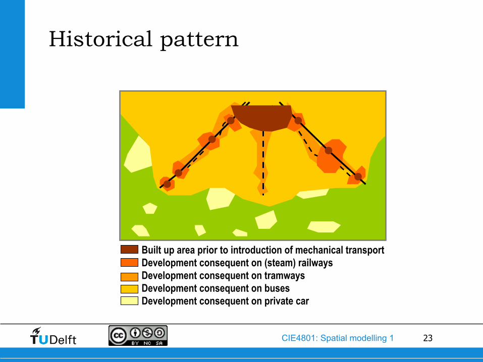
Built up area prior to introduction of mechanical transport Development consequent on (steam) railways Development consequent on tramways Development consequent on buses Development consequent on private car
Historical pattern
24 CIE4801: Spatial modelling 1
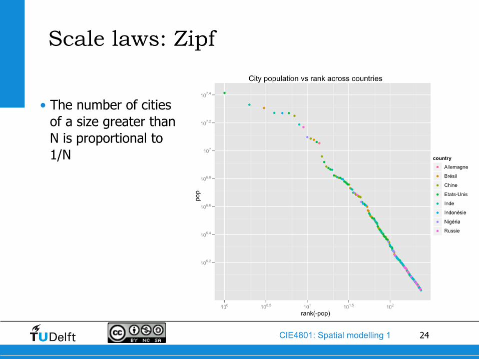
• The number of cities of a size greater than N is proportional to 1/N
Scale laws: Zipf

25 CIE4801: Spatial modelling 1
• Local conditions play a major role for the location of settlements • Safety • Water and food • Natural resources • Accessibility
• Mechanisms/drivers change over time • Other drivers might take over
• Law of increasing returns • Drivers may loose importance
• Stand-still or decline • Permanent or temporary
Settlement patterns are also determined by chance

26 CIE4801: Spatial modelling 1
2.
Accessibility
27 CIE4801: Spatial modelling 1
Choice destina-
tion
Choice mode
Choice route/time
Travel time & costs
Accessibility
Attractiveness
Choice location
investors
Build
Choice location
users
Move
Activities
Ability to travel
Choice trip
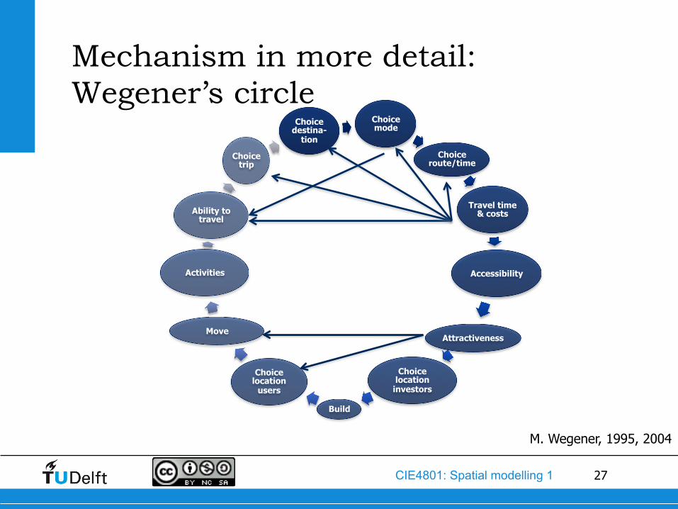
Mechanism in more detail: Wegener’s circle
M. Wegener, 1995, 2004

28 CIE4801: Spatial modelling 1
Definitions of accessibility?
• Ease to reach a location……..
• From where • Specific location? • From all locations? • From all locations within a certain distance/travel time? • ……
• By whom? • Individuals/households/companies at that location? • Possible clients/workforce? • ……….

29 CIE4801: Spatial modelling 1
Generic indicator: Potential value
• Sum of all clients/jobs/etc. that can be reached within a certain distance/time:
• Different options for f(cij):
( )( ) max, :i j ij ijj
PV g M f c j c c= ⋅ ⋅ ∀ ≤∑
( )
( ) ij ij
ij ij i j ijj
c cij i j
j
f c c PV g M c
f c e PV g M eβ β− −
= ⇒ = ⋅ ⋅
= ⇒ = ⋅ ⋅
∑
∑ Maximum is best?
Minimum is best?

30 CIE4801: Spatial modelling 1
• Choice for M depends on perspective • Active accessibility: where you can go to
e.g. the number of jobs you can reach from your home • Passive accessibility: who can reach you
e.g. number of clients that can reach you
• Choice for cij: • Time, distance, generalised costs, logsum over modes….
• Notice the similarity with trip distribution topics
So what to use for the atributes?

31 CIE4801: Spatial modelling 1
4.1
Descriptive models: Hansen-model

32 CIE4801: Spatial modelling 1
• Given the network and the location of the jobs
• What is the location of the inhabitants?
• Main assumption: people prefer a location having the highest accessibility
• However, there’s not always enough space available
What is it for?
33 CIE4801: Spatial modelling 1
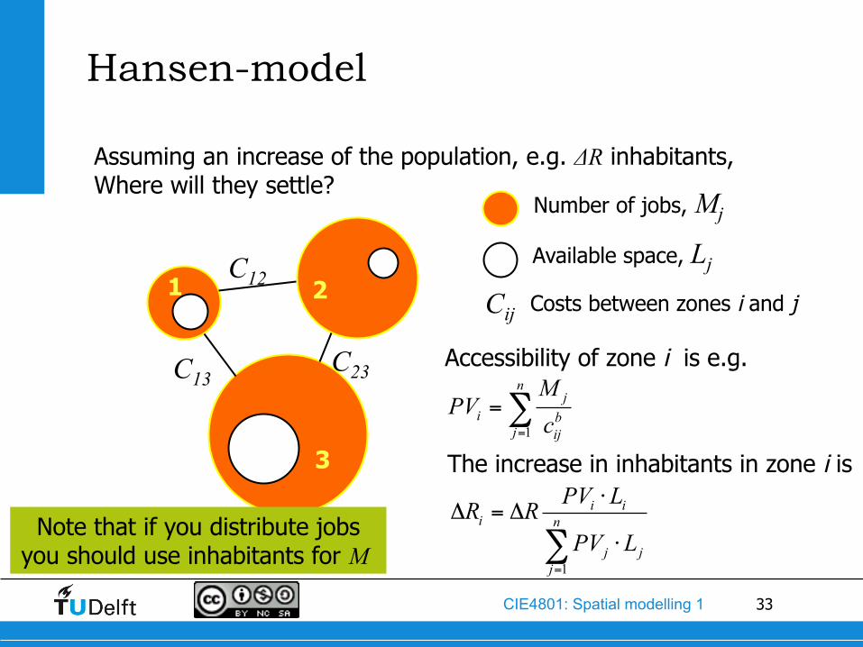
Hansen-model
Assuming an increase of the population, e.g. ΔR inhabitants, Where will they settle?
Number of jobs, Mj
Available space, Lj
Costs between zones i and j Cij 1 2
3
C12
C23 C13 Accessibility of zone i is e.g.
1
nj
i bj ij
MPV
c=
=∑
The increase in inhabitants in zone i is
1
i ii n
j jj
PV LR RPV L
=
⋅Δ = Δ
⋅∑Note that if you distribute jobs
you should use inhabitants for M

34 CIE4801: Spatial modelling 1
4.2
Descriptive models: Lowry-model

35 CIE4801: Spatial modelling 1
Lowry model: different type of jobs
• Distinction between basic jobs and service jobs • Basic jobs: location bound e.g. industry, government, • Service jobs: dependent on population e.g. education, health
care, retail
• Two main assumptions • Fixed ratio between population and jobs: u • Fixed ratio between service jobs and population: v
36 CIE4801: Spatial modelling 1
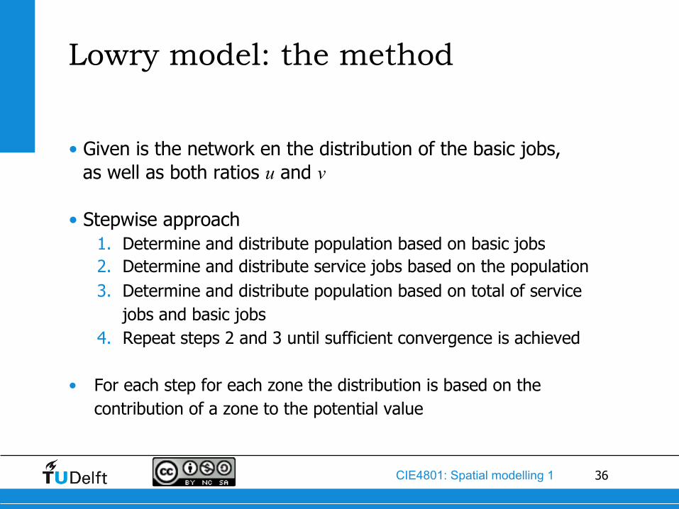
• Given is the network en the distribution of the basic jobs, as well as both ratios u and v
• Stepwise approach 1. Determine and distribute population based on basic jobs 2. Determine and distribute service jobs based on the population 3. Determine and distribute population based on total of service
jobs and basic jobs 4. Repeat steps 2 and 3 until sufficient convergence is achieved
• For each step for each zone the distribution is based on the contribution of a zone to the potential value
Lowry model: the method

37 CIE4801: Spatial modelling 1
Lowry-model: flow chart
Basic employment per zone
Service employment per zone
Total employment per zone
Number of inhabitants per zone
Inhabitant allocation
model
Service employment allocation
model
€
E jb s
jE
€
E j
€
Ri
Is equal to 0 for the first iteration

38 CIE4801: Spatial modelling 1
iR
jE
Lowry-model: Allocation inhabitants for workers in zone j
Cij
€
Li1
1
( )
( )
ii ij
ij j ni
k kjk
n
i ijj
L f cR u E
L f c
R R
=
=
⋅= ⋅
⋅
=
∑
∑
u = ratio between population and jobs Ej = total employment in j Ri = inhabitants in i Li = attractiveness for inhabitants in zone i cij = transport costs between i and j
Potential value of zone j

39 CIE4801: Spatial modelling 1
Ri
E js
Lowry-model: Allocation service jobs for zone i
Cij
Wj
( )( )
1
1
sj ijs
ij i ns
k ikk
ns sj ij
i
W f cE v R
W f c
E E
=
=
⋅= ⋅
⋅
=
∑
∑
v = ratio service jobs and population Es
j = service employment in j Ri = inhabitants in i Wj = attractiveness of j for service jobs cij = transport costs between i en j
In order to account for agglomeration effects Wj equals Es
j of the previous iteration

40 CIE4801: Spatial modelling 1
Concluding comments Lowry-model
• In every iteration the number of service jobs and thus the population increases
• As the algoritm convergences, it leads to an equilibirum • Rij is in fact the OD-matrix for commuters (i.e. when
corrected for u)

41 CIE4801: Spatial modelling 1
4.3
Descriptive models: Immers & Hamerslag

42 CIE4801: Spatial modelling 1
ij i j ijT Q X Fρ=
ij jiT A=∑
( ) ( )ij i j ij j i ij ji i iT Q X F X Q F Aρ ρ= = =∑ ∑ ∑
ij ijT P=∑
( ) ( )ij i j ij i j ij ij j jT Q X F Q X F Pρ ρ= = =∑ ∑ ∑
( )j
ji ij
i
AX
Q Fρ=∑( )
ii
j ijj
PQX Fρ
⇒ =∑
and
Recall the doubly constrained model
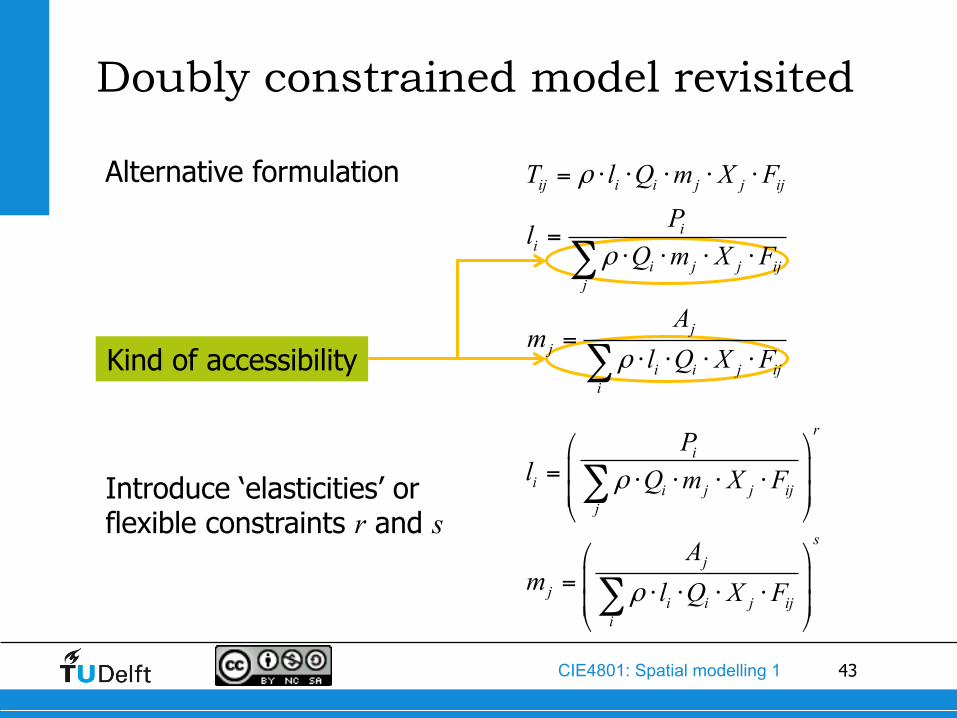
43 CIE4801: Spatial modelling 1
ri
i i j j ijj
sj
ji i j ij
i
Pl Q m X F
Am l Q X F
ρ
ρ
⎛ ⎞⎜ ⎟= ⋅ ⋅ ⋅ ⋅⎜ ⎟⎝ ⎠
⎛ ⎞⎜ ⎟= ⋅ ⋅ ⋅ ⋅⎜ ⎟⎝ ⎠
∑
∑
Doubly constrained model revisited
Alternative formulation
Kind of accessibility
Introduce ‘elasticities’ or flexible constraints r and s
ij i i j j ij
ii
i j j ijj
jj
i i j iji
T l Q m X FPl
Q m X F
Am
l Q X F
ρ
ρ
ρ
= ⋅ ⋅ ⋅ ⋅ ⋅
=⋅ ⋅ ⋅ ⋅
=⋅ ⋅ ⋅ ⋅
∑
∑

44 CIE4801: Spatial modelling 1
• In the standard model they make sure row totals equal the production and the column totals equal the attractions
• Their value is reversely related to the accessibility of the zone
• The production and attraction might not be considered as a hard constraint, e.g. because: • They’re an estimate • They might change due to the actual accessibility
• Note that if r and s equal 1, we have the doubly constrained model, and if one of them equals 0 we have the singly constrained model
Interpretation of balancing factors

45 CIE4801: Spatial modelling 1
• Model for the Randstad having zones of 150.000 inhabitants
• Reference case: everyone works in the zone they live
• Model with elastic constraints (r=-2, s=0.2) for evening peak (commuters only) • r=-2 suggests that highly accessible locations grow
(agglomeration effect) • s=0.2 suggests a limited effect of accessibility on residential
areas
• Model is implemented in an incremental procedure • Matrix update using elastic constraints (1 iteration) • Travel cost update
Example Immers & Hamerslag
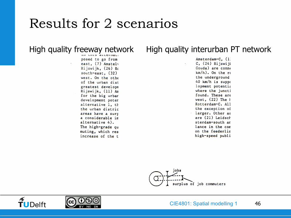
46 CIE4801: Spatial modelling 1
High quality interurban PT network
Results for 2 scenarios
High quality freeway network
47 CIE4801: Spatial modelling 1
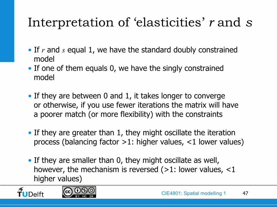
• If r and s equal 1, we have the standard doubly constrained model
• If one of them equals 0, we have the singly constrained model
• If they are between 0 and 1, it takes longer to converge or otherwise, if you use fewer iterations the matrix will have a poorer match (or more flexibility) with the constraints
• If they are greater than 1, they might oscillate the iteration process (balancing factor >1: higher values, <1 lower values)
• If they are smaller than 0, they might oscillate as well, however, the mechanism is reversed (>1: lower values, <1 higher values)
Interpretation of ‘elasticities’ r and s
48 CIE4801: Spatial modelling 1
• Values between 0 and 1 are justified • Unconstrained model • Singly constrained model • Models having flexible constraints
• Note that a limited number of iterations is required (e.g. the way it used in OD-estimation (see Lecture 9) where the
match with the a priori matrix is an important criterion) • Doubly constrained model
• Values smaller than 0 or greater than 1 are tricky • Effect depends on the ratio for li and mj
• Therefore: not recommended
Conclusion for ‘elasticities’