Embed Size (px)
Citation preview

Chapter 1
Affine algebraic geometry
We shall restrict our attention to affine algebraic geometry, meaning that thealgebraic varieties we consider are precisely the closed subvarieties of affine n-space defined in section one.
1.1 The Zariski topology on An
Affine n-space, denoted by An, is the vector space kn. We impose coordinatefunctions x1, . . . , xn on it and study An through the lens of the polynomial ringk[x1, . . . , xn] viewed as functions An → k.
First we impose topologies on An and k such that the polynomial functionsAn → k are continuous. We will require each point on k to be closed, andthis forces the fibers f−1(λ)An to be closed for each f ∈ k[x1, . . . , xn] and eachλ ∈ k. The set f−1(λ) = p | f(p) = λ is the zero locus of the polynomialf − λ; since every polynomial can be written in the form f − λ, the zero locusof every polynomial must be closed. Since a finite union of closed sets is closed,the common zero locus
p ∈ kn | f1(p) = · · · = fr(p) = 0
of every finite collection of polynomials f1, . . . , fr is closed. This is the definitionof the Zariski topology on An.
And the closed subsets of An are called affine algebraic varieties.A lot of important geometric objects are affine algebraic varieties. The conic
sections are the most ancient examples: the parabola is the zero locus of y−x2,the hyperbolas are the zero loci of equations like x2/a2−y2/b2−1, or more simplyxy − 1, the circles centered at the origin are the zero loci of the polynomialsx2+y2−r2, and so on. Higher-dimensional spheres and ellipsoids provide furtherexamples. Another example is the union in R4 of the xy-plane and wz-plane:it is the simultaneous zero locus of xw, xz, yw, and yz (or, more cleverly, ofxw, yz, and xz+yw). Fermat’s last theorem can be restated as asking whether,when n ≥ 3, the zero locus of the equation xn + yn − zn has any points withrational coordinates other than those in which one of the coordinates is zero.Another family of examples is provided by the n×n matrices over R having rank
1

2 CHAPTER 1. AFFINE ALGEBRAIC GEOMETRY
at most some fixed number d; these matrices can be thought of as the pointsin the n2-dimensional vector space Mn(R) where all (d + 1) × (d + 1) minorsvanish, these minors being given by (homogeneous degree d+1) polynomials inthe variables xij , where xij simply takes the ij-entry of the matrix.
We will write Ank for kn and call it affine n-space over k. For example, A1
is called the affine line and A2 is called the affine plane. We will only discussaffine algebraic geometry in this course. Projective algebraic geometry is a muchprettier subject.
Definition 1.1 The zero locus of a collection f1, . . . , fr of elements in k[x1, . . . , xn]is called an affine algebraic variety or a closed subvariety of An. We denote it byV (f1, . . . , fr). Briefly,
V (f1, . . . , fr) := p ∈ Ank | f1(p) = · · · = fr(p) = 0.
More generally, if J is any ideal in k[x1, . . . , xn] we define
V (J) := p ∈ An | f(p) = 0 for all f ∈ J.
♦
It is easy to show that if J = (f1, . . . , fr), then V (J) = V (f1, . . . , fr). Con-versely, since every ideal of the polynomial ring is finitely generated, the subva-rieties of An are the zero loci of ideals.
Of course we can define V (S) for any set S of polynomials. If J denotes theideal generated by S, then V (S) = V (J).
Example 1.2 (Plane curves) Let f ∈ k[x, y] be a non-constant polynomial.We call C := V (f) ⊂ A2 a plane curve. If we place no restrictions on the fieldk, C may not look much like curve at all. For example, when k = R the curvex2 + y2 + 1 = 0 is empty. So, let’s suppose that k is algebraically closed.
Claim: C is infinite. Proof: First suppose that f ∈ k[x]. Let α ∈ k be a zeroof f . Then C = (α, β) | β ∈ k. Since k is algebraically closed it is infinite, so Cis also infinite. Now suppose that f /∈ k[x] and write f = a0 + a1y + · · ·+ any
n
where each ai ∈ k[x], n ≥ 1, and an 6= 0. There are infinitely many α ∈ ksuch that an(α) 6= 0. Evaluating all the coefficients at such a point α gives apolynomial f(α, y) ∈ k[y] of degree n ≥ 1. Now f(α, y) has a zero so C contains(α, β) for some β. As α varies this provides infinitely many points in C. ♦
Proposition 1.3 Let I, J , and Ij, j ∈ Λ, be ideals in the polynomial ringA = k[x1, . . . , xn]. Then
1. I ⊂ J implies V (J) ⊂ V (I);
2. V (0) = An;
3. V (A) = φ;

1.1. THE ZARISKI TOPOLOGY ON AN 3
4.⋂j∈Λ V (Ij) = V (
∑j∈Λ Ij);
5. V (I) ∪ V (J) = V (IJ) = V (I ∩ J).
Proof. The first four statements are clear, so we only prove the fifth.Since IJ ⊂ I ∩ J and I ∩ J is contained in both I and J , (1) imples that
V (I) ∪ V (J) ⊂ V (I ∩ J) ⊂ V (IJ).
On the other hand, if p /∈ V (I)∪V (J), there are functions f ∈ I and g ∈ J suchthat f(p) 6= 0 and g(p) 6= 0. Hence (fg)(p) 6= 0. But fg ∈ IJ , so p /∈ V (IJ).Hence V (IJ) ⊂ V (I) ∪ V (J). The equalities in (5) follow.
Contrast parts (4) and (5) of the proposition. Part (5) extends to finiteunions: if Λ is finite, then ∪j∈ΛV (Ij) = V (
∏j∈Λ Ij) = V (∩j∈ΛIj). To see that
part (5) does not extend to infinite unions, consider the ideals (x− j) in R[x].
Definition 1.4 The Zariski topology on An is defined by declaring the closed setsto be the subvarieties. ♦
Proposition 1.3 shows that this is a topology. Parts (2) and (3) show thatAn and the empty set are closed. Part (4) shows that the intersection of acollection of closed sets is closed. Part (5) shows that a finite union of closedsets is closed.
Proposition 1.5 Let k = A1 have the Zariski topology.
1. The closed subsets of A1 are its finite subsets and k itself.
2. If f ∈ k[x1, . . . , xn], then f : An → k is continuous.
Proof. (1) Of course k = V (0) and ∅ = V (1) are closed. A non-empty finitesubset α1, . . . , αm of k is the zero locus of the polynomial (x−α1) · · · (x−αn),so is closed. Conversely, if I is an ideal in k[x], then I = (f) for some f , so itszero locus is the finite subset of k consisting of the zeroes of f .
(2) To show f is continuous, we must show that the inverse image of everyclosed subset of k is closed. The inverse image of k is An, which is closed. Andf−1(φ) = φ is closed. Since the only other closed subsets k are the non-emptyfinite subsets, it suffices to check that f−1(λ) is closed for each λ ∈ k. Butf−1(λ) is precisely the zero locus of f − λ, and that is closed by definition.
If X is any subset of An, we define
I(X) := f ∈ k[x1, . . . , xn] | f(p) = 0 for all p ∈ X.
This is an ideal of k[x1, . . . , xn]. It consists of the functions vanishing at all thepoints of X.
The following basic properties of I(−) are analogues of the properties ofV (−) established in Proposition 1.3.

4 CHAPTER 1. AFFINE ALGEBRAIC GEOMETRY
Proposition 1.6 Let X, Y , and Xj, j ∈ Λ, be subsets of An. Let A =k[x1, . . . , xn] be the polynomial ring generated by the coordinate functions xion An. Then
1. X ⊂ Y implies I(X) ⊃ I(Y );
2. I(An) = 0;
3. I(φ) = A;
4. I(∩j∈ΛXj) ⊃∑j∈Λ I(Xj);
5. I(∪j∈ΛXj) = ∩j∈ΛI(Xj).
Proof. Exercise.
The containment in (4) can not be replaced by an equality: for example,in A2, if X1 = V (x1) and X2 = V (x2
1 − x22), then I(X1) = (x1) and I(X2) =
(x21 − x2
2), so I(X1) + I(X2) = (x1, x21 − x2
2) = (x1, x22) which is strictly smaller
than (x1, x2) = I((0, 0)) = I(X1 ∩X2).
The obvious question. To what extent are the maps V (−) and I(−)
ideals in k[x1, . . . , xn] ←→ subvarieties of An (1-1)
inverses of one another? It is easy to see that J ⊂ I(V (J)) and X ⊂ V (I(X)),but they are not inverse to each other. There are two reasons they fail to bemutually inverse. Each is important. They can fail to be mutually inversebecause the field is not algebraically closed (e.g., over R, V (x2 + 1) = φ) andalso because V (f) = V (f2). We now examine this matter in more detail.
Lemma 1.7 Let X be a subset of An. Then
1. V (I(X)) = X, the closure of X;
2. if X is closed, then V (I(X)) = X.
Proof. It is clear that (2) follows from (1), so we shall prove (1).Certainly, V (I(X)) contains X and is closed. On the other hand, any closed
set containing X is of the form V (J) for some ideal J consisting of functionsthat vanish on X; that is, J ⊂ I(X), whence V (J) ⊃ V (I(X)). Thus V (I(X))is the smallest closed set containing X.
Definition 1.8 Let J be an ideal in a commutative ring R. The radical of J isthe ideal √
J := a ∈ R | an ∈ J for some n.
If J =√J we call J a radical ideal. ♦
Obviously J ⊂√J . Thus,
√J is obtained from J by throwing in all the
roots of the elements in J .A prime ideal p is radical because if xn belongs to p, so does x.

1.1. THE ZARISKI TOPOLOGY ON AN 5
Lemma 1.9 If J is an ideal, so is√J .
Proof. It is clear that if a ∈√J , so is ra for every r ∈ R because if an ∈ J
so is (ar)n. If a and b are in√J , so is their sum. To see this, suppose that
an, bm ∈ J and that n ≥ m. Then
(a+ b)2n =2n∑i=0
(2ni
)aib2n−i,
and for every i, either i ≥ n, or 2n − i ≥ n ≥ m, so aib2n−i ∈ J , whence(a+ b)2n ∈ J . Thus a+ b ∈
√J .
The next lemma and theorem explain the importance of radical ideals inalgebraic geometry.
Lemma 1.10 If J is an ideal in k[x1, . . . , xn], then
V (J) = V (√J).
Proof. Since J ⊂√J , V (
√J) ⊂ V (J). On the other hand, if p ∈ V (J) and
f ∈√J , then fd ∈ J for some d, so 0 = fd(p) = (f(p))d. But f(p) is in the field
k, so f(p) = 0. Hence p ∈ V (√J).
Theorem 1.11 (Hilbert’s Nullstellensatz, strong form) Let k be an alge-braically closed field and set A = k[x1, . . . , xn].
1. If J 6= A is an ideal, then V (J) 6= φ.
2. For any ideal J , I(V (J)) =√J .
3. there is a bijection
radical ideals in A ←→ closed subvarieties of An
given by
J 7→ p ∈ An | f(p) = 0 for all f ∈ JX 7→ f ∈ A | f(p) = 0 for all p ∈ X
Proof. (1) This follows from the weak nullstellensatz because J is containedin some maximal ideal, and all functions in that maximal ideal vanish at somepoint of An.
(2) It is clear that√J ⊂ I(V (
√J)), and we have seen that V (
√J) = V (J),
so it remains to show that if f vanishes at all points of V (J), then some powerof f is in J . If f = 0, there is nothing to do, so suppose that f 6= 0.
The proof involves a sneaky trick.Let y be a new indeterminate and consider the ideal (J, fy − 1) in A[y].
Now V (J, fy − 1) ⊂ kn+1 and (λ1, . . . , λn, α) ∈ V (J, fy − 1) if and only if

6 CHAPTER 1. AFFINE ALGEBRAIC GEOMETRY
g(λ1, . . . , λn) = 0 for all g ∈ J and f(λ1, . . . , λn)α = 1; that is, if and only if(λ1, . . . , λn) is in V (J) and α = f(λ1, . . . , λn)−1. But f(p) = 0 for all p ∈ V (J),so V (J, fy − 1) = φ.
Applying (1) to the ideal (J, fy−1) in A[y], it follows that (J, fy−1) = A[y].Hence
1 = (fy − 1)h0 +m∑i=1
gihi
for some h0, . . . , hm ∈ A[y] and g1, . . . , gm ∈ J .Now define ψ : A[y] → k(x1, . . . , xn) by ψ|A = idA and ψ(y) = f−1. The
image of ψ is k[x1, . . . , xn][f−1]. Every element in it is of the form af−d forsome a ∈ A and d ≥ 0. Now
1 = ψ(1) =m∑i=1
giψ(hi) =m∑i=1
giaif−di ,
so multiplying through by fd with d ≥ di for all i gives fd ∈ J .(3) This follows from (2).
1.2 Closed subvarieties of An
From now on we shall work over an algebraically closed base field k.
Let X be a subvariety of An. The polynomials in k[x1, . . . , xn] are functionsAn → k, so their restrictions to X produce functions X → k. The restriction ofa polynomial in I(X) is zero, so we are led to the next definition.
Definition 2.1 Suppose that X is an algebraic subvariety of An. The ring ofregular functions on X, or the coordinate ring of X, is
O(X) := k[x1, . . . , xn]/I(X).
♦
The Zariski topology on a variety. The closed subvarieties of An inherita topology from that on An. We declare the closed subsets of X to be thesubsets of the form X ∩Z where Z is a closed subset of An. Of course, X ∩Z isa closed subset of An, so the subsets of X of the form X∩Z can be characterzedas the closed subsets of An that belong to X. We call this the Zariski topologyon X.
Whenever we speak of a subvariety X ⊂ An as a topological space we meanwith respect to the Zariski topology.
The next result shows that the closed subsets of X are the zero loci for theideals of the ring O(X).
Proposition 2.2 Let X be a subvariety of An. Then

1.2. CLOSED SUBVARIETIES OF AN 7
1. O(X) is a ring of functions X → k,
2. the closed subsets of X are those of the form V (J) := p ∈ X | f(p) =0 for all f ∈ J, where J is an ideal of O(X);
3. the functions f : X → k, f ∈ O(X), are continuous if k and X are giventheir Zariski topologies.
Proof. (1) Let C(X, k) denote the ring of all k-valued functions on X. Wemay restrict each f ∈ k[x1, . . . , xn] to X. This gives a ring homomorphismΨ : k[x1, . . . , xn] → C(X, k). The kernel of Ψ is I(X), so the image of Ψ isisomorphic to k[x1, . . . , xn]/I(X).
(2) The ideals of O(X) = k[x1, . . . , xn]/I(X) are in bijection with the idealsof k[x1, . . . , xn] that contain I(X). If K is an ideal of k[x1, . . . , xn] containingI(X) and J = K/I(X) is the corresponding ideal of O(X), then V (K) = V (J).Warning: V (K) is defined as the subset of An where all the functions in Kvanish, and V (J) is defined to be the subset of X where all the functions in Jvanish.
The closed sets of X are by definition the subsets of the form Z ∩X whereZ is a closed subset of An. But Z ∩ X is then a closed subset of An, so theclosed subsets of X are precisely the closed subsets of An that are contained inX. But these are the subsets of An that are of the form V (K) for some idealK containing I(X).
(3) This is a special case of Proposition 7.7 below.
The pair (X,O(X)) is analogous to the pair (An, k[x1, . . . , xn]). We havea space and a ring of k-valued functions on it. For each ideal in the ring wehave its zero locus, and these form the closed sets for a topology, the Zariskitopology, on the space.
The weak and strong forms of Hilbert’s Nullstellensatz for An yield thefollowing results for X.
Proposition 2.3 Let k be an algebraically closed field and X a closed subvarietyof Ank . Then
1. the functions V (−) and I(−) are mutually inverse bijections between theradicaol ideals in O(X) and the closed subsets of X;
2. there is a bijection between the points of X and the maximal ideals inO(X).
Proof. Exercise.
Remarks. 1. Let X be an affine algebraic variety and f ∈ O(X). If fis not a unit in O(X) then the ideal it generates is not equal to O(X) so iscontained in some maximal ideal of O(X), whence f vanishes at some point ofX. In other words, f ∈ O(X) is a unit if and only if f(x) 6= 0 for all x ∈ X.
2. It is useful to observe that points x and y in X are equal if and only iff(x) = f(y) for all f ∈ O(X). To see this suppose that f(x) = f(y) for all f ;

8 CHAPTER 1. AFFINE ALGEBRAIC GEOMETRY
then a function vanishes at x if and only if it vanishes at y, so mx = my; it nowfollows from the bijection between points and ideals that x = y.
Lemma 2.4 Let Z1 and Z2 be disjoint closed subsets of an affine algberaicvariety X. There exists an f ∈ O(X) such that f(Z1) = 0 and f(Z2) = 1.
Proof. Write Ij = I(Zj). Then Zj = V (Ij) because Zj is closed. NowV (I1 + I2) = V (I1) ∩ V (I2) = Z1 ∩ Z2 = φ, so I1 + I2 = O(X). Hence we canwrite 1 = f1 + f2 with fj ∈ Ij . Thus f1 is the desired function.
Finite varieties. If X is any subvariety of An there are generally manyfunctions X → k that are not regular. (Give an example of a function A1 → kthat is not regular.) However, if X is finite O(X) is exactly the ring of k-valuedfunctions on X.
A single point in An is a closed subvariety, hence any finite subset X ⊂ An isa closed subvariety. Suppose X = p1, . . . , pt. By Lemma 2.4, O(X) containsthe characteristic functions χi : X → k defined by χi(pj) = δij . It is clear thatthese functions provide a basis for the ring kX of all k-valued functions X → k.By definition the only element of O(X) that is identically zero on X is the zeroelement, so O(X) is equal to kX .
The next proposition is an elementary illustration of how the geometricproperties of X are related to the algebraic properties of O(X).
First we need a result that is useful in a wide variety of situations. Itwas known to the ancients in the following form: if m1, . . . ,mn are pairwiserelatively prime integers, and a1, . . . , an are any integers, then there is an integerd such that d ≡ ai(mod)mi for all i. This statement appears in the manuscriptMathematical Treatise in Nine Sections written by Chin Chiu Shao in 1247(search on the web if you want to know more).
Lemma 2.5 (The Chinese Remainder Theorem) Let I1, . . . , In be idealsin a ring R such that Ii + Ij = R for all i 6= j. Then there is an isomorphismof rings
R
I1 ∩ · · · ∩ In∼=R
I1⊕ · · · ⊕ R
In. (2-2)
Proof. We proved this when n = 2 on page ??.Consider the two ideals I1 ∩ · · · ∩ In−1 and In. For each j = 1, . . . , n− 1, we
can write 1 = aj + bj with aj ∈ In and bj ∈ Ij . Then
1 = (a1 + b1) · · · (an−1 + bn−1) = a+ b1b2 · · · bn−2bn−1,
where a is a sum of elements in In. Thus In+(I1 ∩ · · · ∩ In−1) = R, and we canapply the n = 2 case of the result to see that
R
I1 ∩ · · · ∩ In∼= R/I1 ∩ · · · ∩ In−1 ⊕ R/In.
Induction completes the proof.

1.2. CLOSED SUBVARIETIES OF AN 9
Explictly, the isomorphism in (2-2) is induced by the ring homomorphismψ : R→ R/I1 ⊕ · · · ⊕R/In defined by
ψ(a) = ([a+ I1], · · · , [a+ In]).
The kernel is obviously I1 ∩ · · · ∩ In.
Proposition 2.6 A closed subvariety X ⊂ An is finite if and only if O(X) isa finite dimensional vector space. In particular, dimkO(X) = |X|.
Proof. (⇒) Suppose that X = p1, . . . , pd are the distinct points of X. Letmi be the maximal ideal of A = k[x1, . . . , xn] vanishing at pi. It is clear thatI(X) = m1 ∩ · · · ∩md, so
O(X) = A/m1 ∩ · · · ∩md.
The map
A→ A/m1 ⊕ · · · ⊕A/md, a 7→ ([a+ m1], · · · , [a+ md]),
is surjective with kernel m1 ∩ · · · ∩md, so
O(X) ∼= A/m1 ⊕ · · · ⊕A/md∼= k ⊕ · · · ⊕ k = kd.
Hence dimkO(X) = d.(⇐) The Nullstellensatz for X says that the points of X are in bijection with
the maximal ideals of O(X). We must therefore show that a finite dimensionalk-algebra has only a finite number of maximal ideals.
Suppose that R is a finite dimensional k-algebra and that m1, . . . ,md aredistinct maximal ideals of R. We will show that the intersections
m1 ⊃ m1 ∩m2 ⊃ m1 ∩m2 ∩m3 ⊃ · · · ⊃ m1 ∩ · · · ∩md
are all distinct from one another. If this were not the case we would havem1∩· · ·∩mn ⊂ mn+1 for some n, whence m1m2 · · ·mn ⊂ mn+1. But interpretingthis product in the field R/mn+1, such an inclusion implies that mi ⊂ mn+1 forsome i ∈ 1, . . . , n. This can’t happen since the maximal ideals are distinct.Hence the intersections are distinct as claimed.
Since these ideals are vector subspaces of R, it follows that dimk R ≥ d.Hence the number of distinct maximal ideals of R is at most dimk R.
Remark. The Zariski topology on A2 is not the same as the product topol-ogy for A1 × A1. The closed sets for the product topology on A1 × A1 are A2
itself, all the finite subsets of A2, and finite unions of lines that are parallel toone of the axes, and all finite unions of the preceeding sets. In particular, thediagonal ∆ is not closed in the product topology; but it is closed in the Zariskitopology on A2 because it is the zero locus of x− y.

10 CHAPTER 1. AFFINE ALGEBRAIC GEOMETRY
1.3 Prime ideals
Definition 3.1 An ideal p in a commutative ring R is prime if the quotient R/pis a domain. ♦
We do not count the zero ring as a domain, so R itself is not a prime ideal.It is an easy exercise to show that an ideal p is prime if and only if it has
the property thatx /∈ p and y /∈ p⇒ xy /∈ p.
An induction argument shows that if a prime ideal contains a product x1 · · ·xnthen it contains one the xis.
Lemma 3.2 Let p be an ideal of R. The following are equivalent
1. p is prime;
2. a product of ideals IJ is contained in p if and only if either I or J iscontained in p.
Proof. (1) ⇒ (2) Suppose that p is a prime ideal. Let I an J be ideals of R.Certainly, if either I or J is contained in p, so is their product. Conversely,suppose that IJ is contained in p. We must show that either I or J is containedin p. If I is not contained in p, there is an element x ∈ I that is not in p. Hence[x + p] is a non-zero element of the domain R/p. If y ∈ J , then xy ∈ p, so[x+ p][y + p] = 0 in R/p; hence [y + p] = 0 and y ∈ p. Thus J ⊂ p.
(2) ⇒ (1) To show that p is prime we must show that R/p is a domain. Letx, y ∈ R and suppose that [x+p] and [y+p] are non-zero elements of R/p. Thenx /∈ p and y /∈ p. Thus p does not contain either of the principal ideals I = (x)and J = (y); by hypothesis, p does not contain there product IJ = (xy). Inparticular, xy /∈ p. Hence in R/p,
0 6= [xy + p] = [x+ p][y + p].
This shows that R/p is a domain.
Lemma 3.3 Let R be a commutative ring. Then xR is a prime ideal if andonly if x is prime.
Proof. The ideal xR is prime if and only if whenever ab ∈ xR (i.e., wheneverx divides ab) either a ∈ xR or b ∈ xR (i.e., x divides either a or b. This isequivalent to the condition that x be prime.
Certainly every maximal ideal is prime. The only prime ideals in a principalideal domain are the maximal ideals and the zero ideal.
In the polynomial ring k[x1, . . . , xn] one has the following chain of primeideals
0 ⊂ (x1) ⊂ (x1, x2) ⊂ · · · ⊂ (x1, . . . , xn).
There are of course many other prime ideals. For example, the principal idealgenerated by an irreducible polynomial is prime.

1.3. PRIME IDEALS 11
Lemma 3.4 Let I be an ideal in a commutative ring R. The prime ideals inR/I are exactly those ideals of the form p/I where p is a prime ideal of Rcontaining I.
Proof. We make use of the bijection between ideals of R that contain I andideals of R/I. If p is an ideal containing I, then R/p ∼= (R/I)/(p/I) so p is aprime ideal of R if and only if p/I is a prime ideal of R/I.
Lemma 3.5 Intersections of prime ideals are radical.
Proof. Let pi | i ∈ I be a collection of prime ideals, and set J = ∩i∈Ipi. Iffn ∈ J , then fn ∈ pi for all i, so f ∈ pi. Hence f ∈ J .
Proposition 3.6 If J is an ideal in a noetherian ring and p1, . . . , pn are theminimal primes containing it, then
√J = p1 ∩ · · · ∩ pn.
Proof. Write J ′ = p1∩· · ·∩pn. Then J ′ is radical and J ⊂ J ′, so√J ⊂√J ′ =
J ′. By Proposition ??.3.9, J contains pi11 · · · pinn for some integers i1, . . . , in.Hence (J ′)i1+···+in ⊂ J , and J ′ ⊂
√J .
Proposition 3.6 says that the radical ideals in a commutative noetherian ringare precisely the intersections of finite collections of prime ideals.
Proposition 3.7 Every ideal in a noetherian ring contains a product of primeideals.
Proof. If the set
S := ideals of R that do not contain a product of prime ideals
is not empty it has a maximal member, say I. Now I itself cannot be prime,so contains a product of two strictly larger ideals, say J and K. Since theseare strictly larger than I they do not belong to S. Hence each of them containsa product of prime ideals. Now JK, and hence I, contains the product of allthose primes. This contradiction implies that S must be empty.
As the next result makes clear, Proposition 3.7 is stronger than it first ap-pears. If I is an ideal of R, then the zero ideal in R/I contains a product ofprimes; however, every prime in R/I is of the form p = p/I where p is a primein R that contains I, so I contains a product of primes, each of which containsI.
Definition 3.8 A prime ideal p containing I is called a minimal prime over I ifthere are no other primes between p and I; that is, if q is a prime ideal suchthat I ⊂ q ⊂ p, then p = q. ♦
Proposition 3.9 Let I be an ideal in a noetherian ring R. Then

12 CHAPTER 1. AFFINE ALGEBRAIC GEOMETRY
1. there are only finitely many minimal primes over I, say p1, · · · , pn, and
2. there are integers i1, . . . , in such that pi11 · · · pinn ⊂ I.
Proof. As just explained, there are prime ideals p1, · · · , pn containing I suchthat pi11 · · · pinn ⊂ I for some integers i1, . . . , in. If pi ⊂ pj we can replace eachpj appearing in the product by pi, so we can assume that pi 6⊂ pj if i 6= j.
It follows that each pi is minimal over I because if q were a prime such thatpi ⊃ q ⊃ I, then q contains pi11 · · · pinn so contains some pj ; but then pj ⊂ pi, sopi = q = pj . And these are all the minimal primes because any prime containingI contains pi11 · · · pinn so contains some pj .
Corollary 3.10 Suppose R is a UFD. Let x ∈ R be a non-zero non-unit, andwrite x = pi11 · · · pinn as a product of powers of “distinct” irreducibles. Then theminimal primes containing x are p1R, . . . , pnR.
1.4 The spectrum of a ring
Definition 4.1 The spectrum of a commutative ring R is the set of its primeideals. We denote it by SpecR. ♦
We now impose a topology on SpecR.
Proposition 4.2 Let R and S be commutative rings.
1. The setsV (I) := p ∈ SpecR |I ⊂ p
as I ranges over all ideals of R are the closed sets for a topology on SpecR.
2. If ϕ : R → S is a homomorphism of rings, then the map ϕ] : SpecS →SpecR defined by
ϕ](p) = ϕ−1(p) := r ∈ R | ϕ(r) ∈ p
is continuous.
Proof. (1) We must show that the subsets of SpecR of the form V (I) satisfythe axioms to be the closed sets of a topological space.
Since ∅ = V (R) and SpecR = V (0), the empty set and SpecR themselvesare closed subsets. Since a prime ideal p contains a product IJ of ideals if andonly if it contains one of them, V (I) ∪ V (J) = V (IJ). Induction shows thata finite union of closed sets is closed. On the other hand the intersection of acollection of closed sets V (Ji) is closed because a prime p contains each Ji ifand only if it contains the sum of all of them; that is,
⋂i V (Ji) = V (
∑i Ji).
(2) Fix q ∈ SpecS. First, ϕ](q) is a prime ideal of R. It is an ideal becauseit is the kernel of the composition
Rϕ−−−−→ S
π−−−−→ S/q

1.4. THE SPECTRUM OF A RING 13
where π is the natural map π(s) = [s+ q]. And ϕ](q) is prime because
R/ϕ](q) = R/ ker(πϕ) ∼= imπϕ = πϕ(R) ⊂ S/q,
and a subring of a domain is a domain.To show that ϕ] is continuous it suffices to show that the inverse image of
a closed set is closed. If I is an ideal of R, let J be the ideal of S generated byϕ(I). Then
(ϕ])−1(V (I)) = q ∈ SpecS | ϕ](q) ∈ V (I)= q ∈ SpecS | ϕ](q) ⊃ I= q ∈ SpecS | ker(πqϕ) ⊃ I= q ∈ SpecS | ker(πq) ⊃ ϕ(I)= q ∈ SpecS | q ⊃ ϕ(I)= V (J).
Hence ϕ] is continuous.
Definition 4.3 Let R be a commutative ring. The Zariski topology on SpecR isdefined by declaring the closed sets to be those subsets of the form
V (I) := p | p ⊃ I
as I ranges over all ideals of R. ♦
Proposition 4.2 says that the rule R 7→ SpecR is a contravariant functorfrom the category of commutative rings to the category of topological spaces.
Lemma 4.4 The closed points in SpecR are exactly the maximal ideals.
Proof. If m is a maximal ideal of R then V (m) = m, so m is a closedsubspace of SpecR.
On the other hand if p is a non-maximal prime ideal in R and m is a maximalideal containing p, then any closed set V (I) that contains p also contains m; inparticular, m ∈ p. Hence p is not closed.
We write MaxR for the set of maximal ideals in R.If X is a closed subvariety of An, there is a bijection
points x ∈ X ←→ MaxO(X).x←→ mx := functions f ∈ OX such that f(x) = 0.
Since mx is the kernel of the evaluation map εx : O(X)→ k, f 7→ f(x), mx is amaximal ideal.
Let MaxO(X) ⊂ SpecO(X) have the subspace topology. The next resultsays that MaxO(X) is homeomorphic to X.

14 CHAPTER 1. AFFINE ALGEBRAIC GEOMETRY
Proposition 4.5 If X is a closed subvariety of An the map
Φ : X → SpecO(X)x 7→ mx := functions f ∈ OX such that f(x) = 0
is continuous when X and SpecO(X) are given their Zariski topologies.
Proof. By the Nullstellensatz, if k is algebraically closed Φ is a bijection be-tween the set of maximal ideals in O(X) and the points of X. To see that Φ iscontinuous, let I be an ideal in O(X). Then
Φ−1(V (I)) = Φ−1(p | p ⊃ I) = x ∈ X | mx ⊃ I = V (I),
which is a closed subset of X.
Theorem 4.6 Let A ⊂ B be rings such that B is a finitely generated A-module.Then the map SpecB → SpecA, p 7→ p ∩A, is surjective.
Proof. [Robson-Small] Let q ∈ SpecA. Choose p ∈ SpecB maximal such thatA ∩ p ⊂ q; we now check that such p exists. The set of ideals J in B such thatA ∩ J ⊂ q is non-empty so, by Zorn’s Lemma, there is an ideal p in B that ismaximal subject to A∩p ⊂ q; such p is prime because if there were ideals I andJ of B strictly larger than p such that IJ ⊂ p, then
(A ∩ I)(A ∩ J) ⊂ A ∩ IJ ⊂ A ∩ p ⊂ q
so either A ∩ I ⊂ q or A ∩ J ⊂ q, contradicting the maximality of p.It remains to show that A ∩ p = q.We now replace A by A/A ∩ p, q by q/A ∩ p, and B by B/p. With these
changes A ⊂ B, B is a domain, B is a finitely generated A-module, and q ∈SpecA has the property that the only ideal I in B such that I ∩A ⊂ q is I = 0.We will show that q = 0 and this will complete the proof.
Write B =∑ti=1Abi where b1 = 1. We may assume that all bi are non-
zero, so Abi ∼= A as A-modules. Renumbering the bis if necessary, we may pickm maximal such that T = Ab1 + · · · + Abm is a direct sum, and hence a freeA-module.
It follows that for all i, Ji := AnnA(bi+T/T ) is a non-zero ideal of A. SinceA is a domain, the product of the Jis is non-zero, and hence
J :=t⋂i=1
Ji
is a non-zero ideal of A.Because Jbi ⊂ T , it follows that JB ⊂ T , and hence qJB ⊂ qT ⊂ T . Now
qJB is a ideal of B and qJB ∩A ⊂ qT ∩A = q, the last equality being becauseT = A ⊕ C for some A-module C. The inclusion qJB ∩ A ⊂ q implies thatqJB = 0, whence q = 0, as required.

1.5. IRREDUCIBLE AFFINE VARIETIES 15
1.5 Irreducible affine varieties
We continue to work over an algebraically closed field k.
Definition 5.1 A topological space X is said to be irreducible if it is not the unionof two proper closed subsets. ♦
Irreduciblity plays a central role in algebraic geometry.
Examples. The unit interval [0, 1] is not irreducible with respect to theusual topology because it is the union of the proper closed subsets [0, 1
2 ]∪ [ 12 , 1].The affine line A1 over an infinite field is irreducible. The union of the two
axes in A2 is not irreducible because it is the union of the individual axes, eachof which is closed.
A topological reminder. A subset W of a topological space X is densein X if W = X, i.e., its closure is all of X. This is equivalent to the conditionthat W ∩ U 6= φ for all non-empty open subsets U of X. (Exercise: prove thisequivalence).
Lemma 5.2 Every non-empty open subset of an irreducible topological space isdense.
Proof. Let X be irreducible and Z ( X a closed subspace. The equalityX = Z ∪ (X − Z) expresses X as a union of two closed sets so one of them mustequal X. Thus X = X − Z, and X − Z is dense in X.
We show below that each closed subvariety of An can be written as a unionof a finite number of irreducible subvarieties in a unique way; these irreduciblesubvarieties are called its irreducible components. This is analogous to writingan integer as a product of prime numbers. We have already seen one otherextrapolation of this theme, namely the process of expressing an ideal of aDedekind domain as a product of prime ideals.
Proposition 5.3 The following conditions on a closed subvariety X ⊂ An areequivalent:
1. X is irreducible;
2. I(X) is a prime ideal;
3. O(X) is a domain.
Proof. Conditions (2) and (3) are equivalent (Definition 3.1).Let p = I(X).(1) ⇒ (2) Suppose that X is irreducible. To show that p is prime, suppose
that fg ∈ p. Then Y := V (f, p) and Z := V (g, p) are closed subsets of X. Ifp ∈ X, then (fg)(p) = 0 so p belongs to either Y or Z. Hence X = Y ∪ Z. Byhypothesis, either Y or Z is equal to X. But if Y = X, then f vanishes on Xso f ∈ p. Hence p is prime.
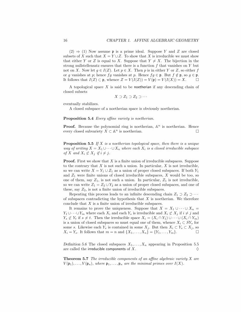
16 CHAPTER 1. AFFINE ALGEBRAIC GEOMETRY
(2) ⇒ (1) Now assume p is a prime ideal. Suppose Y and Z are closedsubsets of X such that X = Y ∪Z. To show that X is irreducible we must showthat either Y or Z is equal to X. Suppose that Y 6= X. The bijection in thestrong nullstellensatz ensures that there is a function f that vanishes on Y butnot on X. Now let g ∈ I(Z). Let p ∈ X. Then p is in either Y or Z, so either for g vanishes at p; hence fg vanishes at p. Hence fg ∈ p. But f /∈ p, so g ∈ p.It follows that I(Z) ⊂ p, whence Z = V (I(Z)) = V (p) = V (I(X)) = X.
A topological space X is said to be noetherian if any descending chain ofclosed subsets
X ⊃ Z1 ⊃ Z2 ⊃ · · ·
eventually stabilizes.A closed subspace of a noetherian space is obviously noetherian.
Proposition 5.4 Every affine variety is noetherian.
Proof. Because the polynomial ring is noetherian, An is noetherian. Henceevery closed subvariety X ⊂ An is noetherian.
Proposition 5.5 If X is a noetherian topological space, then there is a uniqueway of writing X = X1∪ · · ·∪Xn where each Xi is a closed irreducible subspaceof X and Xi 6⊂ Xj if i 6= j.
Proof. First we show that X is a finite union of irreducible subspaces. Supposeto the contrary that X is not such a union. In particular, X is not irreducible,so we can write X = Y1 ∪ Z1 as a union of proper closed subspaces. If both Y1
and Z1 were finite unions of closed irreducible subspaces, X would be too, soone of them, say Z1, is not such a union. In particular, Z1 is not irreducible,so we can write Z1 = Z2 ∪ Y2 as a union of proper closed subspaces, and one ofthese, say Z2, is not a finite union of irreducible subspaces.
Repeating this process leads to an infinite descending chain Z1 ⊃ Z2 ⊃ · · ·of subspaces contradicting the hypothesis that X is noetherian. We thereforeconclude that X is a finite union of irreducible subspaces.
It remains to prove the uniqueness. Suppose that X = X1 ∪ · · · ∪ Xn =Y1 ∪ · · · ∪Ym where each Xi and each Ys is irreducible and Xi 6⊂ Xj if i 6= j andYs 6⊂ Yt if s 6= t. Then the irreducible space Xi = (Xi ∩ Y1) ∪ · · · ∪ (Xi ∩ Ym)is a union of closed subspaces so must equal one of them, whence Xi ⊂ SYs forsome s. Likewise each Ys is contained in some Xj . But then Xi ⊂ Ys ⊂ Xj , soXi = Ys. It follows that m = n and X1, . . . , Xn = Y1, . . . , Ym.
Definition 5.6 The closed subspaces X1, . . . , Xn appearing in Proposition 5.5are called the irreducible components of X. ♦
Theorem 5.7 The irreducible components of an affine algebraic variety X areV (p1), . . . , V (pn), where p1, . . . , pn are the minimal primes over I(X).

1.5. IRREDUCIBLE AFFINE VARIETIES 17
Proof. We can view X as a closed subvariety of some affine space Am. LetI(X) be the ideal of functions vanishing on X. Let p1, . . . , pn be the distinctminimal primes over X. Since I(X) is radical, I(X) = p1 ∩ · · · ∩ pn, whence
X = V (p1 ∩ · · · ∩ pn) = V (p1) ∪ · · · ∪ V (pn).
Now Xi := V (pi) is a closed irreducible subvariety of X, and because pj 6⊂ piwhen i 6= j, Xi 6⊂ Xj when i 6= j.
The minimal primes over a principal ideal fR in a UFD R are p1R, . . . , pnRwhere p1, . . . , pn are the distinct irreducible divisors of f . Hence the irreduciblecomponents of V (f) are V (p1), . . . , V (pn). Expressing a variety as the union ofits irreducible components is the geometric analog of expressing an element asa product of powers of irreducibles.
Theorem 5.7 suggests that we can examine an algebraic variety by study-ing one irreducible component at a time. This is why, in algebraic geometrytexts, you will often see the hypothesis that the variety under considerationis irreducible. Of course, questions such as how do the irreducible componentsintersect one another cannot be studied one component at a time.
Lemma 5.8 Let X be a subspace of a topological space Y . Then every irre-ducible component of X is contained in an irreducible component of Y .
Proof. Let Z be an irreducible component of X. Write Y = ∪i∈IYi wherethe Yis are the distinct irreducible components of Y . Then Z = ∪i∈I(Z ∩ Yi)expresses Z as a union of closed subspaces. But Z is irreducible so some Z ∩ Yiis equal to Z; i.e., Z ⊂ Yi for some i.
Lemma 5.9 Let f : X → Y be a continuous map between topological spaces.Then
1. if X is irreducible so is f(X);
2. if Z is an irreducible component of X, then f(Z) is contained in an irre-ducible component of Y .
Proof. (1) We can, and do, replace Y by f(X) and f(X) is given the sub-space topology. If f(X) = W1 ∪ W2 with each Wi closed in f(X), thenX = f−1(f(X)) = f−1(W1) ∪ f−1(W2) so X = f−1(Wi) for some i. Thusf(X) ⊂Wi. Hence f(X) is irreducible.
(2) Let Z be an irreducible component of X. By (1), f(Z) is an irreduciblesubspace of Y so, by Lemma 5.8, f(Z) is contained in an irreducible componentof Y .
Connected components and idempotents. A topological space X isconnected if the only way in which it can be written as a disjoint union of closedsubsets X = X1tX2 is if one of those sets is equal to X and the other is empty.There is a unique way of writing X as a disjoint union of connected subspaces,and those subspaces are called the connected components of X.

18 CHAPTER 1. AFFINE ALGEBRAIC GEOMETRY
An affine algebraic variety has only finitely many connected componentsbecause it is noetherian.
An irreducible variety is connected, but the converse is not true: for exam-ple, the union of the axes V (xy) ⊂ A2 is conncted but not irreducible. Hencethe decomposition of a variety into its connected components is a coarser de-composition than that into its irreducible components.
Suppose a variety X is not connected and write X = X1 tX2 with X1 6= φand X2 6= φ. Write Ij = I(Xj). Then I1 ∩ I2 = 0 because X1 ∪ X2 = X,and I1 + I2 = R because X1 ∩X2 = φ. In other words, we have a direct sumdecomposition O(X) = I1⊕ I2. Conversely, if O(X) = I⊕J is a decompositionas a direct sum of two non-zero ideals, there is a non-trivial decompositionX = V (I) t V (J).
If O(X) = I1 ⊕ I2 there is a unique way of writing 1 = e1 + e2 with ej ∈ Ij .It is clear that e1 and e2 are orthogonal idempotents, i.e., e2j = ej and e1e2 =e2e1 = 0. Notice that e1 is the function that is identically 1 on X2 and zero onX1.
More generally, a decomposition X = X1 t · · · tXn into connected compo-nents corresponds to a decomposition 1 = e1 + · · ·+en of 1 as a sum of pairwiseorthogonal idempotents.
1.6 Plane Curves
The simplest algebraic varieties after those consisting of a finite set of pointsare the plane curves. These have been of central importance in mathematicssince ancient times. Earlier we defined a plane curve as V (f) where f ∈ k[x, y]is a non-constant polynomial (see Example 1.2) and showed that a plane curvehas infinitely many points when k is algebraically closed. In this section we willshow that the intersection of two distinct irreducible curves is a finite set.
We continue to work over an algebraically closed field k.
Lemma 6.1 Let R be a UFD and 0 6= f, g ∈ R[X]. Then f and g have acommon factor of degree ≥ 1 if and only if af = bg for some non-zero a, b ∈ R[x]such that deg a < deg g (equivalently deg b < deg f).
Proof. (⇒) If f = bc and g = ac where c is a common factor of degree ≥ 1,the af = bg and deg a < deg g.
(⇐) Suppose such a and b exist. Because R[X] is a UFD we can cancel anycommon factors of a and b, so we will assume that a and b have no commonfactor. Since R[X] is a UFD and a|bg it follows that a|g. Thus g = ac anddeg c > 0 since deg a < deg g. Now af = bg = bac implies f = bc so c is acommon factor.
Definition 6.2 Let R be a domain. The resultant, R(f, g), of polynomials
f = a0Xm + . . .+ am−1X + am
g = b0Xn + . . .+ bn−1X + bn

1.6. PLANE CURVES 19
in R[X] of degrees m and n is the determinant of the (m+n)× (m+n) matrix
a0 a1 . . . am 0 . . . 00 a0 a1 . . . am 0 . . . 0...
...b0 b1 . . . bn−1 bn 0 . . . 00 b0 b1 . . . bn−1 bn 0 . . . 0...
...0 . . . 0 b0 b1 . . . bn−1 bn
where there are n rows of the a’s and m rows of the b’s. ♦
Lemma 6.3 Let R be a UFD and 0 6= f, g ∈ R[X]. Then f and g have acommon factor of degree ≥ 1 if and only if R(f, g) = 0.
Proof. By Lemma 6.1 it suffices to show that R(f, g) = 0 if and only if af = bgfor some 0 6= a, b ∈ R[X] such that deg a < deg g and deg b < deg f . It imposesno additional restriction to require that deg a = deg g−1 and deg b = deg f −1.There exist such polynomials
a =n−1∑i=0
ciXn−1−i and b = −
m−1∑j=0
djXm−1−j
if and only if
(c0Xn−1 + c1Xn−2 + · · ·+ cn−2X + cn−1)(a0X
m + · · ·+ am−1X + am) +
(d0Xm−1 + d1X
m−2 + · · ·+ dm−2X + dm−1)(b0Xn + · · ·+ bn−1X + bn) = 0.
Thus f and g have a common factor if and only if there is a solution to thematrix equation
a0 a1 . . . am 0 . . . 00 a0 a1 . . . am 0 . . . 0...
...b0 b1 . . . bn−1 bn 0 . . . 00 b0 b1 . . . bn−1 bn 0 . . . 0...
...0 . . . 0 b0 b1 . . . bn−1 bn
cn−1
cn−2
...c0
dm−1
...d0
= 0;
i.e., if and only if R(f, g) = 0.
Proposition 6.4 Let f, g ∈ R[X]. Then R(f, g) = cf+dg for some c, d ∈ R[X]with deg c = deg g − 1 and deg d = deg f − 1. In particular, R(f, g) belongs tothe ideal (f, g).

20 CHAPTER 1. AFFINE ALGEBRAIC GEOMETRY
Proof. For each i = 1, . . . ,m+ n multiply the ith column of the matrix whosedeterminant is R(f, g) by Xm+n−i and add it to the last column. This leavesall columns unchanged except the last which is now the transpose of(
Xn−1f Xn−2f . . . Xf f Xm−1g Xm−2g . . . Xg g).
The determinant of this new matrix is the same as the determinant of theoriginal one, namely R(f, g). But computing the determinant by expandingthis new matrix down the last column shows that R(f, g) = cf + dg.
Corollary 6.5 Let f, g ∈ k[x, y] be polynomials of positive degree having nocommon factor. Then V (f, g) is finite.
Proof. Let I be the ideal of k[x, y] generated by f and g.First view f and g as polynomials in R[x] where R = k[y]. Because f and
g have no common factor R(f, g) 6= 0. But R(f, g) ∈ k[y] and is also in I byProposition 6.4. Hence I ∩ k[y] 6= 0. Similarly, I ∩ k[x] 6= 0.
Let 0 6= a ∈ I ∩ k[y] and 0 6= b ∈ I ∩ k[x]. Then V (f, g) ⊂ V (a, b) =V (a) ∩ V (b). But V (a) is a finite union of horizontal lines λ × A1 where λruns over the zeroes of a ∈ k[y]. Similarly, V (b) is a finite union of vertical lines,so V (a) ∩ V (b) is finite. It follows that V (f, g) is finite.
Corollary 6.6 Let k be an algebraically closed field, and let f, g ∈ k[x] bepolynomials of degree m and n respectively. Then f and g have a common zeroif and only if R(f, g) = 0.
Proof. If they have a common zero, say λ ∈ k then they have the commonfactor (x − λ), so R(f, g) = 0. Conversely, if R(f, g) = 0 then they have acommon factor, and hence a common factor of degree 1, say x − λ, since k isalgebraically closed. Thus f(λ) = g(λ) = 0.
The next result gives a more concrete interpretation of the resultant R(f, g):it is the determinant of a map which is rather naturally defined in terms of f andg. Before we state the result, recall that if R is a commutative ring, N a free R-module, and ϕ : N → N a R-module map, then a choice of basis for N allows usto express ϕ as a matrix with respect to that basis, and the determinant of thatmatrix may be defined in the usual way. Since the determinant is independentof the choice of basis, we may speak of the determinant of ϕ, det(ϕ), as awell-defined element of R.
Theorem 6.7 Let R be a domain and suppose that f =∑mi=0 aiX
m−i andg =
∑ni=0 biX
n−i are polynomials in R[X] such that a0 and b0 are units in R.Then R[X]/(f) is a free R-module of rank m, and if ϕ : R[X]/(f)→ R[X]/(f)is defined by ϕ(a) = ga, then
det(ϕ) = cR(f, g)for some unit c ∈ R.

1.6. PLANE CURVES 21
Proof. The proof is given in several steps, and is finally completed by combiningsteps (2) and (7). For each j ≥ 1 define Vj = R⊕RX ⊕ . . .⊕RXj−1.
Step 1 Claim: R[X] = (f) ⊕ Vm. Proof: Since deg(f) = m, (f) ∩ Vm = 0.The R-module (f) + Vm contains 1, X, . . . ,Xm−1 and also Xm since a0 is aunit. Therefore, if Xj = fa+ b with b ∈ Vm then Xj+1 = faX + bX is also in(f) + Vm. The result follows by induction on j.
Step 2 It follows that the natural map γ : Vm → R[X] → R[X]/(f) is a R-module isomorphism. Define ψ : Vm → Vm by ψ = γ−1ϕγ. Then det(ψ) =det(ϕ).
Step 3 Claim: if w ∈ Vm, then there is a unique v ∈ Vn such that fv+ gw ∈Vm. Proof: Since R[X] = (f)⊕Vm, and since R[X] is a domain, there is a uniquev ∈ R[X] such that fv + gw ∈ Vm. Now deg(fv) ≤ maxdeg(gw),m − 1 ≤m+ n− 1, so deg(v) ≤ n− 1 as required.
Step 4 For each w ∈ Vm define θ(w) = Xmv where v ∈ Vn has the propertyfv + gw ∈ Vm. The uniqueness of v ensures that we obtain a well-defined mapθ : Vm → XmVn. It is routine to check that θ is a R-module homomorphism.
Step 5 Claim: R(f, g) = det(ρ) where ρ : Vm+n = XmVn⊕Vm → Vm+n is de-fined by ρ(Xmv+w) = fv+gw for v ∈ Vn, w ∈ Vm. Proof: Consider the matrixrepresentation of ρ with respect to the ordered basisXm+n−1, Xm+n−2, . . . , X, 1for the free R-module Vm+n. We have
ρ(Xm+n−1) = fXn−1 = a0Xm+n−1 + a1X
m+n−2 + . . .+ amXn−1
ρ(Xm+n−2) = fXn−2 = a0Xm+n−2 + a1X
m+n−3 + . . .+ amXn−2
...ρ(Xm) = f = a0X
m + . . .+ am
ρ(Xm−1) = gXm−1 = b0Xm+n−1 + b1X
m+n−2 + . . .+ bnXm−1
...
ρ(1) = g = b0Xn−1 + . . .+ bn
Thus the matrix representing ρ is
a0 0 . . . 0 b0 0 . . . 00 a0 . . . 0 b1 b0 . . . 0...
......
......
am am−1 . . . . . . 00 am . . . . . . 0...
......
......
0 0 . . . a0 bn−1 . . .0 0 . . . a1 bn bn−1 . . .0 0 . . . a2 0 bn . . ....
......
......
0 0 . . . am 0 0 . . . bn

22 CHAPTER 1. AFFINE ALGEBRAIC GEOMETRY
which is the transpose of the matrix whose determinant is R(f, g). Hencedet(ρ) = R(f, g).
Step 6 Claim: ψ = ρ(θ + 1) on Vm. Proof: Let w ∈ Vm. Thenγρ(θ + 1)(w) = γρ(θ(w) + w) = γ(fX−mθ(w) + gw) = γ(gw) = gγ(w) = ϕγ(w)whence γρ(θ + 1) = ϕγ. The claim follows since ψ = γ−1ϕγ.
Step 7 Claim: There is a unit c ∈ R such that det(ρ) = cdet(ψ). Proof: Ifu ∈ XmVn and w ∈ Vm, we will write the element u+w ∈ Vm+n = XmVn⊕Vmas a column vector
(uw
). We will also represent a R-module map Vm+n → Vm+n
as a blocked matrix accordingly. For example, ρ =(ρ11 ρ12
ρ21 ρ22
)where ρ11 :
XmVn → XmVn, ρ12 : Vm → XmVn etc. In particular(ρ11 0ρ21 IdVm
)(uw
)=(
ρ11(u)ρ21(u) + w
)= ρ11(u) + ρ21(u) + w = ρ(u) + w.
Thus (ρ11 0ρ21 IdVm
)(IdXmVn
−θ0 ψ
)(uw
)=(ρ11 0ρ21 IdVm
)(u− θ(w)ψ(w)
)= ρ(u− θ(w)) + ψ(w)= ρ(u) + ρ(w).
Thus (ρ11 0ρ21 1
)(1 −θ0 ψ
)= ρ,
from which it follows that det(ρ) = det(ρ11) det(ψ).It remains to show that ρ11 is invertible, and hence that det(ρ11) is a unit
in R. By definition, if v ∈ Vn then ρ11(Xmv) is the component of ρ(Xmv) = fvin XmVn. Since fVn ∩ Vm = 0, ρ11 is injective. On the other hand, ρ11 is aR-module map, so it is enough to show that Xm, Xm+1, . . . , Xm+n−1 are in theimage of ρ11. Now ρ11(Xm) is the component of f in XmVn, namely a0X
m.Since a0 is a unit, Xm ∈ Im(ρ11). Now ρ11(Xm+1) = a0X
m+1 + a1Xm, and
since Xm ∈ Im(ρ11) we have Xm+1 ∈ Im(ρ11). Continuing inductively yieldsthe result.
1.7 Morphisms between affine varieties
Algebraic geometry is the study of algebraic varieties and the maps betweenthem.
Our next job is to specify the class of maps we allow between two affinealgebraic varieties; i.e., what maps ψ : X → Y should we allow between closedsubvarieties X ⊂ An and Y ⊂ Am? We will eventually call the allowable mapsbetween two varieties morphisms, so the question is, what are the morphismsψ : X → Y between two affine algebraic varieties?
The answer appears in Definition 7.1 below, but let’s take our time gettingthere and see why that definition is reasonable.
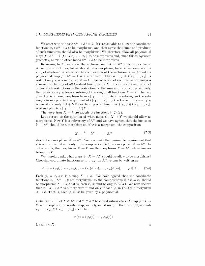
1.7. MORPHISMS BETWEEN AFFINE VARIETIES 23
We start with the case An → A1 = k. It is reasonable to allow the coordinatefunctions xi : An → k to be morphisms, and then agree that sums and productsof such functions should also be morphisms. We therefore allow all polynomialmaps f : An → k, f ∈ k[x1, . . . , xn], to be morphisms and, since this is algebraicgeometry, allow no other maps An → k to be morphisms.
Returning to X, we allow the inclusion map X → An to be a morphism.A composition of morphisms should be a morphism, because we want a cate-gory of algebraic varieties, so the composition of the inclusion X → An with apolynomial map f : An → k is a morphism. That is, if f ∈ k[x1, . . . , xn] itsrestriction f |X is a morphism X → k. The collection of such restriction maps isa subset of the ring of all k-valued functions on X. Since the sum and productof two such restrictions is the restriction of the sum and product respectively,the restrictions f |X form a subring of the ring of all functions X → k. The rulef 7→ f |X is a homomorphism from k[x1, . . . , xn] onto this subring, so the sub-ring is isomorphic to the quotient of k[x1, . . . , xn] by the kernel. However, f |Xis zero if and only if f ∈ I(X) so the ring of all functions f |X , f ∈ k[x1, . . . , xn],is isomorphic to k[x1, . . . , xn]/I(X).
The morphisms X → k are exactly the functions in O(X).Let’s return to the question of what maps ψ : X → Y we should allow as
morphisms. Now Y is a subvariety of Am and we have agreed that the inclusionY → Am should be a morphism so, if ψ is a morphism, the composition
Xψ−−−−→ Y −−−−→ Am (7-3)
should be a morphism X → Am. We now make the reasonable requirement thatψ is a morphism if and only if the composition (7-3) is a morphism X → Am. Inother words, the morphisms X → Y are the morphisms X → Am whose imagesbelong to Y .
We therefore ask, what maps ψ : X → Am should we allow to be morphisms?Choosing coordinate functions x1, . . . , xm on Am, ψ can be written as
ψ(p) = (ψ1(p), · · · , ψm(p)) = (x1(ψ(p)), . . . , xm(ψ(p)), p ∈ X. (7-4)
Each ψi = xi ψ is a map X → k. We have agreed that the coordinatefunctions xi : Am → k are morphisms, so the compositions xi ψ = ψi shouldbe morphisms X → k; that is, each ψi should belong to O(X). We now declarethat ψ : X → Am is a morphism if and only if each ψi in (7-4) is a morphismX → k. That is, each ψi must be given by a polynomial.
Definition 7.1 Let X ⊂ An and Y ⊂ Am be closed subvarieties. A map ψ : X →Y is a morphism, or regular map, or polynomial map, if there are polynomialsψ1, . . . , ψm ∈ k[x1, . . . , xn] such that
ψ(p) = (ψ1(p), · · · , ψm(p))
for all p ∈ X. ♦
24 CHAPTER 1. AFFINE ALGEBRAIC GEOMETRY
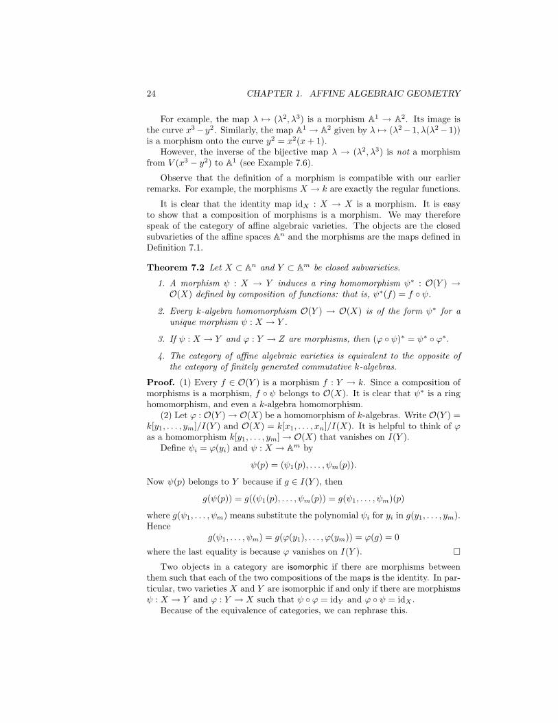
For example, the map λ 7→ (λ2, λ3) is a morphism A1 → A2. Its image isthe curve x3− y2. Similarly, the map A1 → A2 given by λ 7→ (λ2− 1, λ(λ2− 1))is a morphism onto the curve y2 = x2(x+ 1).
However, the inverse of the bijective map λ → (λ2, λ3) is not a morphismfrom V (x3 − y2) to A1 (see Example 7.6).
Observe that the definition of a morphism is compatible with our earlierremarks. For example, the morphisms X → k are exactly the regular functions.
It is clear that the identity map idX : X → X is a morphism. It is easyto show that a composition of morphisms is a morphism. We may thereforespeak of the category of affine algebraic varieties. The objects are the closedsubvarieties of the affine spaces An and the morphisms are the maps defined inDefinition 7.1.
Theorem 7.2 Let X ⊂ An and Y ⊂ Am be closed subvarieties.
1. A morphism ψ : X → Y induces a ring homomorphism ψ∗ : O(Y ) →O(X) defined by composition of functions: that is, ψ∗(f) = f ψ.
2. Every k-algebra homomorphism O(Y ) → O(X) is of the form ψ∗ for aunique morphism ψ : X → Y .
3. If ψ : X → Y and ϕ : Y → Z are morphisms, then (ϕ ψ)∗ = ψ∗ ϕ∗.
4. The category of affine algebraic varieties is equivalent to the opposite ofthe category of finitely generated commutative k-algebras.
Proof. (1) Every f ∈ O(Y ) is a morphism f : Y → k. Since a composition ofmorphisms is a morphism, f ψ belongs to O(X). It is clear that ψ∗ is a ringhomomorphism, and even a k-algebra homomorphism.
(2) Let ϕ : O(Y )→ O(X) be a homomorphism of k-algebras. Write O(Y ) =k[y1, . . . , ym]/I(Y ) and O(X) = k[x1, . . . , xn]/I(X). It is helpful to think of ϕas a homomorphism k[y1, . . . , ym]→ O(X) that vanishes on I(Y ).
Define ψi = ϕ(yi) and ψ : X → Am by
ψ(p) = (ψ1(p), . . . , ψm(p)).
Now ψ(p) belongs to Y because if g ∈ I(Y ), then
g(ψ(p)) = g((ψ1(p), . . . , ψm(p)) = g(ψ1, . . . , ψm)(p)
where g(ψ1, . . . , ψm) means substitute the polynomial ψi for yi in g(y1, . . . , ym).Hence
g(ψ1, . . . , ψm) = g(ϕ(y1), . . . , ϕ(ym)) = ϕ(g) = 0
where the last equality is because ϕ vanishes on I(Y ).
Two objects in a category are isomorphic if there are morphisms betweenthem such that each of the two compositions of the maps is the identity. In par-ticular, two varieties X and Y are isomorphic if and only if there are morphismsψ : X → Y and ϕ : Y → X such that ψ ϕ = idY and ϕ ψ = idX .
Because of the equivalence of categories, we can rephrase this.

1.7. MORPHISMS BETWEEN AFFINE VARIETIES 25
Proposition 7.3 Two affine varieties X and Y are isomorphic if and only ifthe k-algebras O(X) and O(Y ) are isomorphic.
Corollary 7.4 If X and Y are finite affine varieties, then X ∼= Y if and onlyif |X| = |Y |.
Proof. (⇒) This is obvious.(⇐) By the remarks after Lemma 2.4, O(X) is equal to the ring of all
functions X → k. This ring obviously depends only on the cardinality of X.Hence the result.
Remark. If X and Y are finite varieties then any set map X → Y is amorphism (because any map X → k is a regular function). Suppose that G isa finite group. Then we can view G as an affine variety, and the mutiplicationmap G×G→ G and the inversion G→ G, g 7→ g1 , are morphisms. In this wayG becomes an algebraic group (see later).
Example 7.5 Let f(x) ∈ k[x] be any non-zero polynomial. Then the curvey = f(x) is isomorphic to the affine line via the morphism t 7→ (t, f(t)) and itsinverse (x, y) 7→ x. Equivalently, the k-algebra homomorphism φ : k[x, y]→ k[x]given by φ(x) = x and φ(y) = f(x) is surjective and has kernel (y − f(x)). ♦
Example 7.6 Not every continuous map between affine varieties is a morphism.1. Recall that the closed subsets of A1 are just the finite subsets and A1
itself. It follows that every bijective set map A1 → A1 is continuous in theZariski topology. No doubt you can think of lots of bijective maps C→ C thatare not given by polynomial maps.
2. The map ψ−1 : X → A1 that is the inverse of the morphism λ 7→ (λ2, λ3)to the cusp X = V (y2−x3), is bijective, hence continuous. But ψ−1 is not givenby the restriction of a polynomial map A2 → k so is not a morphism. To verifythis last claim, suppose to the contrary that ψ−1 is given by a polynomial f ∈k[x, y]; i.e., f |C = ψ−1. In particular, if λ 6= 0, then f(λ2, λ3) = ψ−1(λ2, λ3) =λ; in other words, λ3f(λ2, λ3) = λ2. Hence yf − x vanishes at (λ2, λ3).
Now V (yf − x) is closed in A2 and contains C\0, so contains C. Sinceyf − x vanishes on C it is a multiple of y2 − x3. Passing to k[x, y]/(y2 − x3)which is isomorphic to k[t2, t3], this gives t3f = t2. That is not possible!
3. The Frobenius morphism. If char k = p, the map f 7→ fp from k[x1, . . . , xn]to itself is a ring homomorphism. The corresponding morphism Fr : An → An,(a1, . . . , an) → (ap1, . . . , a
pn) is called the Frobenius morphism. It is bijective,
hence a homeomorphism, but its inverse is not a morphism. ♦
Exercise. Let f : X → Y be a morphism. If X ′ is an irreducible componentof X show that f(X ′) is contained in one of the irreducible components of Y .
Proposition 7.7 Let f : X → Y be a morphism between affine varieties andwrite φ : O(Y )→ O(X) for the corresponding ring homomorphism. Then
1. if Z ⊂ Y is closed, then f−1(Z) = V (φ(I(Z)));

26 CHAPTER 1. AFFINE ALGEBRAIC GEOMETRY
2. f is continuous,
3. if W ⊂ X is closed, then I(f(W )) = φ−1(I(W )) = I(f(W ));
4. kerφ = I(f(X)) and f(X) = V (kerφ);
5. φ is injective if and only if f(X) is dense in Y ;
6. the fibers Xy := f−1(y) are closed subvarieties of X;
7. mf(x) = φ−1(mx).
Proof. (1) Let J = I(Z). Then
f−1(Z) = x ∈ X | f(x) ∈ Z= x ∈ X | g(f(x)) = 0 for all g ∈ J= x ∈ X | φ(g)(x) = 0 for all g ∈ J= V (φ(J)).
(2) Part (1) shows that the inverse image of a closed set is closed, so f iscontinuous.
(3) We have
I(f(W )) = g ∈ O(Y ) | g(f(W )) = 0= g ∈ O(Y ) | φ(g)(W ) = 0= g ∈ O(Y ) | φ(g) ∈ I(W )= φ−1(I(W )).
(4) Applying (3) with W = X gives
kerφ = φ−1(0) = φ−1(I(X)) = I(f(X)).
By Lemma 1.7, f(X) = V (I(f(X)) = V (kerφ).(5) This follows from (4).(6) and (7) are special cases of (1) and (3) respectively.
A morphism f : X → Y need not send closed sets to closed sets. Forexample, the projection of the hyperbola xy = 1 onto the x-axis is a morphismand the image of the hyperbola is A1 − 0.
Lemma 7.8 If f : X → Y is a continuous map between topological spacesand X is irreducible, then both f(X) and f(X) are irreducible (when given thesubspace topology).
Proof. Suppose f(X) = Z ∪W where Z and W are closed subspaces of f(X).Then X = f−1(Z)∪ f−1(W ) expresses X as a union of closed subspaces so oneof them equals X, say X = f−1(Z). Then f(X) = Z, so f(X) is irreducible.

1.7. MORPHISMS BETWEEN AFFINE VARIETIES 27
We will now show that if U is any subspace of Y that is irreducible (withthe induced subspace topology), then U is irreducible. The Lemma will followwhen we apply this to U = f(X).
If U = Z ∪W , then U = (U ∩Z)∪ (U ∩W ) expresses U as a union of closedsubspaces of itself; hence U is equal to either U ∩Z or U ∩W , and either U ⊂ Zor U ⊂ W , whence U is contained in either Z or W , and so equal to either Zor W . Hence U is irreducible.
Dominant morphisms. When considering a continuous map f : X → Ybetween topological spaces one can frequently replace Y by f(X) and considerinstead the surjective map f : X → f(X). We can’t quite do this when consid-ering morphisms between varieties because f(X) need not be an affine variety—the problem is that f(X) need not be a closed subspace of Y . However, we canreplace Y by f(X) and then consider the morphism f : X → f(X) betweenvarieties.
Definition 7.9 A morphism f : X → Y is dominant if f(X) = Y , i.e., if theimage of f is dense in Y . ♦
Part (5) of Proposition 7.7 says that f : X → Y is dominant if and only ifthe corresponding k-agebra homomorphism φ : O(Y )→ O(X) is injective. Thehypothesis that a morphism is dominant is the geometric analogue of the hy-pothesis that a ring homomorphism is injective; or, it is the geometric analogueof “subalgebra”.
Part (2) of Lemma 7.8 allows us to restrict our attention to morphismsbetween irreducible algebraic varieties.
The next example further reinforces the idea that dominance rather thansurjectivity is the key notion for morphisms.
Example 7.10 There exists a surjective morphism f : X → Y in which Y isirreducible but f |Z : Z → Y is not surjective for any irreducible component Zof X.
Take X = V (x(xy − 1)) ⊂ A2; then X = L∪C where L is the y-axis and Cis the hyperbola y = x−1, and these are the two irreducible components of X.Now let Y = A1 be the x-axis and f : X → Y the projection onto the x-axis;i.e., f(x, y) = x. Then Y is irreducible and f is surjective, but f(L) = 0 andf(C) = Y − 0, so neither f |L nor f |C is surjective. ♦
The function field of an irreducible variety. Let X be an irreducibleaffine variety over k. Then O(X) is a domain. We usually write k(X) for thefield of fractions of O(X) and call it the function field or the field of rationalfunctions on X.
Let f : X → Y be a dominant morphism between irreducible varieties. ThenO(X) is a domain and, since the homomorphism φ : O(Y )→ O(X) is injective,

28 CHAPTER 1. AFFINE ALGEBRAIC GEOMETRY
there is a commutative diagram of inclusions
O(Y ) −−−−→ k(Y )y yO(X) −−−−→ k(X).
We therefore view k(Y ) and a subfield of k(X).Let X be an irreducible algebraic variety and f ∈ k(X). Write f = g/h
where g, h ∈ O(X). We can evaluate f at those points x ∈ X such thath(x) 6= 0. We usually write
Xh := x ∈ X | h(x) 6= 0.
This is an open subset of X because the zero locus of h is closed. Also, if h isnot zero Xh is a non-empty (see Remark 1 after Proposition 2.2) open subsetof X and hence dense. Thus f is defined on a dense open subset of X.
For example, the rational function f = x/z = z/y on the surface xy = z2 isdefined at all points except (0, 0, 0).
A finite intersection of dense open sets is dense and open so if we are given afinite number of non-zero regular functions on an irreducible X the locus wherenone of them vanishes is dense and open. Notice that an intersection of twodense subsets may be empty: for example the even (resp., odd) integers form adense subset of C in the Zariski topology, but their intersection is empty.
Final examples. Consider an affine algebraic variety X. By Lemma 2.4,there are enough functions inO(X) to distinguish the points, and more generallydisjoint closed subsets, of X. However, if x and y are different points of X thefunctions in k+ mxmy ⊂ O(X) no longer distinguish x and y: if f ∈ k+ mxmy,then f(x) = f(y). Now k + mxmy is a finitely generated k-subalgebra of O(X)so is the coordinate ring of some affine algebraic variety Y and the inclusionO(Y ) → O(X) corresponds to a morphism π : X → Y with the property thatπ(x) = π(y).
This is one crude way of constructing new varieties from old: by identifyingpoints.
Another simle example of this is to consider the subring k[x2] of k[x] =O(A1). Functions in k[x2] take the same value at the points p,−p ∈ A1. Thusk[x2] is the coordinate ring of A1/ ∼ where ∼ is the equivalence relation p ∼ −pon A1. Of course, A1/ ∼ is still an affine line, but it is a different affine linethan the original one.
One might be more ambitious and try to collapse a curve on a surface X toa single point. For example, if R = k[x, y], then a function in k + xR takes thesame value at all points of the y-axis V (x). However, k + xR is not a finitelygenerated k-algebra (because it is not noetherian–why?) so is not the coordinatering of an affine algebraic variety. However, the subalgebra k[x, xy] of k[x, y]is finitely generated and, because k[x, xy] ⊂ k + xR, a function in it takes thesame value at all points (0, ∗) ∈ A2. Precisely, k[x, xy] is also a polynomial ring

1.8. OPEN SUBSETS OF AN AFFINE VARIETY 29
in two variables so the inclusion k[x, xy] → k[x, y] corresponds to a morphismπ : A2 → A2 that sends the y-axis to the origin but is bijective elsewhere.
This example is also important because it shows that the fibers of a morphismcan have different dimensions.
The other reason this example is important is because it is the simplest(partial) example of blowing up a point on a surface. From the point of viewof the target X this map π : X = A2 → X = A2 has replaced the single point(0, 0) ∈ X by an affine line—we say we have blown up the origin.
Actually, blowing up a point on a surface really involves replacing the pointby a projective line P1. Over k = C, the projective line is the Riemann sphereCP1 so the point has been replaced by a sphere. Think of putting a straw intothe point and puffing, thus producing a bubble, the sphere CP1.
Returning to the idea of passing from O(X) to k+mxmy, one could considerinstead k+m2
x. This is also a finitely generated k-algebra so is of the form O(Y )and the inclusion O(Y ) ⊂ O(X) corresponds to a map π : X → Y . It is nothard to show that π is bijective (show that the map m 7→ m∩O(Y ) is a bijectionbetween the maximal ideals in O(X) and O(Y )). However, π : X → Y is notan isomorphism because one has lost some first order data. For example, lookat the case of X = A1 and the subring k[t2, t3] ⊂ k[t]. The map π : X → Yproduces a singularity at the origin.. For example, look at the case of X = A1
and the subring k[t2, t3] ⊂ k[t]. The map π : X → Y produces a singularity atthe origin.
1.8 Open subsets of an affine variety
We showed in section 1.2 that the topology on a closed subvariety X ⊂ Aninherited from the Zariski topology on An may be described intrinsically interms of O(X). Namely, the closed subsets of X are the
V (I) := x ∈ X | f(x) = 0 for all f ∈ O(X).
The simplest such sets are those of the form V (f), the zero loci of a singleequation f ∈ O(X). Their open complements
Xf := x ∈ X | f(x) 6= 0
are called basic open sets. They play a particularly important role. Notice thatXf ∩Xg = Xfg.
If Z ⊂ X is any closed set, say Z = x | f1(x) = · · · = fr(x) = 0, then
X − Z = Xf1 ∪Xf2 ∪ · · · ∪Xfr ,
so every open set is a finite union of basic open sets. In other words, the basicopen sets provide a basis for the Zariski topology on X.
Proposition 8.1 The open set Xf may be given the structure of an affine al-gebraic variety in such a way that the inclusion Xf → X is a morphism.

30 CHAPTER 1. AFFINE ALGEBRAIC GEOMETRY
Proof. Let I = I(X) be the ideal of X, x1, . . . , xn a set of coordinate functionson An, and let xn+1 be a new variable.. There is bijection
Xf ←→ V (I, fxn+1 − 1) ⊂ An+1
p←→ (p, f(p)−1) ∈ An × A1
so we will identify Xf with the closed subvariety V (I, fxn+1−1) of An+1. Doingthis we find
O(Xf ) =O(X)[xn+1](fxn+1 − 1)
= O(X)[f−1].
The projection map π : An+1 → An onto the first n coordinates yields a com-mutative diagram
V (I, fxn+1 − 1) −−−−→ An+1
i
y yπX = V (I) −−−−→ An
when restrictied to the indicated closed subvarieties. It is easy to see that iis a bijection onto Xf and is therefore a homeomorphism. The correspondingcommutative diagram of k-algebra homomorphisms is
O(X)[f−1] ←−−−− k[x1, . . . , xn, xn+1]x xO(X) ←−−−− k[x1, . . . , xn].
This completes the proof.
Remark. Not every open subset of X can be given the structure of analgebraic variety. For example, U = C2 − 0 can not be given the structure ofan algebraic variety in such a way that the inclusion U → C2 is a morphism.This is essentially because any regular function f : U → C would be regular onC − either axis so would belong to C[x, y][x−1] ∩ C[x, y][y−1] which is equalto C[x, y]. Thus the map O(C2)→ O(U) is an isomorphism, but this is absurdbecause of the Nullstellensatz—it would say that the natural map U → C2 is abijection.
Of course, C2 − 0 is not a pathological object so algebraic geometry mustbe adapted to accomodate it. This has been done long ago. What one does isthis. Rather than having a single ring of functions on C2−0, one has a sheafof functions on C2 − 0; that is, for every open subset U of C2 − 0 one hasa ring O(U) of C-valued functions, and there are some obvious compatibilitiesbetween these rings that correspond to inclusions U1 ⊂ U2 and so on. Thejargon is that C2 − 0 is a quasi-affine algebraic variety.
More generally, if X is an irreducible affine algebraic variety and Z is aclosed subvariety such that dimZ ≤ dimX − 2, then X − Z can not be giventhe structure of an affine algebraic variety.

1.8. OPEN SUBSETS OF AN AFFINE VARIETY 31
Exercise. Let f : X → Y be a morphism between two affine algebraic vari-eties and let φ : O(Y )→ O(X) be the corresponding k-algebra homomorphism.If g ∈ O(Y ), then f−1(Yg) = Xφ(g).
Birational Geometry. One of the long-standing themes in algebraic ge-ometry is birational geometry. Two irreducible varieties X and Y are birationalor birationally equivalent if k(X) ∼= k(Y ). A central problem in algebraic ge-ometry is to find, for a given variety X a nice variety Y that is birational toX. Of course one wants Y to be “nicer” than X in some way. For example,one might ask that Y be smooth. Of course, one can always do that becauseX has a dense open subset that is smooth, so one asks also that there be asurjective morphism f : Y → X with Y smooth and f an isomorphism on adense open set. Hironaka won the Fields Medal for proving that this is possiblein characteristic zero. You will win the Fields medal if you can prove the resultin positive charateristic.
The close relationship between a pair of birationally equivalent varieties isexhibited by the following observation.
Proposition 8.2 Two irreducible varieties are birational if and only if theypossess isomorphic dense open subvarieties.
Proof. Let X and Y be the irreducible varieties in question.(⇒) This is more straightforward than the proof suggests—the difficulty lies
in finding the domains of definition of the appropriate morphisms.Suppose φ : k(Y ) → k(X) is an isomorphism. Write O(Y ) = k[y1, . . . , ym]
and φ(yi) = aib−1i where ai, bi ∈ O(X). If we set b =
∏bi, then
φ(O(Y )) ⊂ O(X)[b−1].
In other words, if X ′ = Xb, the restriction of φ to O(Y ) corresponds to amorphism
f : X ′ → Y.
Similarly, there is a non-empty open subset Y ′ ⊂ Y such that restriction of φ−1
to O(X) corresponds to a morphism
g : Y ′ → X.
Define
X0 := f−1g−1(X ′) ⊂ X ′ and Y0 := g−1f−1(Y ′) ⊂ Y ′.
Because f is the morphism corresponding to an injective homomorphismO(Y )→O(X ′), f(X ′) is dense in Y ; thus Y ′ ∩ f(X ′) 6= φ and f−1(Y ′) 6= φ; repeatingthis argument we see that g−1f−1(Y ′) 6= φ also. Thus X0 and Y0 are non-emptyopen subvarieties of X and Y .
We now show that f(X0) ⊂ Y0 and g(Y0) ⊂ X0. We will prove the first ofthese inclusions; the same argument with the roles of X and Y reversed willthen establish the second inclusion.

32 CHAPTER 1. AFFINE ALGEBRAIC GEOMETRY
By definition, f(X0) ⊂ g−1(X ′). Let y ∈ g−1(X ′). Then y ∈ Y ′ and fg(y) ∈f(X ′). Because f and g are the morphisms corresponding to (restrictions of)φ and φ−1, fg(y) = y. Thus y ∈ g−1f−1(y) ⊂ g−1f−1(Y ′) = Y0. Hencef(X0) ⊂ g−1(X ′) ⊂ Y0. Similarly, g(Y0) ⊂ X0.
Now consider f and g as morphisms between X0 and Y0. Because these twomorphisms correspond to (restrictions of) φ and φ−1 it follows that fg = idY0
and gf = idX0 .(⇐) Let X0 ⊂ X and Y0 ⊂ Y be non-empty open subsets and f : X0 → Y0
an isomorphism. Then f induces an isomorphism O(Y0)→ O(X0) and extendsto an isomorphism k(Y0) → k(X0) between the fields of fractions. But theinclusions X0 → X and Y0 → Y also induce morphisms O(X) → O(X0) andO(Y )→ O(Y0) that extend to isomorphisms k(X)→ k(X0) and k(Y )→ k(Y0).All this can be expressed in the commutative diagram
O(Y ) −−−−→ O(X)y yO(Y0) −−−−→ O(X0)y y
k(Y ) = k(Y0) −−−−→ k(X0) = k(X).
This is long-winded. The point is simply thatX is birational to every non-emptyopen subvariety of itself.
In other words, birational varieties are almost isomorphic.
Theorem 8.3 Let X be an irreducible affine algebraic variety. Then X is bi-rational to a hypersurface.
Proof. (Characteristic zero.) Write K = k(X). We must show there is ahypersurface Y such that k(Y ) ∼= K.
Noether normalization provides a polynomial subalgebra S = k[x1, . . . , xd]over which O(X) is integral. Now K is a finite extension of F = FractS so thePrimitive Element Theorem tells us there is a single a ∈ K such that K = F (a).In other words, K ∼= F [T ]/(f) where f is the minimal polynomial of a. We canreplace f by any non-zero scalar multiple of itself so we can, and will, assumethat the coefficients of f belong to S.
Define Y ⊂ Ad+1 to be the zero locus of the polynomial f ∈ S[T ] =k[x1, . . . , xd, T ]. Thus Y is a hypersurface and there is a surjective map S[T ]→S[a], T 7→ a, whose kernel is (f) because f is the minimal polynomial of a overF . Thus O(Y ) ∼= S[a] and k(Y ) = FractO(Y ) ∼= FractS[a] = F (a) = K.
A further advantage of the birational perspective is that the study of fields isa branch of algebraic geometry. Given a finitely generated fieldK = k(x1, . . . , xn),there are many varieties having K as their function field. The geometric prop-erties of those varieties gives insight into the field K.

1.9. SOME ALGEBRA 33
For example, let K be a finite extension of C(x), the function field in onevariable. There is a unique smooth projective curve X having K as its functionfield. Not only is X an algebraic variety but it is also a compact Riemannsurface, and as such we can speak of its topological genus, the number of “holes”in it. The genus of X is then an invariant of the field K. The only smoothprojective curve of genus zero is the projective line P1, or CP1 if you prefer tothink of it as the Riemann sphere. Its function field is C(x). The affine line A1
Cis a dense open subvariety of P1.
The fields of genus one are of the form C(X) where X ⊂ C2 is the zero locusof a curve of the form y2 = x(x − 1)(x − λ) where λ 6= 0, 1. This is an opensubset of the plane projective curve Y 2Z = X(X − Z)(X − λZ).
1.9 Some algebra
Lemma 9.1 Let I be a finitely generated ideal in a domain R. If I 6= 0 andI 6= R, then I 6= I2.
Proof. Suppose I2 = I = x1R + · · · + xnR. Then there are elements aij ∈ Isuch that
xi = x1ai1 + · · ·+ xnain
for all i = 1, . . . , n. We can arrange this as a matrix equation
(x1 · · ·xn)M = 0
where M is the n× n matrix with entries
Mij =
aii − 1 if i = j
aij if i 6= j.
Notice that every non-diagonal element of M belongs to I and the product ofthe diagonal elements is of the form (−1)n + b with b ∈ I. It follows thatdetM = (−1)n + c with c ∈ I. However xM = 0 so detM = 0. Hence 1 ∈ I.
Theorem 9.2 (Krull’s Intersection Theorem) Let I be an ideal in a com-mutative noetherian ring R. If b ∈ ∩∞n=1I
n, then b ∈ bI. If I 6= R and R iseither a domain or local, then ∩∞n=1I
n = 0.
Proof. We may write I = a1R + · · · + atR. Since b ∈ In there is a ho-mogeneous polynomial Pn(X1, . . . , Xt) ∈ R[X1, . . . , Xt] of degree n such thatb = Pn(a1, . . . , at). Since R[X1, . . . , Xt] is noetherian there is an integer n suchthat Pn+1 is in the ideal generated by P1, . . . , Pn, say Pn+1 = Q1P1+· · ·+QnPn

34 CHAPTER 1. AFFINE ALGEBRAIC GEOMETRY
and each Qi is homomogeneous of degree ≥ 1. Hence
b = Pn+1(a1, . . . , at)
=n∑i=1
Qi(a1, . . . , at)Pi(a1, . . . , at)
= bn∑i=1
Qi(a1, . . . , at) ∈ bI.
Now suppose I 6= R. If R is a domain, then ∩∞n=1In = 0 because b = bx
with x ∈ I implies b = 0. If R is local, then b = bx implies b(1 − x) = 0 but1− x is a unit so b = 0.
The next result is already part of Theorem 4.6 but we state it again herebecause it is the key to the results on finite morphisms that appear in the nextsection. Also the proof we give now is the one usually appearing in commutativealgebra texts.
Proposition 9.3 Let R be a subring of S and suppose that S is a finitely gen-erated R-module. If m is a maximal ideal of R, then there is a maximal ideal nof S such that n ∩R = m.
Proof. We can write S =∑nj=1Rsj with s1 = 1.
First we show that S 6= Sm. Suppose to the contrary that S = Sm. ThenS =
∑sjRm =
∑sjm. For each i = 1, . . . , n, we may write si =
∑j rijsj for
suitable rij ∈ m. In other words,∑nj=1(δij − rij)sj = 0. Let M be the n × n
matrix with ijth entry δij−rij , set ∆ = detM and write s for the column vector(s1, . . . , sn)T. Thus Ms = 0, and
0 = (Madj)Ms = ∆s
where Madj is the adjoint matrix. Hence ∆si = 0 for all i; in particular,0 = ∆s1 = ∆ = det(δij − rij). Writing out this determinant explicitly we seethat 1 ∈ m. This is a contradiction, so we conclude that S 6= Sm.
Since Sm is a proper ideal of S it is contained in a maximal ideal, say n.Then n ∩R ⊃ m, and 1 /∈ n, so n ∩R = m because m is maximal.
1.10 Finite morphisms
Definition 10.1 A morphism f : X → Y between affine varieties X and Y isfinite if O(X) is a finitely generated O(Y )-module via the induced k-algebrahomomorphism φ : O(Y )→ O(X).
The degree of a finite surjective morphism f : X → Y between irreduciblevarieties is [k(X) : k(Y )] = dimk(Y ) k(X), the degree of the field extension. ♦

1.10. FINITE MORPHISMS 35
Remarks. The k-algebra homomorphism φ : O(Y )→ O(X) correspondingto a finite surjective morphism f : X → Y is injective by Proposition 7.7 so,when X and Y are irreducible, it induces an injective map k(Y )→ k(X). Hencethe definition of degree makes sense.
Theorem 10.2 Let f : X → Y be a finite dominant morphism. Suppose thatO(X) is generated by ≤ t elements as an O(Y )-module. Then
1. |f−1(y)| ≤ t for all y ∈ Y ;
2. f is surjective;
3. f sends closed sets to closed sets.
Proof. The hypothesis that f is dominant says that the corresponding k-algebrahomomorphism φ : O(Y )→ O(X) is injective, so we will simply view O(Y ) asa subalgebra of O(X).
(1) Let m be the maximal ideal of O(Y ) vanishing at y. Then f−1(y) =V (φ(m)). The morphism f−1(y)→ y induces a commutative diagram
O(Y )φ−−−−→ O(X)y y
O(Y )m = O(y) −−−−→ O(f−1(y)) = O(X)√
φ(m)O(X).
of k-algebra homomorphisms. Therefore O(f−1(y) is generated by ≤ t elementsas a module over O(y) ∼= k, i.e., O(f−1(y)) is a k-vector space of dimension≤ t. It now follows from Proposition 2.6 that f−1(y) is finite with cardinality≤ t.
(2) This is an immediate consequence of Proposition 9.3 because of thebijection between points and maximal ideals.
(3) Let W ⊂ X be closed. It suffices to show that f(W ) = f(W ). Therestriction f |W : W → f(W ) is a morphism of varieties. The correspondingk-algebra homomorphism fits into the commutative diagram
O(Y )φ−−−−→ O(X)y y
O(Y )I(f(W ) = O(f(W )) −−−−→ = O(X)
I(W ) = O(W ).
The bottom map is injective because I(f(W )) = φ−1(I(W )). Hence by (1)applied to f |W , f |W is a surjective morphism W → f(W ).
For example, the inclusion k[x2]→ k[x] makes k[x] a finitely generated k[x2]-module, generated by 1 and x for example, so the corresponding morphismψ : A1 → A1 is surjective with finite fibers. Explicitly, if λ ∈ A1, then
ψ−1(λ) =
0 if λ = 0±√λ if λ 6= 0
.

36 CHAPTER 1. AFFINE ALGEBRAIC GEOMETRY
Let Q be the surface over C cut out by xy = z2 in A3. Write u = 12 (x+ y) and
u = 12i (x−y). Then x = u+ iv and y = u− iv so the equation xy = z2 becomes
u2+v2 = z2. This makes it easier to picture the real surface as the doubly infiniteicecream cone with vertex at the origin. The map ψ : k[x, y, z]/(xy−z2)→ k[s, t]defined by x 7→ s2, y 7→ t2, and z 7→ st, makes k[s, t] a finitely generated O(Q)-module, generated by 1, s, t for example. The map ψ : A2 → Q, (s, t) 7→(s2, t2, st) is therefore surjective with finite fibers. What are the cardinalities ofthe fibers?
Example 10.3 Let f : A2 = X → A2 = Y be the morphism defined byf(x, y) = (xy, y). The corresponding k-algebra homomorphism φ : O(Y ) =k[s, t] → O(X) = k[x, y] is given by φ(s) = xy and φ(t) = y. It is better tothink of φ as the inclusion k[xy, y] → k[x, y]. The image of φ is (α, β) |β 6=0 ∪ (0, 0). It is clear that f(X) = Y . Notice that f−1((0, 0)) = (∗, 0) butfor every other point p = (α, β) ∈ f(X), f−1(p) = (αβ−1, β) is a singleton.In particular, we see that one of the fibers is a line and all other fibers aresingletons. Notice too that it now follows that k[x, y] is not a finitely generatedmodule over k[xy, y]. ♦
The upper bound on the cardinality of the fibers in Theorem 10.2 is far fromthe best possible result. We will now prove the definitive result: the cardinalityof the fibers is at most deg f .
First we show that deg f is no more than the number of generators for O(X)as a O(Y )-module.
Lemma 10.4 Let S be a domain with field of fractions L. Let R be a subring ofS and consider K = FractR as a subfield of L. If S is generated by t elementsas an R-module, then dimK L ≤ t and S contains a K-basis for L.
Proof. Suppose S = Rs1 + · · ·+Rst. Then Ks1 + · · ·+Kst is a subring of Lbecause
sisj ∈t∑
k=1
Rsk ⊂t∑
k=1
Ksk.
Now Ks1 + · · · + Kst is a domain and a finite dimensional K-vector space sois a field. But this field contains S so must equal L. It follows that L =Ks1 + · · · + Kst, and the result follows because some subset of s1, . . . , snmust provide a basis for L over K.
Exercise. In the situation of Lemma 10.4 show that a subset of L is linearlyindependent over K if and only if it is linearly independent over R.
Theorem 10.5 Let f : X → Y be a finite dominant morphism between irre-ducible varieties. Then the fibers of f have cardinality at most the degree of fand some fiber has that cardinality.

1.10. FINITE MORPHISMS 37
Proof. In order to lighten the notation we will write R = O(Y ) ⊂ S = O(X),K = k(Y ) ⊂ L = k(X), and n = deg f = [L : K]. There are inclusions
Y R −−−−→ K
f
x y yX S −−−−→ L.
By Lemma 10.4,L = Kf1 ⊕ · · · ⊕Kfn
for some f1, . . . , fn ∈ S. Without loss of generality we may assume that f1 = 1,so
R ⊂ Rf1 ⊕ · · · ⊕Rfn ⊂ S.
Consider the finitely generated R-module
M = S/(Rf1 ⊕ · · ·Rfn).
Let s ∈ S and write s for its image in M . Since s = a1f1 + · · · + anfn forsome ai ∈ K, there is a non-zero x ∈ R such that xs ∈ Rf1 + · · ·+Rfn. HenceAnn(s) 6= 0. NowM is a finitely generated R-module, sayM = Rm1+· · ·+Rmt,so AnnM = ∩ti=1 Ann(mi) and this is non-zero because a finite intersection ofnon-zero ideals in a domain is non-zero (look at their product!).
Write J = AnnM . Then Y − V (J) is non-empty and open, hence dense.Pick y ∈ Y − V (J) and let my be the maximal ideal of R vanishing at y. ThenJ + my = R. But
S
myS +Rf1 + · · ·+Rfn
is annihilated by my + J so must be zero. In other words, as an R-module, andthus as an R/my-module, S/myS is generated by the images of f1, . . . , fn. Thus
dimkS
myS≤ n = deg f.
Hence, as in the proof of Theorem 10.2, |f−1(y)| ≤ n.It remains to prove that this bound is obtained.
Noether normalization again. Let X be a closed subvariety of An. Thecoordinate ring O(X) is a finitely generated k-algebra, so Noether normalizationsays that O(X) contains a polynomial ring k[y1, . . . , ym] such that O(X) isintegral, and hence a finitely generated module, over k[y1, . . . , ym]. The inclusionk[y1, . . . , ym] → O(X) is a homomorphism of k-algebras, so corresponds to amorphism ψ : X → Am. By Corollary ??, ψ is surjective with finite fibers.
Let’s reconsider the example, k[t+t−1] ⊂ k[t, t−1]. Now, k[t, t−1] ∼= k[x, y]/(xy−1), so k[t, t−1] is isomorphic to the hyperbola xy = 1; let’s write X for thishyperbola. Since k[t + t−1] is the polynomial ring in one variable, it is thecoordinate ring of the affine line. Hence the inclusion k[t + t−1] → k[t, t−1]

38 CHAPTER 1. AFFINE ALGEBRAIC GEOMETRY
corresponds to a morphism X → A1. That morphism is given by (x, y) 7→ x+y,or (x, x−1) 7→ x + x−1. The surjectivity says that for every α ∈ k = A1, thereis a point (x, x−1) ∈ X such that x + x−1 = α; this is nothing more than thestatement that because k is algebraically closed the equation x2 + 1 = αx hasa solution in k. Because k[t, t−1] is generated by two elements as a k[t + t−1]-module, there are at most two points in each fiber ψ−1(α).
Contrast this with the inclusion k[t] ⊂ k[t, t−1]. The associated morphismX → A1 is given by (x, x−1) 7→ x. This morphism is not surjective (0 is notin the image). This tells us at once that k[t, t−1] is not a finitely generatedk[t]-module.
Example 10.6 Let R = k[t] and S = k[x, y] be the polynomial rings in one andtwo variables respectively. If φ : k[t]→ k[x, y] is any k-algebra homomorphism,then k[x, y] is not a finitely generated k[t]-module.
Proof: If kerφ 6= 0, then imφ has finite dimension so the infinite dimensionalvector space k[x, y] cannot be a finitely generated k[t]-module.
Now suppose φ is injective. The corresponding morphism f : A2 → A1 isthe map p 7→ φ(t)(p) so f−1(0) is the zero locus of the polynomial φ(t). ByTheorem 10.2 f−1(0) is finite; but Example 1.2 shows this can only happen ifφ(t) is a constant; but in that case φ is not injective. We conclude that there isno map φ making k[x, y] a finitely generated k[t]-module. ♦
1.11 Finite group actions
Let G ⊂ AutX be a finite group of automorphisms acting on a variety X. Let’swrite X/∼ for the set of orbits for the moment. One of the most importantconstructions in algebraic geometry is the imposition of an algebraic varietystructure on X/∼.
The strategy we employ to do this is not one you have met before. Sofar we have defined and/or constructed all varieties as explicit subvarieties ofparticular affine spaces. In contrast, we will first define a particular subringO(X)G ⊂ O(X), then show there is a variety having O(X)G as its coordinatering, then introduce the notation X/G for that variety. We do not know whatX/G is at this stage—all we know is its coordinate ring. The inclusionO(X)G →O(X) corresponds to a morphism π : X → X/G as in Theorem 7.2 and we willuse the algebraic properties of this inclusion to show that π is surjective andπ(x) = π(y) if and only if Gx = Gy. In other words, the points of X/G are inbijection with the orbits and the fibers of the map π : X → X/G are exactlythe orbits. Thus, there is a bijection between X/∼ and X/G with the propertythat the diagram
X
@@
@R
π
X/∼ - 1-1X/G
commutes.

1.11. FINITE GROUP ACTIONS 39
In order to explain why O(X)G (defined below) is a good candidate for thecoordinate ring of X/∼ let’s forget algebraic geometry for a moment and justthink of G as a group acting on a set X and write X/∼ for the set of orbits.Write R(X) and R(X/∼) for the rings of k-valued functions on X and X/∼respectively. Every function f : X/∼→ k induces a function f : X → k,x 7→ f(Gx). The map f 7→ f is obviously injective, so we can think of R(X/∼)as a subring of R(X). What subring is it? The crucial point is this:
if f ∈ R(X/∼), then as a function on X it takes the same value at xand gx for every x ∈ X and g ∈ G because f(x) is really f(Gx) and,likewise, f(gx) is really f(Ggx) BUT Gx = Ggx so f(x) = f(gx).
Just as any map π : X → Y between two sets induces a ring homomorphismR(Y )→ R(X), f 7→ fπ, each g ∈ G induces a map R(X)→ R(X), f 7→ f g.I prefer to write f g as fg because the roles of f and g are very different: f :X → k but I now want to think of g as giving an automorphism f 7→ fg = f gof R(X). In this situation we define
RG := f ∈ R | fg = f for all g ∈ G.
Notice that RG consists of the k-valued functions on X that are constant alongeach orbit. The previous paragraph shown that the subring R(X/G) of R(X)belongs to R(X)G.
If f ∈ R(X) is constant along orbits then we may also view f as a functionX/G → k because the map Gx 7→ f(x) is unambiguous. We have thereforeshown that R(X/G) is equal to RG.
If a group G acts as automorphisms of a ring R the subring of invariants is
RG := r ∈ R | rg = r for all g ∈ G.
This is a ring because 0 and 1 are invariants, and products, sums, and differences,of invariants are again invariants. Usually R is a k-algebra and G acts as k-lineartransformations, in which case RG is a k-algebra.
Theorem 11.1 (Hilbert-Noether) Let k be a field and R a finitely generatedcommutative k-algebra. Let G be a finite group acting as automorphisms of R.Then
1. RG is a finitely generated k-algebra, and
2. R is a finitely generated RG-module.
Proof. An element r ∈ R is a zero of the monic polynomial
f(x) :=∏σ∈G
(x− rσ) ∈ R[x].
The action of G on R extends to an action of G on R[x] by declaring that xσ = xfor all σ ∈ G. The action of G on f(x) permutes its factors, so f(x) ∈ RG[x].Thus r is integral over RG.

40 CHAPTER 1. AFFINE ALGEBRAIC GEOMETRY
Write R = k[r1, . . . , rn] and let fi ∈ RG[x] be a monic polynomial satisfiedby ri. The subalgebra S ⊂ RG generated by the coefficients appearing in the fisis a finitely generated k-algebra and hence noetherian. Because its generatorsare integral over S, R is integral over S. Because R is finitely generated asan S-algebra it is a noetherian S-module. Therefore RG is a noetherian S-module, hence a finitely generated k-algebra, a noetherian ring, and R is afinitely generated RG-module.
Proposition 11.2 Let R be a domain and K its field of fractions. Let G be afinite group acting as automorphisms of R. Then
1. KG is the field of fractions of RG;
2. K is generated by R and KG;
3. if the map G → AutR is injective, then K is a Galois extension of KG
with Galois group G.
Proof. (1) Certainly KG is a subfield of K. A non-zero element a in KG
can be written as bc−1 with b, c ∈ R. But d :=∏σ∈G c
σ belongs to RG anda = (bc−1d)d−1; but bc−1d ∈ R and is also G-invariant because it is equal toad, so a ∈ FractRG.
(2) Let T be the subring of K generated by R and KG. Now K is integralover KG because q ∈ K satisfies the monic polynomial
∏σ∈G(x− qσ) ∈ KG[x].
Hence T is integral over KG. But an integral extension of a field is a field, so Tis a field. But R ⊂ T so K ⊂ T too; thus K = T as required.
(3) The hypothesis implies that the induced map G → AutK is injective,so we will consider G as a subgroup of AutK. By a theorem of E. Artin,[K : KG] = |G|. Certainly, G ⊂ Aut(K/KG); also, the subfield of K fixed byAut(K/KG) is exactly KG, so another application of Artin’s theorem tells usthat [K : KG] = |Aut(K/KG)|, so we must have G = Aut(K/KG). HenceK/KG is a Galois extension.
A more formal way of stating part (2) is to say that the multiplication mapR⊗RG KG → K is an isomorphism.
Definition 11.3 Let G be a finite group of automorphisms acting on an irre-ducible affine algebraic variety X. We define the quotient variety X/G to be thevariety whose ring of regular functions is O(X)G, i.e.,
O(X/G) := O(X)G.
We call the morphismπ : X → X/G
corresponding to the inclusion O(X)G → O(X) the quotient map. ♦

1.11. FINITE GROUP ACTIONS 41
Remarks. 1. We defined an affine variety as a Zariski-closed subset of An.But in this definition we are not defining X/G as a particular closed subset ofany particular An. What happens is this: we know O(X)G is finitely generatedso there is a surjective map k[x1, . . . , xn] → O(X)G for some large integer n,and this map will have a kernel I and V (I) ⊂ An is an affine variety whose coor-dinate ring is isomorphic to O(X)G. But another person may pick a completelydifferent set of generators for O(X)G and so be led to a different V (I ′) ⊂ An′
whose coordinate ring is isomorphic to O(X)G. Thus, X/G is really only definedup to isomorphism!
2. Recall the discussion on page 28: although a subalgebra R of O(X) isa ring of functions on X there may not be sufficiently many functions in Rto distinguish all the points of X, and that the closed points of SpecR areobtained by collapsing together the points of X that R fails to distinguish. Thisidea applies to O(X)G. Functions in O(X)G cannot distinguish between twopoints belonging to the same orbit so X/G is obtained from X by crushing eachorbit to a single point.
Theorem 11.4 Let G ⊂ AutX be a finite group acting on an affine algebraicvariety X. The quotient morphism π : X → X/G is surjective and its fibers areexactly the orbits. If X is irreducible, then O(X) is integral over O(X/G) anddeg π = |G|.
Proof. By Theorem 11.1, O(X) is integral over O(X)G so π is surjective byTheorem 10.2.
By the Remark after Proposition 2.2, to show that π(x) = π(gx) it sufficesto show that f(π(x)) = f(π(gx)) for all f ∈ O(X)G. However, f π is reallyjust f since we are identifying O(X/G) with O(X)G ⊂ O(X).
Now suppose x, y ∈ X have distinct orbits. Then Gy and Gx are distinctclosed sets so there is a function f ∈ O(X) such that f(gx) = 1 and f(gy) = 0for all g ∈ G. The function F :=
∏g∈G f
g is certainly in O(X)G, and F (x) = 1and F (y) = 0. Hence π(x) 6= π(y).
The previous two paragraphs show that the fibers of π are exactly the orbitsof G.
Finally, we show that X/G, or rather the pair consisting of X/G and thequotient map π : X → X/G, has an appropriate universal property.
Proposition 11.5 Let G be a finite group acting on an affine algebraic varietyX and suppose that ρ : X → Y is a morphism that is constant on each G-orbit.Then there is a unique morphism δ : X/G→ Y such that ρ = δπ.
Proof. Let ψ : O(Y )→ O(X) be the k-algebra homomorphism correspondingto ρ. The hypothesis that ψ is constant on each orbit means that if g ∈ G, thenρ = ρ g. Hence if f ∈ O(Y ), then ψ(f)g = (f ρ)g = f ρ g = f ρ =ψ(f). In other words ψ(f) ∈ O(X)G, so we get a factorization ψ = φθ whereφ : O(X)G → O(X) is the inclusion and θ : O(Y ) → O(X)G is just ψ viewed

42 CHAPTER 1. AFFINE ALGEBRAIC GEOMETRY
as a map to O(X)G. Hence, if δ : X/G→ Y is the morphism corresponding toθ, the equality ψ = φθ gives ρ = δπ.
Some precision. We adopt the convention that G acts from the left ongeometric objects such as topological spaces, varieties, and manifolds. Thus ifX is a geometric object on which G acts, then g.(h.x) = (gh).x for all g, h ∈ Gand x ∈ X.
If R is a ring of functions on X, there are two induced actions of G on R.We can either define g.f by (g.f)(x) = f(g−1x) or (g.f)(x) = f(g.x). The firstoption leads to a left action of G on the ring of functions and the second leadsto a right action of G on the ring of functions.
We prefer the second alternative and the notation fg for the function definedby
fg(x) := f(gx).
Thus fgh = (fg)h.The notation fg is compatible with notation you already use! Let u be a
unit in a ring R. The notation un, n ∈ Z, can be thought of as indicating anaction of Z on the set of powers of u. Or, if you prefer, the notation rn can bethought of as indicating the action of the semigroup N on R.
1.12 Basic constructions
To illustrate the ideas in the preceeding sections we now turn to some examplesand applications.
The product of two varieties. If X ⊂ An and Y ⊂ Am are closedsubvarieties, then X × Y is a closed subvariety of An+m = An × Am. To seethis, suppose that I(X) = (a1, . . . , as) ⊂ k[x1, . . . , xn] and I(Y ) = (b1, . . . , bt) ⊂k[y1, . . . , yn]. ThenX×Y is the zero locus of the ideal in k[x1, . . . , xm, y1, . . . , yn]generated by a1, . . . , as, b1, . . . , bt.
Even before one knows that X × Y is a closed subvariety there are someobvious functions X × Y → k. If f ∈ O(X) and g ∈ O(Y ) we define thefunction
f ⊗ g : X × Y → k
by(p, q) 7→ f(p)g(q), (p, q) ∈ X × Y.
Using the + in k we can add such functions to obtain k-valued functions
f1 ⊗ g1 + · · ·+ ft ⊗ gt
on X × Y . Every regular function on X × Y is of this form. All this is quitetautological. The ring of regular functions on A1 × A1 is k[x, y] where x isthe coordinate function on the first A1 and y is the coordinate function on thesecond A1, and every regular function is of the form∑
i,j
αijxiyj =
∑i,j
αijxi ⊗ yj .

1.12. BASIC CONSTRUCTIONS 43
In factO(X × Y ) ∼= O(X)⊗O(Y ).
Corresponding to the obvious k-algebra homomorphisms O(X) → O(X) ⊗kO(Y ) and O(Y )→ O(X)⊗kO(Y ) are the projection morphisms π1 : X×Y → Xand π2 : X×Y → Y . Let f : Z → X and g : Z → Y be morphisms. Then thereis a morphism (f, g) : Z → X × Y defined by (f, g)(z) := (f(z), g(z)). Checkthat f = π1 (f, g) and g = π2 (f, g).
Exercises. 1. Suppose that h : Z → W , f ′ : W → X, and g′ : W → Y aremorphisms such that f ′h = f and g′h = g. Show there is a unique morphismψ : X × Y →W such that h = ψ (f, g).
2. Suppose that k is algebraically closed. If I and J are radical (resp.,prime) ideals in A = k[x1, . . . , xn] and in B = k[y1, . . . , ym], show that the zeroideal in A/I ⊗k A/J is is radical (rep., prime).
3. Show that the hypothesis on k in the previous example is essential byshowing that C⊗R C ∼= C⊕C and that if K = Fp(x) and k = Fp(xp) ⊂ K, thenx⊗ 1− 1⊗ x ∈ K ⊗k K is nilpotent.
The diagonal. Let X be an affine algebraic variety. The diagonal,
∆ := (x, x) | x ∈ X ⊂ X ×X,
is a closed subvariety of X because it is the common zero locus of the elements1⊗f−f⊗1 ∈ O(X×X) = O(X)⊗kO(X) as f runs over all elements of O(X).
The locus where f = g. Let f, g : X → Y be morphisms. The locus wheref and g agree, namely
x ∈ X | f(x) = g(x) ⊂ X
is closed because it is (f, g)−1(∆Y ).
The graph of a morphism. The graph of a morphism f : X → Y is
Γf := (x, f(x)) | x ∈ X ⊂ X × Y
and it is a closed subvariety of X×Y because the diagonal ∆ ⊂ Y ×Y is closedand Γf = (f, idY )−1(∆). The ideal in O(X × Y ) = O(X)⊗k O(Y ) defining Γfis generated by elements of the form
1⊗ g − φ(g)⊗ 1
where g ∈ O(Y ) and φ : O(Y ) → O(X) is the k-algebra homomorphism corre-sponding to f : X → Y .
Some varieties associated to the action of a finite group. Let G bea finite group acting on an affine algebraic variety X. For each g ∈ G we define
Xg := x ∈ X | gx = x

44 CHAPTER 1. AFFINE ALGEBRAIC GEOMETRY
for each g ∈ G. Since Xg is the locus where the morphisms idX : X → X andg : X → X agree it is a closed subvariety of X. More generally, if S is anysubset of G, then
XS :=⋂g∈S
Xg
is closed. For example, if H is a subgroup of G, then
XH = x ∈ X | H ⊂ StabG(x)
is closed. Therefore, for each integer n, the set
Xn := x ∈ X | |Gx| ≤ n
is closed because it is the union of the XHs as H runs over all those subgroupsof G such that |G : H| ≤ n. Hence we get an ascending chain
XG = X1 ⊂ · · · ⊂ X|G| = X
of closed subvarieties. If π : X → X/G is the quotient morphism, then π(Xn)is closed and
π(Xn) = x ∈ X/G | |π−1(x)| ≤ n.
It is a general result that if f : X → Y is a finite morphism the sets y ∈Y | |f−1(y)| ≤ n are closed. The way in which this is proved is importantbecause it illustrates a rather general idea: we translate the question into aquestion about the number of zeroes of a polynomial in k[t]. That is, we obtaina variety of degree d polynomials and show that the subset consisting of thsepolynomials having ≤ n distinct zeroes is closed.
1.13 Examples
In this section we establish some results having the general form:
almost every point on a variety X has property P
where the property P depends on the matter being considered. First we makethe phrase “almost all” precise.
Definition 13.1 If the set of points on a variety X having property P is denseand open we will say almost all points on X have property P . ♦
Proposition 13.2 Almost all monic polynomials of degree d in one variableover an algebraically closed field have d distinct zeroes.
Proof. First we give the set of degree dmonic polynomials f ∈ k[t] the structureof an algebraic variety. Such a polynomial can be written uniquely as
f(t) = td + a1td−1 + · · ·+ ad−1t+ ad,

1.13. EXAMPLES 45
so we can view f as the point
f = (a1, . . . , ad) ∈ Ad = Y.
There are coordinate functions y1, . . . , yd defined by yi(f) = ai, the coefficientof td−i. We now define a morphism
π : X = Ad −→ Y = Ad
π(α1, . . . , αd) = (t− α1)(t− α2) · · · (t− αd)
=d∑i=0
(−1)isi(α1, . . . , αd)td−i
where si(α1, . . . , αd) is the ith symmetric function
s0(α1, . . . , αd) = 1s1(α1, . . . , αd) = α1 + · · ·+ αd
s2(α1, . . . , αd) =n∑
i,j=1
αiαj
et cetera.
Notice that π−1(f) is the set of zeroes of f counted with multiplicity. Thek-algebra homomorphism φ : k[y1, . . . , yd]→ k[x1, . . . , xd] corresponding to π is
φ(yn) =d∑
i1,...,in=1
(−1)nxi1 · · ·xin .
Since φ is injective we view O(Y ) as the subalgebra
O(Y ) = k[s1, . . . , sd] ⊂ k[x1, . . . , xd] = O(X).
Now O(X) is integral over O(Y ) because each xi is a zero of the monic polyno-mial
(t− x1)(t− x2) · · · (t− xd) ∈ O(Y )[t].
By Theorem 10.2, π is surjective, has finite fibers, and
f | f has a multiple zero = π(∆)
is closed because
∆ := V
( ∏1≤i<j≤d
(xi − xj)
)⊂ Ad
is closed. Thus the set of monic polynomials having d distinct zeroes is thedense open set Y − π(∆).
The morphism π in the previous proof is the quotient morphism π : Ad →Ad/Sd for the action of the symmetric group Sd on Ad.
46 CHAPTER 1. AFFINE ALGEBRAIC GEOMETRY
Remark. It is probably better to prove the following result. Let Y =k[t]≤d ∼= Ad+1 denote the set of polynomials of degree ≤ d. Then
Yi := f ∈ Y | f has ≤ i distinct zeroes (13-5)
is a closed subvariety of Y . Hence there is a chain of closed subspaces
Y0 ⊂ Y1 ⊂ · · · ⊂ Yd = k[t]≤d.
In particular, Y −Yd−1, which is the set of degree d polynomials having d distinctzeroes, is open. If k is algebraically closed it is infinite so there is a degree dpolynomial having d distinct zeroes, whence Y − Yd−1 is dense an open.
Question. Can you show that almost all polynomials in Q[t] of degree ≤ n(n ≥ 2) are irreducible?
Proposition 13.3 Let X ⊂ An be the zero locus of an irreducible polynomialf ∈ k[x1, . . . , xn] of degree d. Let p ∈ An. Then almost every line through pmeets X at d distinct points.
Proof. First we give the set of lines in An passing through p the structure ofan affine algebraic variety. For each 0 6= q ∈ kn, let
Lq := p+ λq | λ ∈ k
be the line through p in the direction of q. Every line through p is of the form Lq.We will write X = kn −0 and consider this as the set of lines through p. (Ofcourse, this is not a variety, at least as we have defined a variety, because it is nota closed subspace of kn...however, this can be fixed by enlarging our categoryfrom affine varieties to quasi-affine varieties defined as the open subspaces ofaffine varieties.) There is another reasonable objection: if 0 6= µ ∈ k, thenLµq = Lq, so the rule q 7→ Lq is not a bijection between the points of X andthe lines through p. This objection is met by passing to projective varieties, themost basic example of which is Pn−1 the set of lines through the origin in kn,and taking X = Pn−1. But we won’t do this here, we will just work with Xacknowledging the shortcomings of using X to parametrize the lines through p.
The basic observation is that
Lq ∩X = p+ λq | f(p+ λq) = 0
so Lq∩X will consist of d distinct points if and only if the polynomial f(p+tq) ∈k[t] has d distinct zeroes.
Now f(p + tq) is a polynomial in t of degee ≤ d, and the coefficient of tj
is a polynomial function in the coordinates of q, so the rule q 7→ f(p + tq) is amorphism
π : kn → Y = k[t]≤d.
Let Yi ⊂ Y be the closed set defined in (13-5) and set Zi := π−1(Yi). Hence kn
has a stratification by closed subsets
Z0 ⊂ Z1 ⊂ · · · ⊂ Zd = kn

1.13. EXAMPLES 47
whereZi = q ∈ kn | |Lq ∩X| ≤ i.
In particular, kn − Zd−1 is open. We want to show it is non-empty.Write f = g + h where
g =∑
i1+···in=d
αi1,...,inxi11 · · ·xinn
is homogeneous of degree d and deg h ≤ d−1. The coefficient of td in f(p+tq) isg(q) so q ∈ kn | g(q) 6= 0 is non-empty and open. Another way of saying this isthat if U ⊂ k[t]≤d is the set of degree d polynomials, then π−1(U) 6= φ. However,U is a dense open subset of k[t]≤d (it is the complement to a hyperplane), soπ−1(U) is a non-empty open subset of kn, hence dense.
We know that the subset of U consisting of those polynomials have d distinctzeroes is non-empty and dense.
To think about. The case of a curve is already interesting: if C ⊂ k2 is acurve cut out by an irreducible f ∈ k[x, y] of degree d, then almost every linein k2 meets C at d distinct points.
Can you show that almost every degree m curve meets C at exactly mddistinct points? Try to use the fact that such a curve D degenerates into mdistinct lines and such a degenerate D meets C at md distinct points.
Motivate Bezout.
Proposition 13.4 Let f be an irreducible polynomial in k[x, y]. Then k[x, y]/(f)is integral over k[t] for almost all t ∈ kx+ ky + k.
Proposition 13.5 Let k[x, y]d be the space of homogeneous degree d polynomi-als. Then almost every f ∈ k[x, y]d is not of the form ud for any u ∈ kx+ ky.
Lemma 13.6 Almost all n× n matrices are diagonalizable.
Proof. Define
f : Mn(k)→ Y := monic polynomials in k[t] of degree n
byf(A) = det(tI −A).
This is a morphism because the coefficient of ti in f(A) is a polynomial functionof the entries in the matrix A. By ???, the set
Y o := polynomials in Y having n distinct zeroes
is a non-empty open subset. Hence f−1(Y o) is a non-empty open subset ofMn(k). However, every element of f−1(Y o) has n distinct eigenvalues so isdiagonalizable. Hence the set of diagonalizable matrices contains a non-emptyopen open subset of Mn(k).

48 CHAPTER 1. AFFINE ALGEBRAIC GEOMETRY
Questions. 1. Is the set of diagonalizable matrices open?2. You can almost think of the last result as saying that almost all n-
dimensional k[t]-modules are semisimple. Explain.3. Can you formalize and prove the statement that almost all n-dimensional
k[t]-modules are semisimple?
Nilpotent matrices. At the other extreme from the diagonalizable matri-ces are the nilpotent ones. We write N for the set of nilpotent n× n matrices.This is a closed subvariety of Mn(k) because A is nilpotent if and only if An = 0and this can be expressed as a polynomial condition on the entries of A.
Exercise. Write out the defining equations of the variety of nilpotent 2× 2matrices. Compare the variety of nilpotent 2 × 2 matrices to the subvariety ofM2(k) cut out by the conditions
trace = determinant = 0.
When we studied Jordan normal form we observed that the conjugacy classesof nilpotent n× n matrices are in natural bijection with the set of partitions ofn. Let’s write Xπ for the conjugacy class correponding to the partition π.
Here are some natural questions. You might find it helpful to consider theYoung diagram associated to a partition. It might also be helpful to considerthe conjugacy class in the symmetric group corresponding to each partition.
A conjugacy class of nilpotent matrices is not necessarily closed. Show thatits closure is a union of conjugacy classes.
Find conditions on partitions π and σ such that Xσ ⊂ Xπ.When is Xπ ∩Xσ 6= φ?What is dimXπ?You can explore these questions is some detail for n = 4 and perhaps on
that basis make some conjectures about the answers to these questions.
1.14 Tangent spaces
Fix a point p on an affine variety X ⊂ An. A line in An through p is of the form
Lq = p+ λq | λ ∈ k
where 0 6= q ∈ kn is a fixed point giving the “direction” of L. Different choicesof q give different lines through p.
Suppose that I(X) = (f1, . . . , fm). Fix p ∈ X and 0 6= q ∈ kn. Introduce anew variable t and consider the polynomials fj(p+ tq) in k[t].
Lemma 14.1 Retain the above notation and set
f(t) := gcdfj(p+ tq) | j = 1, . . . ,m.
ThenLq ∩X = p+ λq | λ ∈ k, f(λ) = 0.

1.14. TANGENT SPACES 49
Proof. Suppose x ∈ Lq ∩ X. Then x = p + λq for some λ ∈ k and f1(x) =· · · = fm(x) = 0. Hence λ is a zero of each fj(p+ tq) ∈ k[t]. Equivalently, t− λdivides each fj(p+ tq), so divides f(t), whence f(λ) = 0.
Conversely, suppose f(λ) = 0. Then t − λ divides f(t) and hence eachfj(p+ tq). In other words, fj(p+ λq) = 0 for all j so x = p+ λq ∈ X. But x isalso on the line Lq so x ∈ Lq ∩X.
In other words there is a bijection
the points of Lq ∩X ←→ the zeroes of f(t).
In particular p ∈ Lq ∩X corresponds to t = 0.
Definition 14.2 The intersection multiplicity of X and Lq at p is the multiplicityof the root t = 0 in the polynomial f(t). We say that Lq is tangent to X at p ifthe intersecion multiplicity of Lq and X at p is > 1. The tangent space to X atp is
TpX := q ∈ kn | Lq = p+ tq | λ ∈ k is tangent to X at p ∪ 0.
♦
We must show that the intersection multiplicity, and hence TpX, is well-defined.
Lemma 14.3 The intersection multiplicity of X and Lq at p does not dependon the choice of generators for I(X).
Proof. Retain the previous notation, and suppose that I(X) = (g1, . . . , gr)also. Set g(t) := gcdgi(p+ tq) | i = 1, . . . , r. Since g1 = a1f1 + · · ·+ amfm,
g1(p+ tq) = a1(p+ tq)f1(p+ tq) + · · ·+ am(p+ tq)fm(p+ tq).
Hence f(t) divides g1(p + tq); likewise, f(t) divides every gi(p + tq) so dividesg(t). Similarly g(t) divides f(t) so f(t) = g(t) up to a unit multiple.
Next we describe TpX directly in terms of the defining equations for X.
The Jacobian matrix. The partial derivatives
∂
∂xj: k[x1, . . . , xn]→ k[x1, . . . , xn]
make complete sense. The Taylor expansion of a polynomial g ∈ k[x1, . . . , xn]around a point p = (α1, . . . , αn) ∈ An is
g = g(p) +n∑i=1
∂g
∂xi(p)(xi − αi) +
12!
n∑i,j=1
∂2g
∂xi∂xj(p)(xi − αi)(xj − αj) + · · · .

50 CHAPTER 1. AFFINE ALGEBRAIC GEOMETRY
Now let p ∈ X and q = (β1, . . . , βn) ∈ kn. Writing I(X) = (f1, . . . , fm) asbefore, since fr(p) = 0, we have
fr(p+ tq) =n∑i=1
∂fr∂xi
(p)(tβi) +12!
n∑i,j=1
∂2fr∂xi∂xj
(p)(tβi)(tβj) + · · · . (14-6)
It follows that
Lq is tangent to X at p⇐⇒ t2 divides fr(p+ tq) for all 1 ≤ r ≤ m
⇐⇒n∑i=1
∂f
∂xi(p)βi = 0 for all 1 ≤ r ≤ m.
Definition 14.4 The Jacobian matrix forX with respect to the generators f1, . . . , fmfor I(X) is the m×n matrix with entries in k[x1, . . . , xn] whose ijth entry is ∂fi
∂xj.
The Jacobian matrix at p is the matrix Jp ∈ Mm×n(k) obtained by evaluatingthe entries of J at p, i.e.,
Jp :=(∂fi∂xj
(p)).
♦
We think of the Jacobian as a linear map Jp : kn → km,
Jp
β1
...βn
=
∑nj=1
∂f1∂xj
(p)βj...∑n
j=1∂fm
∂xj(p)βj
.
Therefore
q = (β1, . . . , βn) ∈ TpX ⇐⇒n∑j=1
∂fi∂xj
(p)βj = 0 for all i
⇐⇒ Jpq = 0.
We have proved the next result.
Theorem 14.5 Let X ⊂ An be a closed subvariety and p ∈ X. Then
TpX = ker(Jp : kn → km
).
In particular, TpX is a linear subspace of kn of dimension n− rank Jp.
A standard observation. Let V be a finite dimensional k-vector space.If D is a subspace of V ∗ = Homk(V, k) we define D⊥ := v ∈ V | δ(v) =0 for all δ ∈ D. The inclusion D → V ∗ dualizes to give a surjective mapV → D∗ whose kernel is D⊥. Hence V/D⊥ ∼= D∗.

1.14. TANGENT SPACES 51
Theorem 14.6 Let X ⊂ An be a closed subvariety, p ∈ X, and mp the corre-sponding maximal ideal in O(X). There is a vector space isomorphism
dp : mp/m2p → (TpX)∗.
Proof. Let x1, . . . , xn be coordinate functions on An, set p = (α1, . . . , αn), andwrite n = (x1 − α1, . . . , xn − αn) for the corresponding maximal ideal in thepolynomial ring k[x1, . . . , xn]. Then mp = n/I(X) and mp/m
2p∼= n/n2 + I(X).
We now view x1, . . . , xn as a basis for (kn)∗ = Homk(kn, k). Define ψ : n→(kn)∗ by
ψ(f) :=n∑i=1
∂f
∂xi(p)xi.
Since ψ(xi − αi) = xi, ψ is surjective. Since dimk(n/n2) = n and ψ(n2) = 0there is an isomorphism
ψ : n/n2 −→ (kn)∗.
If q = (λ1, . . . , λn) ∈ kn,
ψ(f)(q) =n∑i=1
∂f
∂xi(p)λi = Jp(q),
so Theorem 14.5 may be restated as
TpX = ker(Jp : kn → km)= q = (λ1, . . . , λn) ∈ kn | ψ(f)(q) = 0 for all f ∈ I(X)= ψ(I(X))⊥.
If we identify (kn)∗ with n/n2 via ψ this can be restated as
TpX =(
n2 + I(X)n2
)⊥⊂(
n
n2
)∗= kn.
The observation just before this theorem now tells us that
(TpX)∗ ∼=n/n2
I(X) + n2/n2∼=
n
n2 + I(X)∼=
mp
m2p
.
Explicitly, this isomorphism
dp :mp
m2p
−→ (TpX)∗
is given by
f 7→ dpf :=n∑i=1
∂f
∂xi(p)xi
for f ∈ mp.
52 CHAPTER 1. AFFINE ALGEBRAIC GEOMETRY
Our definition of tangent space agrees with that in differential geometry. Ofcourse, we are working over an arbitrary field so it is only over the reals andcomplexes that we can make such a comparison. Also, we must be aware thatnot every algebraic variety over R or C is actually a manifold. However, if Xis an affine variety over R or C, and p ∈ X is a point around which X is asmooth real (or complex) manifold, then our definition of TpX coincides withthe differential geometers tangent space.
We will use this to define what we mean by a smooth point of X.
Proposition 14.7 Consider morphisms
Xf−−−−→ Y
g−−−−→ Z
between affine algebraic varieties, and points x ∈ X, y = f(x), and z = g(y).Then
1. there are induced linear maps
TxXdxf−−−−→ TyY
dyg−−−−→ TzZ
called the differentials of f at x, etc., and
2. dx(g f) = (dyg) (dxf);
3. dx(idX) = idTxX ;
4. if f is an isomorphism, then dxf : TxX → Tf(x)Y is an isomorphism.
We take the point of view of the differential geometers: the tangent space ata point p of a manifoldM is a linear approximation toM near p. We make use ofthis idea by using the tangent space to define the dimension of the variety. (Thishas no parallel in differential geometry—there one defines the dimension of Mfirst and then proves that the dimension of the tangent space at a point is equalto the dimension of M .) However, this needs some care since the dimension ofthe tangent space TpX can vary as p varies.
Theorem 14.8 Let X be an irreducible affine algebraic variety.
1. There is a unique integer d such that dimk TpX = d for almost all p ∈ Xand dimk TxX > d for all other points x ∈ X.
2. For every integer n, the set of points x such that dimk TxX ≥ n is closed.
Proof. Suppose that X is a closed subvariety of An. Let J be the Jacobianmatrix for X with respect to a set of generators for I(X). For exach integer r,the subset
Xr := x ∈ X | dimTxX ≥ r
is equal tox ∈ X | rank Jx ≤ n− r.

1.14. TANGENT SPACES 53
This is a closed subset of X in the Zariski topology because it is the zero locusof the set of all (n−r+1)×(n−r+1) minors of J . Hence we have an ascendingchain of closed subvarieties
Xn ⊂ Xn−1 ⊂ · · · ⊂ X.
Let d be the largest integer such that Xd = X. Then Xd+1 is a proper closedsubvariety of X.
Definition 14.9 Let X be an irreducible affine algebraic variety, and let d be theinteger in Theorem 14.8. We say that p is a smooth point of X if dimTpX = d,and singular otherwise. We write SingX for the singular locus X, i.e., for the setof singular points. If SingX = φ we say X is a smooth or non-singular variety.Otherwise we say X is singular. ♦
Synonyms. A smooth point is also called a simple, or regular, or non-singularpoint of X.
Theorem 14.8 says that the smooth points form a non-empty open (hencedense) subset of X, and SingX is a closed subvariety of X.
Example 14.10 Determine all singular points of the cubic surface cut out by
f = xyz − x2 − y2 − z2 + 4.
The partial derivatives are yz − 2x, xz − 2y, xy − 2z, so the singular points ofX are those where all three vanish. These are (a, b, 1
2ab) where a, b ∈ ±2. ♦
Definition 14.11 The dimension of an irreducible affine algebraic variety X is thenumber d appearing in Theorem 14.8. That is, dimX is the smallest numberd such that dimTpX = d for some p ∈ X. Equivalently, dimX is the uniqueinteger d such that dimTpX = d for all p belonging to some dense open subsetof X.
The dimension of an arbitrary affine algebraic variety is the maximum of thedimensions of its irreducible components. ♦
Remark. The dimension of An is n because if m is a maximal ideal ink[x1, . . . , xn] we can pick coordinates so m = (x1, . . . , xn), and then it is clearthat x1, . . . , xn) is a basis for m/m2.
Proposition 14.12 The dimension of a hypersurface in An is n− 1.
Proof. Let X = V (f) be the zero locus of an irreducible f in the polynomialring k[x1, . . . , xn].
Suppose the result fails for X. Because X ⊂ An, dimTpX ≤ n for all p ∈ Xso it would follow that dimTpX = n for all p ∈ X. Hence rank Jp = 0 for allp ∈ X, where Jp is the Jacobian matrix.
Jp =(∂f
∂x1(p), · · · , ∂f
∂xn(p)).

54 CHAPTER 1. AFFINE ALGEBRAIC GEOMETRY
In other words, V (f) ⊂ V (I) where I is the ideal in the polynomial ringgenerated by all ∂f/∂xi. It then follows that
√I ⊂
√(f). However, f is
irreducible so (f) is a prime ideal and hence radical, so√I ⊂ (f). In particular,
I ⊂ (f) so every ∂f/∂xi is a multiple of f . However, the xi-degree of ∂f/∂xi isstrictly smaller than the xi-degree of f , so this can only happen if ∂f/∂xi = 0.
In characteristic zero, if ∂f/∂xi = 0 for all i, then f is constant whichcontradicts the hypothesis that f is irreducible. Thus the proposition holds incharacteristic zero.
Now suppose char k = p. Because ∂f/∂x1 = 0, f belongs to k[xp1, x2, . . . , xn].Because all partials vanish f ∈ k[xp1, . . . , xpn]. But every element in this subringis a pth power of an element in k[x1, . . . , xn] so f would not be irreducible.
Proposition 14.13 Let X be an irreducible affine algebraic variety, f ∈ O(X),and p a point in Xf := x ∈ X | f(x) 6= 0. Then the natural map TpXf → TpXis an isomorphism.
Proof. Write R = O(X) and Rf := R[f−1]. Then Xf is an affine algebraicvariety with O(Xf ) = R[f−1] ∼= R[T ]/(Tf − 1).
Let m and n be the maximal ideals in R and Rf vanishing at p. AfterTheorem 14.6, it suffices to show that the composition
m→ n→ n/n2
is surjective and has kernel equal to m2. In other words, we must show thatn = n2 + m and n2 ∩R = m2.
First notice that n = mRf because if b ∈ R and bf−n vanishes at p, then0 = b(p)f(p)−n, so b(p) = 0, whence b ∈ m and bf−n ∈ mRf .
To see that n = m + n2, consider a typical element bf−n ∈ n where b ∈ m.Then 1− f(p)−nfn ∈ m, so b(1− f(p)−nfn)f−n ∈ n2. Thus
bf−n = b(1− f(p)−nfn)f−n + f(p)−nb ∈ n2 + m.
Hence n = n2 + m.Now R∩ n2 = R∩ (mRf )2 = R∩m2Rf , but this is equal to m2. (Indeed, we
have shown before that R ∩ IRf = I for every ideal I in R).
Corollary 14.14 Let X be an irreducible affine algebraic variety and 0 6= f ∈O(X). Then dimX = dimXf .
Proof. Write d = dimX and d′ = dimXf . Then
U := p ∈ X | dimTpX = d
is a dense open subset of X, and U ′ := p ∈ Xf | dimTpXf = d′ is a denseopen subset of Xf . But Xf is a dense open subset of X, so U ′ is a dense opensubset of X; thus U ∩ U ′ 6= φ. Let p ∈ U ∩ U ′; but TpX ∼= TpXf , so d = d′.
The next result shows that the dimension of an irreduucible variety dependsonly on its function field.

1.14. TANGENT SPACES 55
Corollary 14.15 Let X and Y be birationally equivalent irreducible affine al-gebraic varieties. Then dimX = dimY .
Proof. By Proposition 8.2, there are non-empty open subsets Xf and Yg suchthat Xf
∼= Yg. The result now follows from Corollary 14.14.
Theorem 14.16 Let X be an irreducible affine algebraic variety. If O(X) isintegral over a polynomial ring k[t1, . . . , td], then d = dimX.
Proof. By Noether normalization, there is a subring k[x1, . . . , xd] ⊂ O(X) overwhich O(X) is integral. For a suitably large n there is a surjective map
φ : k[X1, . . . , Xn]→ O(X)
such that φ(Xi) = xi for 1 ≤ i ≤ d. The kernel of φ is I(X) = (f1, . . . , fm).Thus I(X)∩k[X1, . . . , Xd] = 0 and, becauseO(X) is integral over k[x1, . . . , xd],
for each r > d there is a non-zero
gr ∈ I(X) ∩ k[X1, . . . , Xd][Xr].
that is monic as a polynomial in Xr and of minimal degree subject to this.Define the (n− d)× n matrix
A :=(∂gr∂Xj
)d+1≤r≤n1≤j≤n
.
The (n− d)× (n− d) submatrix in the bottom right corner
A′ :=(∂gr∂Xj
)d+1≤r,j≤n
is a diagonal matrix because gr ∈ k[X1, . . . , Xd, Xr]. But gr was chosen to beof minimal degree in Xr so
∂gr∂Xr
/∈ I(X).
Therefore
Ur :=p ∈ X
∣∣∣∣ ∂gr∂Xr(p) 6= 0
is a non-empty open, hence dense, subset of X. Thus
U := Ud+1 ∩ · · · ∩ Un
is a dense open subset of X. If p ∈ U , then the diagonal entries of A′p arenon-zero so
rankAp = n− d
for all p ∈ U .

56 CHAPTER 1. AFFINE ALGEBRAIC GEOMETRY
Because each gr is in I(X), we can write gr =∑di=1 brifi for some (n−d)×m
matrix (bri). Differentiating this with respect to Xj and evaluating at p ∈ Xwe get Ap = BpJp where Jp is the Jacobian matrix at p. Hence rankAp ≤rank Jp = n−dimTpX and dimTpX ≤ n− rankAp for all p ∈ X. In particular,dimTpX ≤ d for all p ∈ U .
It remains to show that dimTpX = d for some p ∈ U . Once that is done wewill
1.15 Derivations and differentials
Definition 15.1 A k-linear derivation on a commutative k-algebra R is a k-linearmap δ : R→ R that satisfies the Leibniz identity:
δ(ab) = δ(a)b+ aδ(b)
for all a, b ∈ R. The set of all such maps is denoted by Derk R.If M is an R-module an M -valued derivation on R is a k-linear map δ : R→
M such thatδ(ab) = aδ(b) + bδ(a) (15-7)
for all a, b ∈ R. We write Derk(R,M) or just Der(R,M) for all such maps. ♦
Notice that δ(1) = 0 because δ(1) = δ(1× 1) = δ(1) + δ(1). The k-linearityof δ then implies that δ(a) = 0 for all a ∈ k.
Lemma 15.2 Der(R,M) is an R-module and DerR is a Lie algebra with re-sepct to the bracket
[δ, η] := δ η − η δ.
Proof. It is obvious that rδ is a derivation if δ is. It is also straightforward tocheck that [δ, η] is again a derivation.
Perhaps you have already met a definition of the tangent space to a pointon a manifold. The next proposition might match up with that definition. Itsays that TpX is isomorphic to the space of all k-linear maps δ : O(X) → ksuch that
δ(fg) = f(p)δ(g) + δ(f)g(p)
for all regular functions f, g : X → k. To see that this statement is equiva-lent to the proposition simply observe that, as an O(X)-module, O(X)/mp isisomorphic to k with the action of f ∈ O(X) on α ∈ k given by f.α = f(p)α.
Proposition 15.3 Let p be a point on an affine algebraic variety X over k.Write R = O(X) and m for the maximal ideal at p. Then
TpX ∼= Der(R,R/m).

1.15. DERIVATIONS AND DIFFERENTIALS 57
Proof. We have already shown there is an isomorphism
TpX ∼=(
m
m2
)2
.
We will now show that the map
Φ : Der(R,R/m)→(
m
m2
)∗defined by Φ(δ)(f) := δ(f)(p) for f ∈ m/m2 is an isomorphism. In the definitionof Φ(δ), f ∈ m is any preimage of f . The definition makes sense becauseδ(m2) = 0. Thus Φ is a well-defined k-linear map and we must show it has aninverse.
Define
Ψ :(
m
m2
)∗−→ Der(R,R/m)
byΨ(λ)(f) = λ(f − f(p))
where f − f(p) denotes the image of f − f(p) in m/m2, which makes sensebecause f − f(p) ∈ m. To see that Ψ(λ) really belongs to Der(R,R/m) noticefirst that
(f − f(p))(g − g(p)) ∈ m2
sofg − f(p)g(p) = f(p)(g − g(p)) + g(p)(f − f(p));
hence
Ψ(λ)(fg) = λ(fg − f(p)g(p))
= f(p)λ(g − g(p)) + g(p)λf − f(p))= f(p)Ψ(λ)(g) + g(p)Ψ(λ)(f).
Thus Ψ(λ) is an R/m-valued derivation on R.It is now a routine matter to check that Ψ and Φ are mutually inverse.
Fix a commutative ring R. The rule
M 7→ Der(R,M)
is a functor from the category of R-modules to itself because if δ : R → M isa derivation and f : M → N an R-module homomorphism then f δ : R → Nis a derivation. We ask, as always, is this functor representable, i.e., is there anR-module Ω such that
Der(R,M) ∼= HomR(Ω,M)
for all R-modules M? There is.

58 CHAPTER 1. AFFINE ALGEBRAIC GEOMETRY
Proposition 15.4 Let k be any commutative ring and R any commutative k-algebra. There is an R-module ΩR/k and a k-linear derivation
d : R→ ΩR/k
such that if δ : R → M is any k-linear derivation, there is a unique R-modulehomomorphism f : ΩR/k →M such that δ = f d.
Definition 15.5 In the context of Proposition 15.4, the pair (ΩR/k, d) is calledthe module of relative differentials. ♦
Suppose that f : R → S is a k-algebra homomorphism. Then every S-module is an R-module in a natural way, and a derivation δ : S → M canbe composed with f to provide a derivation δ f : R → M . In particular,dS/kf : R→ ΩS/k is a derivation so there is a unique R-module homomorphismρ : ΩR/k → ΩS/k such that dS/k f = ρ dR/k.
The map f : R → S also allows us to view S as an R-algebra so there isa module ΩS/R of relative differentials and a universal derivation dS/R : S →ΩS/R. There is therefore an S-module homomorphism η : ΩS/k → ΩS/R suchthat dS/R = η dS/R.
Putting all this together, we have the following result.
Proposition 15.6 There is an exact sequence
ΩR/k −−−−→ ΩS/k −−−−→ ΩS/R −−−−→ 0.
Proof.
1.16 A first glimpse of schemes
Schemes are geometric objects that are somewhat more general than algebraicvarieties.
A blunt definition: the category of affine schemes is the opposite of thecategory of commutative rings.
If k is any commutative ring the category of affine k-schemes, or affineschemes over k, is the opposite of the category of commutative k-algebras.
We saw earlier that the category of affine algebraic varieties over an alge-braically closed field k is equivalent to the opposite of the category of finitelygenerated commutative k-algebras having no nilpotent elements. Thus everyalgebraic variety over k can be viewed as an affine k-scheme.
There are many ideas, or ways of thinking, that lead naturally from varietiesto schemes. Natural questions about varieties suggest we need more generalobjects than varieties.
As a simple example consider the fact that a degree d polynomial f(x) overan algebraically closed field has exactly d zeroes when counted with multiplicity.Geometrically, this says that the curve y = f(x) meets the x-axis d times if wecount the points of intersection with appropriate multiplicity.

1.17. ALGEBRAIC GROUP ACTIONS 59
Lots to say... Spec k[ε] and TpX = morphisms Spec k[ε] → X centered atp... non-separated schemes (and reln to eg quotient for ξ.(x, y) = (ξx, ξ−1y))...projective spaces and sheaf of regular fns....
1.17 Algebraic group actions
Definition 17.1 An affine algebraic group is an affine algebraic variety G that hasthe structure of a group and is such that the multiplication map G × G → Gand the inversion map G→ G, g 7→ g−1, are both morphisms. ♦
For example, the additive group (k,+) is an algebraic group. It is usuallydenoted by Ga. Its coordinate ring is O(Ga) = k[x]. The inversion map isthe morphism g 7→ −g and this corresponds to the k-algebra automorphismx 7→ −x. The muliplication map Ga × Ga is the addition map (x, y) 7→ x + y.Now, O(Ga×Ga) ∼= O(Ga)⊗k O(Ga) ∼= k[x]⊗ k[y] = k[x, y], and the k-algebrahomomorphism k[x]→ k[x, y] corresponding to the binary operation of additionis x 7→ x+ y.
GLn(k) as an affine algebraic variety. The general linear group GLn(k),the group of invertible n × n matrices with entries in k, is an algebraic group.To see this we must first impose the structure of an algebraic variety on it.Since GLn(k) is the subset of Mn(k) where det 6= 0 it is an open subspace ofMn(k). However, the natural projection Mn(k)×A1 →Mn(k) sends the closedsubvariety
X := (A, λ) | λ detA = 1
bijectively to GLn(k). The coordinate ring of this closed subvariety is
k[xij , t]/(tdet−1) ∼= k[xij ][det−1].
We therefore consider GLn(k) as an affine algebraic variety and take the abovering as its ring of regular functions. The multpilication map (g, h) 7→ gh corre-sponds to the k-algebra homomorphism xij 7→
∑nr=1 xir ⊗ xrj .
Actions of algebraic groups. Let G be an affine algebraic group and Xan affine algebraic variety. We are often interested in actions with the propertythat the action map G×X → X is a morphism of algebraic varieties.
If G is finite so are its orbits, so every orbit is a closed subvariety of X. WhenG is not finite this is no longer true. For example, consider the two actions ofG = C∗ = GL1(C) on C2 given by
1. ξ.(α, β) = (ξα, ξβ) for ξ ∈ C∗ and (α, β) ∈ C2, and
2. ξ.(α, β) = (ξα, ξ−1β) for ξ ∈ C∗ and (α, β) ∈ C2.
The orbits are as follows:
1. (0, 0), and the lines through the origin (less the origin); the only closedorbit is (0, 0), and the origin is in the closure of every orbit.

60 CHAPTER 1. AFFINE ALGEBRAIC GEOMETRY
2. (0, 0), the x- and y-axes less the origin, and the hyperbolas xy = λ,0 6= λ ∈ k; the closed orbits consist of the origin and the hyperbolas; theorigin is in the closure of each of the two non-closed orbits (the x- andy-axes).
The fact that there are non-closed orbits means that the method we used forfinite groups (i.e., the imposition of an algebraic variety structure on the orbitspace) will fail for infinite groups. Although the ring of G-invariant functionsO(X)G still consists of functions that are constant on orbits, these functions areactually constant on closures of orbits (because f−1(λ) is closed!). A furtherproblem is that O(X)G need not be a finitely generated algebra; even if it is thepoints of the affine variety having O(X)G as its coordinate ring are in naturalbijection with the closed orbits.
For example, consider Example (1) above. The action of C∗ on C[x, y] =O(C2) is given by ξ.x = ξx and ξ.y = ξy, so C[x, y]G = C, the constantfunctions. And C is the coordinate ring of the variety with one point. Thatpoint corresponding to the closed orbit (0, 0).
In Example (2) above the induced action of G = C∗ on C[x, y] is given byξ.x = ξx and ξ.y = ξ−1y, so C[x, y]G = C[x, y] which is the coordinate ring ofthe affine line; and the affine line is in natural bijection with the closed orbits.
When O(X)G is finitely generated it is usual to write X//G for the affinealgebraic variety whose coordinate ring is O(X)G. The inclusion O(X)G →O(X) then corresponds to a morphism π : X → X//G with the property that
1. each fiber of π is a union of orbits;
2. orbits Gx and Gx′ belong to the same fiber if and only if Gx ∩ Gx′ 6= φ;
3. each fiber contains a unique closed orbit.
Obviously X//G is a rather crude approximation of the orbit space so oneproceeds as follows. One takes various “good” open subvarieties X0 of X thatare stable under the action of G and have the property that the orbits of G onX0 are closed (as subsets of X0), and then one imposes on X0/G, the set ofG-orbits on X0, the structure of an algberaic variety.
This is the subject of Geometric Invariant Theory.Returning to Example (1), consider C2 − 0. This set is G-stable and the
orbits on it are closed. The quotient C2 − 0/C∗ is the projective line P1.Now consider Example (2)....affine line with a double point, a non-separated
scheme.
Conjugacy classes. The conjugacy classes of n×n complex matrices are theorbits for the conjugation action of GL(n,C) on Mn(C). Functions on matricesthat depend only on the conjugacy class of a matrix are of great importance—the trace and determinant are such functions. the functions that are constanton conjugacy classes are those in the ring of invariants O(Mn(C))GL(n,C).
Is this a finitely generated C-algebra and, if so, what are its generators?

1.17. ALGEBRAIC GROUP ACTIONS 61
It turns out that the closures of the conjugacy classes are in bijection withthe diagonal matrices. Equivalently, the closure of each orbit contains a uniquedense orbit and that orbit is the conjugacy class of a unique diagonal matrix.
Notice that the trace and determinant of a matrix are (up to a sign) coeffi-cients of the characteristic polynomial of that matrix. That is,
det(tI −A) = tn − (a11 + · · ·+ ann)tn−1 + · · ·+ (−1)n−1 detA.
We know that conjugate matrices have the same minimal polynomial so everycoefficient of the characteristic polynomial is constant on conjugacy classes sobelongs to O(Mn(C))GL(n,C). It is an important result that these generate theinvariant ring.
There are n of these, and they are algebraically independent soO(Mn(C))GL(n,C)
is isomorphic to the polynomial ring in n variables.There is another way to obtain generators for O(Mn(C))GL(n,C). If xij is
the coordinate function on Mn(C) that takes the ij-entry of a matrix, then thetrace function is x11 + · · ·+xnn. Now consider the morphism Mn(C)→Mn(C),A 7→ Ar. Composing this with the trace function gives a function that isconstant on conjugacy classes.
Let’s compute this function when r = 2. Let A = (aij). Then the diagonalentries of A2 are
n∑i=1
a1iai1,n∑i=1
a2iai2, · · ·n∑i=1
aniain,
so
Tr(A2) =n∑j=1
n∑i=1
ajiaij .
Hence the function isn∑j=1
n∑i=1
xjixij .
Similarly, for r = 3 we have the functionn∑
i,j,k=1
xijxjkxki.
These functions also provide a set of generators for O(Mn(C))GL(n,C).Look at the simple case of a 2 × 2 generic matrix X. Its characteristic
polynomial ist2 − (TrX)t+ detX.
The Cayley-Hamilton Theorem tells us that a matrix satisfies its minimal poly-nomial, so
X2 − (TrX)X + detX = 0 (17-8)
where the last term is really (detX)I. Now take the trace of the matrices in(17-8) to get
Tr(X2)− (TrX)2 + 2 detX = 0.
This shows that C[TrX,detX] = C[TrX,Tr(X2)].

62 CHAPTER 1. AFFINE ALGEBRAIC GEOMETRY
1.18 Dimension
There are several ways of defining the dimension of an algebraic variety all ofwhich lead to the same number.
Let’s list some of the properties we want a dimension function to have. Wewant it to agree with our primitive notions of dimension: a point has dimensionzero, a curve (or line) has dimension one, a surface has dimension two, etc. Wewant the dimension of An to be n. If X ⊂ Y we want the dimension of Y to beat least as big as that of X. We want the dimension of X to be the maximum ofthe dimension of its irreducible components. If f : X → Y is a surjective mapwith finite fibers then X and Y should have the same dimension. We would liketo have dimX×Y = dimX+dimY . If f : X → Y is a dominant morphism wemight expect that dim f−1(y) = dimX−dimY for almost all y ∈ Y . Perhaps wewant a variety of dimension n to have infinitely many subvarieties of dimensionn− 1.
Definition 18.1 The dimension of a topological space X is the largest n for whichthere is a chain of closed irreducible subspaces
φ 6= X0 ( X1 ( · · · ( Xn.
The dimension of the empty set is −∞. ♦
This definition of dimension is not suited to all topological spaces.It is easy to see that a point has dimension zero, and that An has dimension
at least n because of the chain
V (x1, . . . , xn) ⊂ V (x1, . . . , xn−1) ⊂ · · · ⊂ V (x1) ⊂ V (0).
It is quite a bit harder to show that dim An ≤ n.
Lemma 18.2 Let X be a topological space.
1. If Z is a closed subspace of X, then dimZ ≤ dimX.
2. dimX is the maximum of the dimension of its irreducible components.
3. If X is irreducible, then dimZ ≤ dimX−1 for all closed subspaces Z ( X.
4. If X = X1 ∪ . . . ∪ Xt expresses X as a union of closed subspaces, thendimX = maxdimXi.
Proof. (1) A closed irreducible subspace of Z is a closed irreducible subspace ofX, so a chain φ 6= Z0 ( Z1 ( · · · ( Zn of Z is also a chain of closed irreduciblesubspaces of X.
(2) The definition of dimX implies thatX has a closed irreducible subvarietyX ′ such that dimX = dimX ′. Since X ′ is an irreducible component of itself itis contained in some irreducible component of X, say X1, by Lemma 5.8. Now(1) gives the inequalities in dimX = dimX ′ ≤ dimX1 ≤ dimX, so dimX1 =

1.18. DIMENSION 63
dimX. By (1) dimX is at least as big as the dimension of all its irreduciblecomponents.
(3) This follows at once from the definition.(4) Let X ′ be an irreducible component of X such that dimX ′ = dimX.
Then X ′ = (X ′ ∩ X1) ∪ · · · ∪ (X ′ ∩ Xn) so X ′ = X ′ ∩ Xi for some X. ThusX ′ ⊂ Xi for some i and dimX = dimX ′ ≤ dimXi ≤ dimX.
We now reformulate this notion of dimension for SpecR with the Zariskitopology directly in terms of prime ideals.
Definition 18.3 The Krull dimension of a ring R is the largest integer n such thatthere is a chain p1 ⊂ · · · ⊂ pn of distinct prime ideals of R. ♦
If X is an affine algebraic variety it is clear that dimX = KdimO(X).
Proposition 18.4 Let R ⊂ S be rings such that S is a finitely generated R-module. Then KdimR = KdimS.
Proof. Letp0 ( p1 ( · · · ( pn
be a chain of primes in R. By Theorem 4.6, there is a prime q0 in S such thatp0 = R ∩ q0. Applying Theorem 4.6 to the prime p1/fp0 in R/fp0 ⊂ S/q0,there is a prime q1 in S that contains q0 such that p1 = R ∩ q1. Continuing inthis way, there is a chain of primes
q0 ( q1 ( · · · ( qn
in S such that pi = R ∩ qi for all i. Hence KdimS ≥ KdimR.Now suppose that q′ ( q are distinct primes in S. Then there is an inclusion
p′ := R ∩ q′ ⊂ p := R ∩ q of primes in R. If we can show that p 6= p′ it willfollow that KdimR ≥ KdimS.
Suppose that p = p′. Replace S by S/q′ and R by R/q′ ∩R. With this newnotation we are in the following situation: S is a domain, R ⊂ S, S is a finitelygenerated R-module, and q is a non-zero prime in S. We will now show thatq ∩R 6= 0.
We work inside the field FractS. This contains K := FractR. Notice that
T := sr−1 | s ∈ S, 0 6= r ∈ R
is a subring of FractS that contains K and S. Since S is a finitely generatedR-module T is a finitely generated K-module, i.e., T is a domain and is a finitedimensional K-vector space. It is therefore a field. Hence if 0 6= f ∈ S, then Tcontains f−1, i.e., f−1 = sr−1 for some r ∈ R and s ∈ S. Hence 0 6= r = fs,and we conclude that R ∩ fS 6= 0. In particular, q ∩R 6= 0.
Theorem 18.5 If f : X → Y is a dominant morphism, then dimX ≥ dimY .

64 CHAPTER 1. AFFINE ALGEBRAIC GEOMETRY
Proof. Claim: If the theorem is true when X is irreducible, it is true for allX. Proof: Write X = X1 ∪ . . . ∪Xt as the union of its irreducible components.By applying the theorem to f |Xi
: Xi → f(Xi), we have dimXi ≥ dim f(Xi).However,
Y = f(X) = f(X1) ∪ · · · ∪ f(Xt) = f(X1) ∪ · · · ∪ f(Xt)
so dimY = dim f(Xi) for some i by part (4) of Lemma 18.2.We now assume X is irreducible.We will prove the theorem by induction on n = dimY . If n = 0 then X is
non-empty so dimX ≥ 0. Let dimY = n > 0 and suppose the result is true forvarieties of dimension ≤ n− 1.
Let Yn−1 ⊂ Y be a closed irreducible subvariety of dimension n − 1. Thenf−1(Yn−1) is a closed subvariety of X. If f−1(Yn−1) = X, then f(X) ⊂ Yn−1
contradicting the hypothesis that f(X) = Y . Hence f−1(Yn−1) 6= X. SinceX is irreducible, part (3) of Lemma 18.2 gives dimX > dim f−1(Yn−1); butdim f−1(Yn−1) ≥ n − 1 by applying the induction hypothesis to f−1(Yn−1) →Yn−1.
Not complete
When X is irreducible we may define dimX := trdegk k(X), the transcen-dence degree of k(X), i.e., the maximal d such that k(X) contains algebraicallyindependent elements x1, . . . , xn.
Theorem 18.6 Let X be an irreducible affine variety. Then dimX is theunique integer d such that O(X) is integral over a polynomial subring k[t1, . . . , td].
Proof. We want to show that the integer d is unique, so suppose that O(X) isintegral over the polynomial subrings k[t1, . . . , td] and k[x1, . . . , xn]. Then thereare surjective morphisms f : X → Ad and g : X → An.
1.19 Localization
1.20 Local Rings
Nakayama’s LemmaCompletion.Hensel’s LemmaHenselization.