1

LAPLACE’S EQUATION, POISSON’S EQUATION AND UNIQUENESS

THEOREM

CHAPTER 6

6.1 LAPLACE’S AND POISSON’S EQUATIONS

6.2 UNIQUENESS THEOREM

6.3 SOLUTION OF LAPLACE’S EQUATION IN ONE VARIABLE

6. 4 SOLUTION FOR POISSON’S EQUATION

6.0 LAPLACE’S AND POISSON’S EQUATIONS AND UNIQUENESS THEOREM

- In realistic electrostatic problems, one seldom knows the charge distribution – thus all the solution methods introduced up to this point have a limited use.

- These solution methods will not require the knowledge of the distribution of charge.

6.1 LAPLACE’S AND POISSON’S EQUATIONS

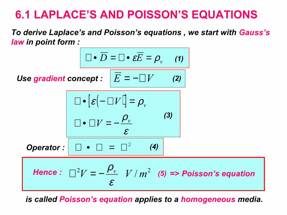
To derive Laplace’s and Poisson’s equations , we start with Gauss’s law in point form :

vED ρε =•∇=•∇

VE −∇=Use gradient concept :

( )[ ]

ερ

ρε

v

v

V

V

−=∇•∇

=∇−•∇

2∇=∇•∇Operator :

Hence :

(1)

(2)

(3)

(4)

(5) => Poisson’s equation

is called Poisson’s equation applies to a homogeneous media.

22 / mVV v

ερ−=∇

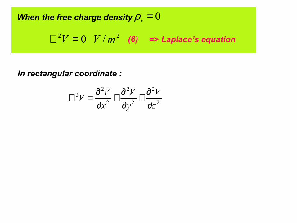
0=vρ When the free charge density

=> Laplace’s equation(6)22 / 0 mVV =∇

2

2

2

2

2

22

z

V

y

V

x

VV

∂∂+

∂∂+

∂∂=∇

In rectangular coordinate :

6.2 UNIQUENESS THEOREM

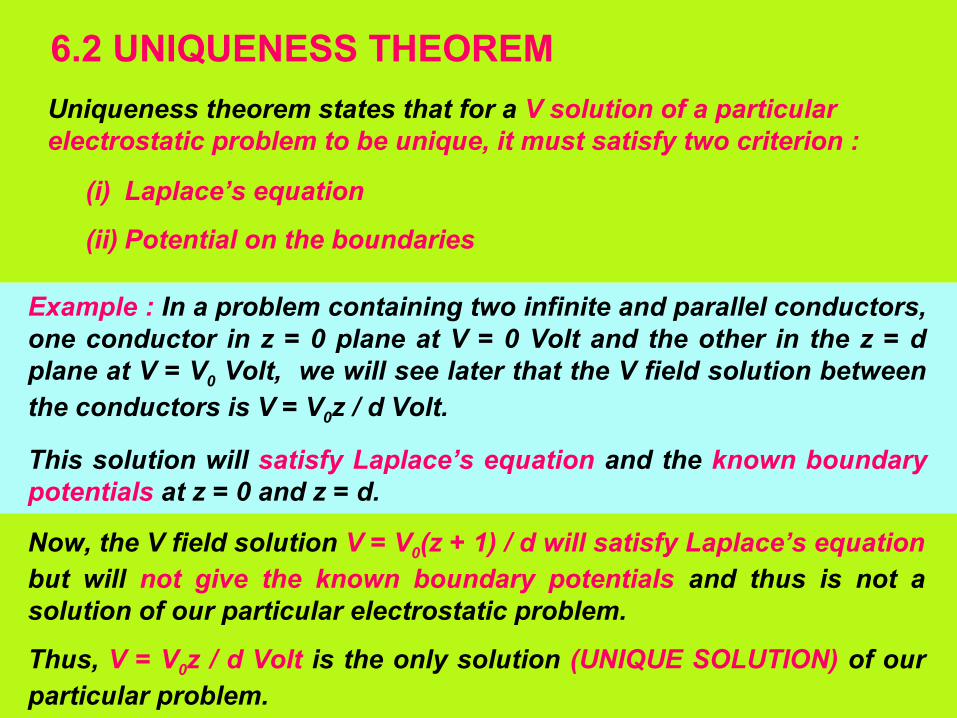
Uniqueness theorem states that for a V solution of a particular electrostatic problem to be unique, it must satisfy two criterion :

(i) Laplace’s equation

(ii) Potential on the boundaries

Example : In a problem containing two infinite and parallel conductors, one conductor in z = 0 plane at V = 0 Volt and the other in the z = d plane at V = V0 Volt, we will see later that the V field solution between the conductors is V = V0z / d Volt.

This solution will satisfy Laplace’s equation and the known boundary potentials at z = 0 and z = d.

Now, the V field solution V = V0(z + 1) / d will satisfy Laplace’s equation but will not give the known boundary potentials and thus is not a solution of our particular electrostatic problem.

Thus, V = V0z / d Volt is the only solution (UNIQUE SOLUTION) of our particular problem.

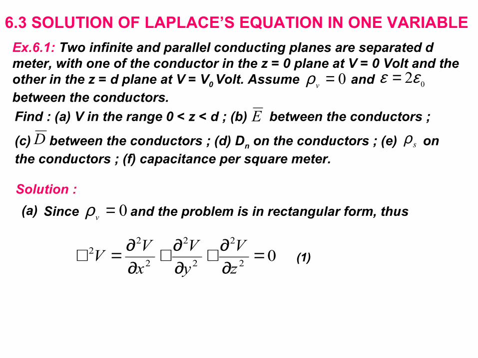
6.3 SOLUTION OF LAPLACE’S EQUATION IN ONE VARIABLE

Ex.6.1: Two infinite and parallel conducting planes are separated d meter, with one of the conductor in the z = 0 plane at V = 0 Volt and the other in the z = d plane at V = V0 Volt. Assume and between the conductors.

02εε =0=vρ

Find : (a) V in the range 0 < z < d ; (b) between the conductors ;

(c) between the conductors ; (d) Dn on the conductors ; (e) on the conductors ; (f) capacitance per square meter.

E

D sρ

Solution :

0=vρSince and the problem is in rectangular form, thus

02

2

2

2

2

22 =

∂∂+

∂∂+

∂∂=∇

z

V

y

V

x

VV (1)

(a)

0

0

2

2

2

2

22

=

=

=∂∂=∇

dz

V

dz

d

dz

Vd

z

VV

We note that V will be a function of z only V = V(z) ; thus :

BAzV

Adz

dV

+=

=Integrating twice :

where A and B are constants and must be evaluated using given potential values at the boundaries :

00

===

BVz

dVA

VAdVdz

/0

0

=→==

=

(2)

(3)

(4)

(5)

(6)

(7)

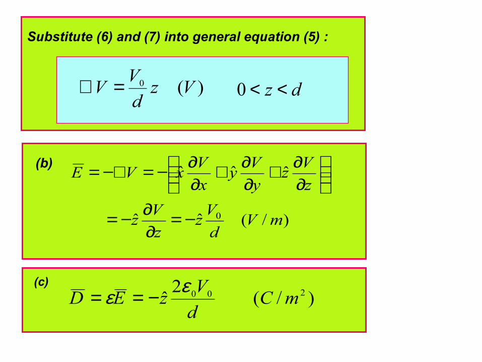
)(0 Vzd

VV =∴

Substitute (6) and (7) into general equation (5) :

dz <<0

)/(ˆˆ

ˆˆˆ

0 mVd

Vz

z

Vz

z

Vz

y

Vy

x

VxVE

−=∂∂−=

∂∂+

∂∂+

∂∂−=−∇=(b)

)/(2

ˆ 200 mCd

VzED

εε −==(c)

)/(2

)ˆ(2

ˆˆ

2

ˆ2

ˆˆ

200

00

00

000

mCd

V

zd

VznD

d

V

zd

VznD

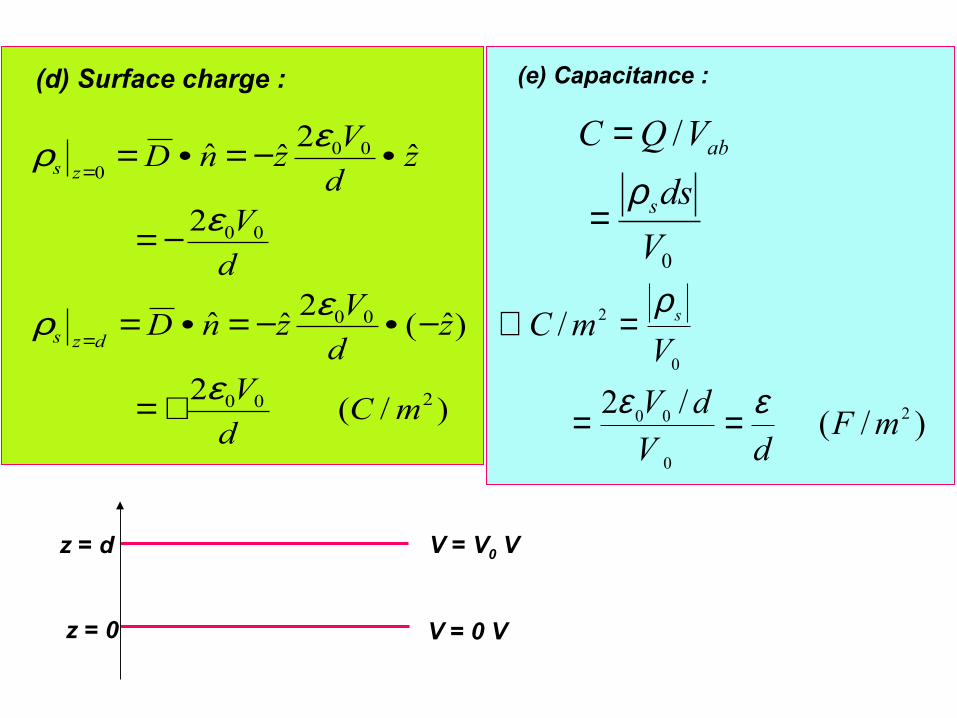
dzs

zs

ε

ερ

ε

ερ

+=

−•−=•=

−=

•−=•=

=

=

(d) Surface charge :

0

/

V

ds

VQC

s

ab

ρ=

=

)/(/2

/

2

0

00

0

2

mFdV

dV

VmC s

εε

ρ

==

=∴

(e) Capacitance :

z = 0

z = d

V = 0 V

V = V0 V

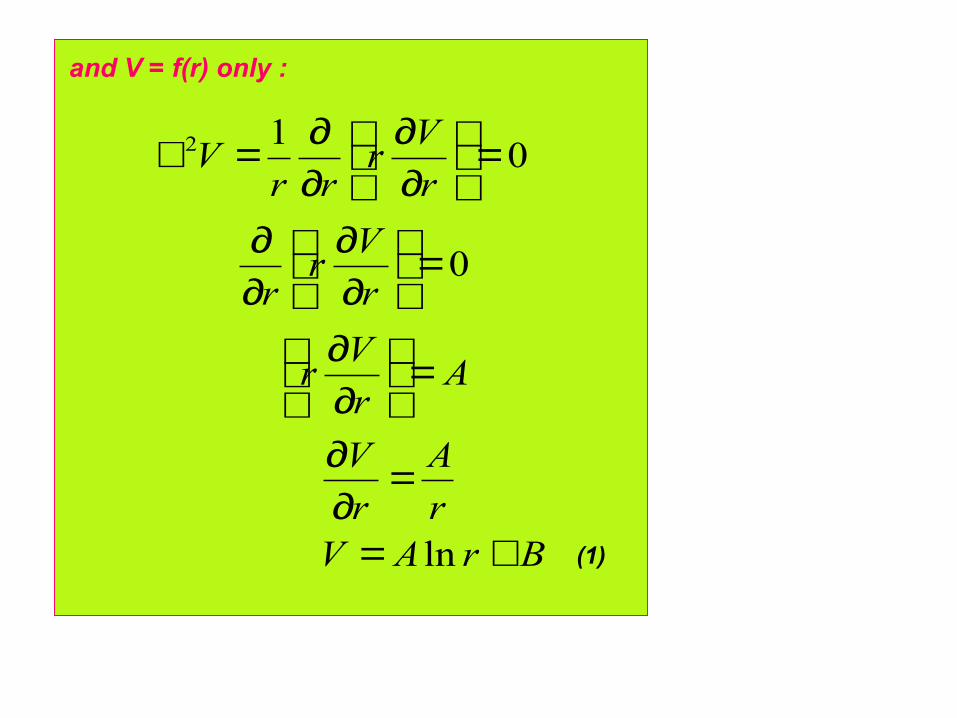
Ex.6.2: Two infinite length, concentric and conducting cylinders of radii a and b are located on the z axis. If the region between cylinders are charged free and , V = V0 (V) at a, V = 0 (V) at b and b > a. Find the capacitance per meter length.

03εε =

Solution : Use Laplace’s equation in cylindrical coordinate :

and V = f(r) only :

011

2

2

2

2

22 =

∂∂+

∂∂+

∂∂

∂∂=∇

z

VV

rr

Vr

rrV

φ

BrAVr

A

r

V

Ar

Vr

r

Vr

r

r

Vr

rrV

+=

=∂∂

=

∂∂

=

∂∂

∂∂

=

∂∂

∂∂=∇

ln

0

012

and V = f(r) only :

(1)

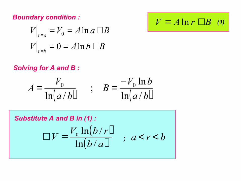
BrAV += ln

BbAV

BaAVV

br

ar

+==

+==

=

=

ln0

ln0

Boundary condition :

( ) ( )babV

Bba

VA

/ln

ln;

/ln00 −

==

Solving for A and B :

( )( )ab

rbVV

/ln

/ln0=∴

Substitute A and B in (1) :

(1)

bra <<;

( )

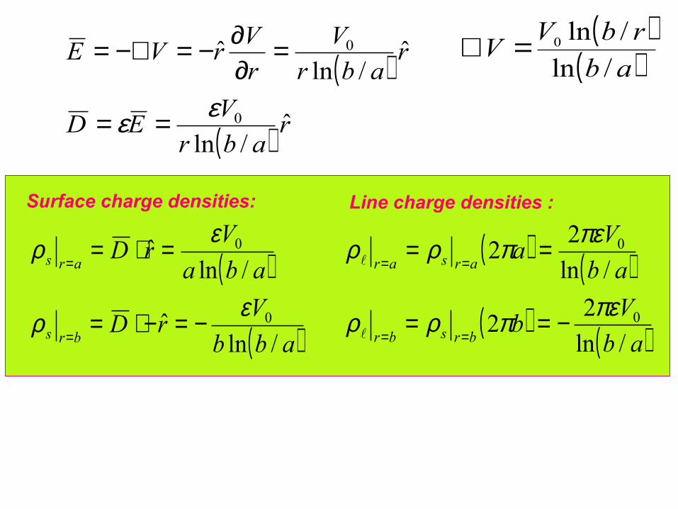
( ) rabr

VED

rabr

V

r

VrVE

ˆ/ln

ˆ/ln

ˆ

0

0

εε ==

=∂∂−=−∇=

( )( )ab

rbVV

/ln

/ln0=∴

( )

( )abb

VrD

aba

VrD

brs

ars

/lnˆ

/lnˆ

0

0

ερ

ερ

−=−⋅=

=⋅=

=

=

Surface charge densities:

( ) ( )( ) ( )ab

Vb

ab

Va

brsbr

arsar

/ln

22

/ln

22

0

0

πεπρρ

πεπρρ

−==

==

==

==

Line charge densities :

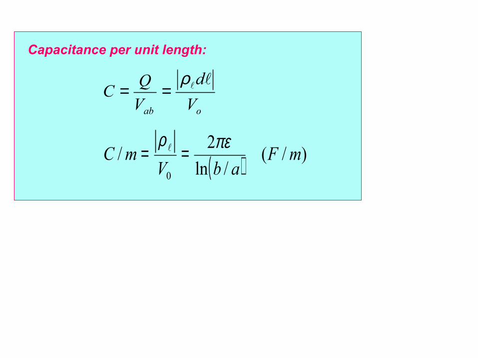
oab V

d

V

QC

ρ==

Capacitance per unit length:

( ) )/(/ln

2/

0

mFabV

mCπερ

==

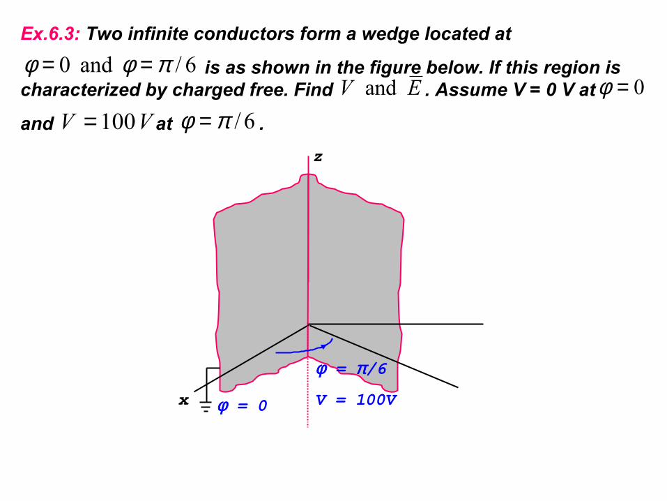
6/ and 0 πφφ ==0=φ

VV 100= 6/πφ =EV and

Ex.6.3: Two infinite conductors form a wedge located at

is as shown in the figure below. If this region is characterized by charged free. Find . Assume V = 0 V at

and at .

z

x φ = 0

φ = π/6

V = 100V

Solution : V = f ( φ ) in cylindrical coordinate :

01

2

2

2

2 ==∇φdVd

rV

BAV

Ad

dV

d

Vd

+=

=

=

φφ

φ0

2

2

π

ππφ

φ

/600

)6/(100

0

6/

0

=

==

==

=

=

A

AV

BV

Boundary condition :

Hence :

φπ

φφ

ˆ600

ˆ1

r

d

dV

rVE

−=

−=−∇=

φπ

600=V

6/0 πφ ≤≤for region :

( ) BAV

A

d

dV

Ad

dV

d

dV

d

d

d

dV

d

d

rV

+=

=

=

=

=

=∇

2/tanlnsin

sin

0sin

0sinsin

12

2

θθθ

θθ

θθ

θ

θθ

θθ

θ = π/10

θ = π/6

V = 50 V

xy

z

6/ and 10/ πθπθ ==E

Ex.6.4: Two infinite concentric conducting cone located at

10/πθ =. The potential V = 0 V at

6/πθ =and V = 50 V at . Find V and between the two conductors.

Solution : V = f ( ) in spherical coordinate :θ

( )2/tanlnsin

θθ

θ =∫d

Using :

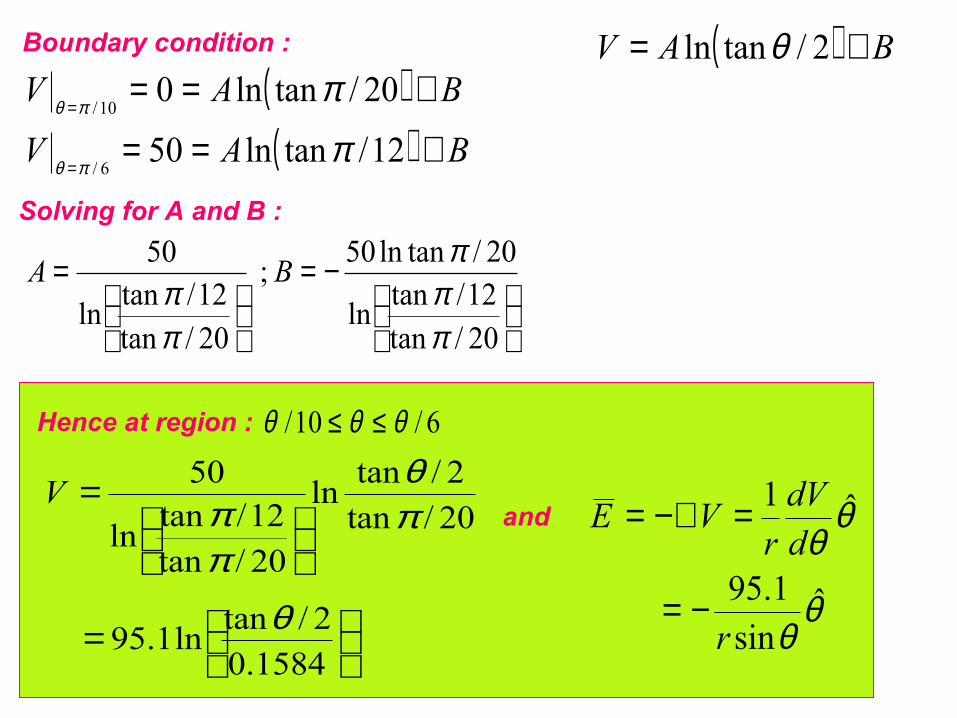
( ) BAV += 2/tanln θ( )( ) BAV

BAV

+==

+==

=

=

12/tanln50

20/tanln0

6/

10/

π

π

πθ

πθ

Boundary condition :

Solving for A and B :

−=

=

20/tan12/tan

ln

20/tanln50 ;

20/tan12/tan

ln

50

ππ

π

ππ

BA

=

=

1584.0

2/tanln1.95

20/tan

2/tanln

20/tan

12/tanln

50

θ

πθ

ππ

V

θθ

θθˆ

sin1.95

ˆ1

r

ddVr

VE

−=

=−∇=

6/10/ θθθ ≤≤Hence at region :

and

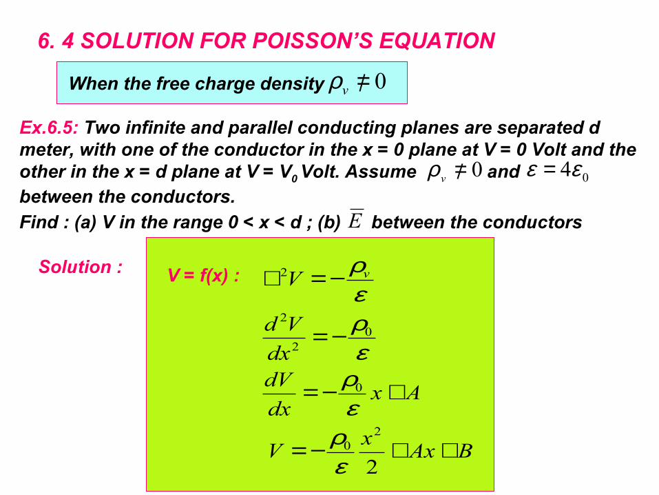
6. 4 SOLUTION FOR POISSON’S EQUATION

0=vρ When the free charge density

Ex.6.5: Two infinite and parallel conducting planes are separated d meter, with one of the conductor in the x = 0 plane at V = 0 Volt and the other in the x = d plane at V = V0 Volt. Assume and between the conductors.

04εε =0=vρ

Find : (a) V in the range 0 < x < d ; (b) between the conductors E

Solution :

BAxx

V

Axdx

dVdx

Vd

V v

++−=

+−=

−=

−=∇

2

20

0

02

2

2

ερ

ερερερV = f(x) :

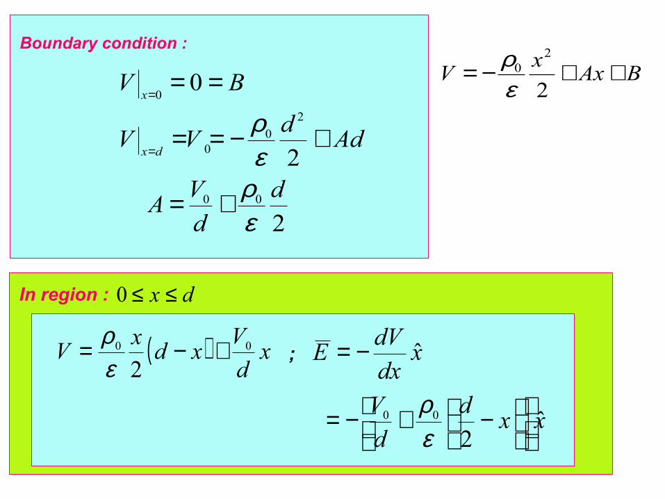
2

2

0

00

2

00

0

d

d

VA

Add

VV

BV

dx

x

ερερ

+=

+−==

==

=

=

Boundary condition :

BAxx

V ++−=2

20

ερ

dx ≤≤0In region :

( ) xd

Vxd

xV 00

2+−=

ερ

xxd

d

V

xdx

dVE

ˆ2

ˆ

00

−+−=

−=

ερ

;

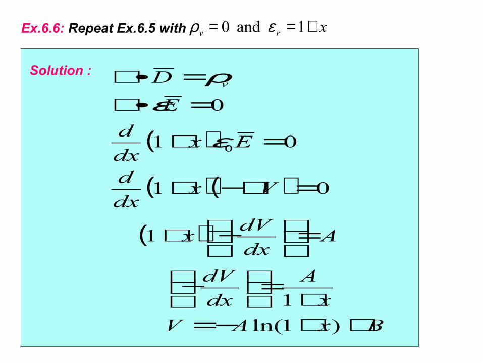
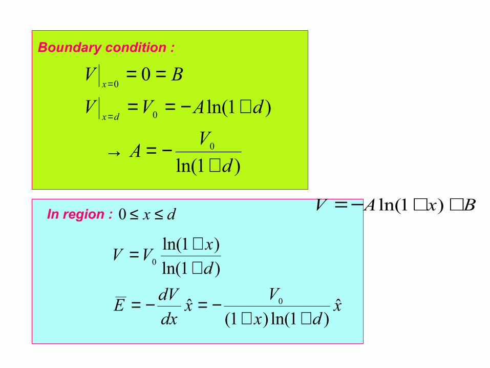
xrv +== 1 and 0 ερEx.6.6: Repeat Ex.6.5 with

( )

( )( )

( )

BxAV

x

A

dx

dV

Adx

dVx

Vxdx

d

Exdx

d

E

D v

++−=+

=

−

=

−+

=∇−+

=+

=•∇=•∇

)1ln(

1

1

01

01

0

0ε

ερSolution :

)1ln(

)1ln(

0

0

0

0

d

VA

dAVV

BV

dx

x

+−=→

+−==

==

=

=

Boundary condition :

xdx

Vx

dx

dVE

d

xVV

ˆ)1ln()1(

ˆ

)1ln(

)1ln(

0

0

++−=−=

++=

dx ≤≤0In region :BxAV ++−= )1ln(