Embed Size (px)
Citation preview

Chapter 3 Review
Profit
Price Elasticity
RPMYield
ASMUnit Cost
Time Elasticity
RPM# FlightsQOS Elasticity
RPMQOS
QOSUnit Cost
Spill
Dem
and
Operating Expense
Revenue
EconomiesOf Scale

Fundamentals of Pricing and Revenue Management
Chapter 4
Lesson 3

Outline
• Airline Pricing and O‐D Markets– Pricing Strategies
– Price Discrimination vs. Product Differentiation
• Airline Differential Pricing– “willingness to pay”(WTP)
• Airline Revenue Management

Airline Pricing and O‐D MarketsPricing Strategies

Airline Prices and O‐D Markets
• Pricing – refers to the process of determining fare levels, combined with various service amenities and restrictions, for a set of fare products in an origin‐destination market
• Revenue Management – is the subsequent process of determining how many seats to make available at each fare level
• Regulated Pricing – the Civil Aeronautics Board (CAB) used a mileage‐based formula to ensure equal prices for equal distances
• “Deregulated” or Liberalized Pricing – Different O‐D markets can have prices not related to distance traveled, or even the airline’s operating costs, as airlines match low‐fare competitors to maintain market presence and share of traffic– Its possible that low‐volume O‐D markets are more costly to serve per
passenger basis will see higher prices than high‐density O‐D markets, even if similar distances are involved

Theoretical Pricing Strategies
• For determining prices to charge in an O‐D market, airlines can utilize one of following economic principles:– Cost‐based pricing– Demand‐based pricing– Service‐based pricing
• In practice, most airline pricing strategies reflect a mix of these theoretical principles:– Prices are also highly affected by competition in each O‐D
Market– In the US, severe competition in some markets has led to
“price‐based costing”, meaning airlines must reduce costs to be able to match low‐fare competitors and passengers’ price expectations

Price Discrimination vs. Product Differentiation
• Price discrimination:– The practice of charging different prices for same product with same costs of production
– Based solely on different consumers’ “willingness to pay”
• Product differentiation:– Charging different prices for products with different characteristics and costs of production
• Current airline fare structures reflect both strategies:– Differential Pricing based on differentiated fare products– But higher prices for fare products targeted at business travelers are clearly based on their willingness to pay
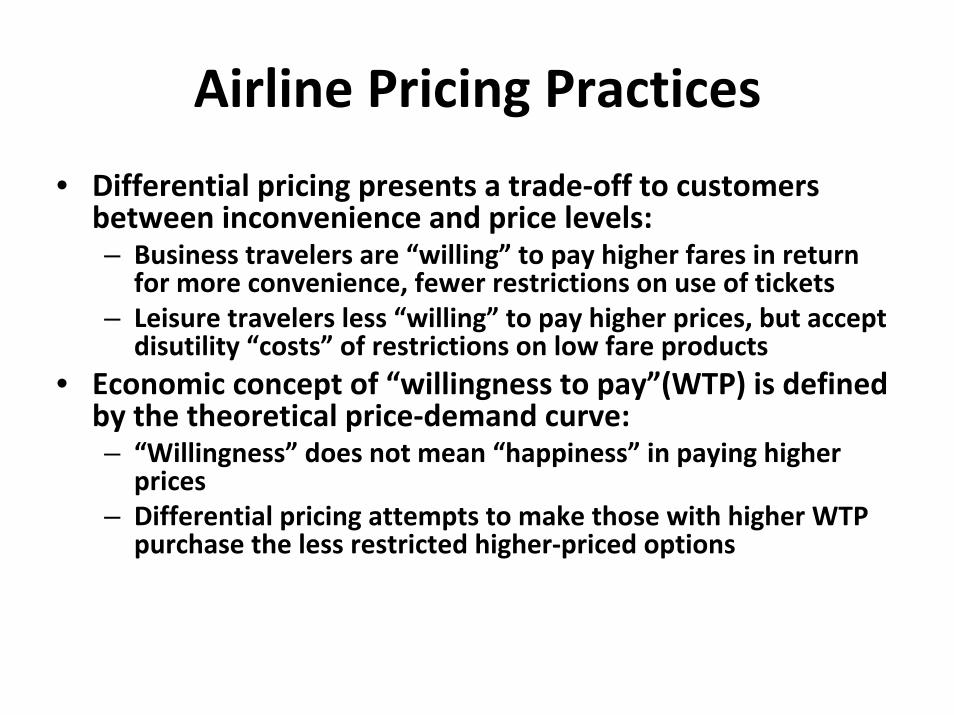
Airline Pricing Practices
• Differential pricing presents a trade‐off to customers between inconvenience and price levels:– Business travelers are “willing” to pay higher fares in return
for more convenience, fewer restrictions on use of tickets– Leisure travelers less “willing” to pay higher prices, but accept
disutility “costs” of restrictions on low fare products• Economic concept of “willingness to pay”(WTP) is defined
by the theoretical price‐demand curve:– “Willingness” does not mean “happiness” in paying higher
prices– Differential pricing attempts to make those with higher WTP
purchase the less restricted higher‐priced options

Differential Pricing Theory (circa 2000)
• Market segments with different “willingness to pay” for air travel
• Different “fare products”offered to business versus leisure travelers
• Prevent diversion by setting restrictions on lower fare products and limiting seats available
• Increased revenues and higher load factors than any single fare strategyDemand
Price

Airline Differential Pricing

Why Differential Pricing?• It allows the airline to increase total flight revenues with little impact
on total operating costs:
– Incremental revenue generated by discount fare passengers who otherwise would not fly
– Incremental revenue from high fare passengers willing to pay more
– Studies have shown that most “traditional” high‐cost airlines could not cover total operating costs by offering a single fare level
• Consumers can also benefit from differential pricing:
– Most notably, discount passengers who otherwise would not fly
– It is also conceivable that high fare passengers pay less and/orenjoy more frequency given the presence of low fare passengers
• If airline could charge a different price for each customer based on their WTP, its revenues would be close to the theoretical maximum

Market Segmentation
• Business and Leisure travelers are the two traditional segments targeted by the airlines in their different pricing efforts– First Class, Business Class, and Economy– Restrictions on advance purchase, use, and refundability
• A wide enough range of fare product options at different price levels should be offered to capture as much revenue potential from the market price‐demand curve as possible

Traditional Approach: Restrictions on Lower Fares
• Progressively more severe restrictions on low fare products designed to prevent diversion:– Lowest fares have advance purchase and minimum stay requirements , as well as cancellation and change fees
– Restrictions increase the inconvenience or “disutility cost” of low fares to travelers with high WTP, forcing them to pay more
– Studies show “Saturday night minimum stay” condition to be most effective in keeping business travelers from purchasing low fares
• Still, it is impossible to achieve perfect segmentation:– Some travelers with high WTP can meet restrictions– Many business travelers often purchase restricted fares

Example: Restriction Disutility Costs

Example: BOS‐SEA Traditional Fares
Round‐Trip Fare ($)
Cls Advance Purchase
Minimum Stay
Change Fee?
Comment
$458 N 21 days Sat. Night Yes Tue/Wed/Sat
$707 M 21 days Sat. Night Yes Tue/Wed
$760 M 21 days Sat. Night Yes Thur‐Mon
$927 H 14 days Sat. Night Yes Tue/Wed
$1001 H 14 days Sat. Night Yes Thur‐Mon
$2083 B 3 days None No 2xOW Fare
$2262 Y None None No 2xOW Fare
$2783 F None None No First Class
Figure 4.5

Fare Simplification:Less Restricted and Lower Fares
• Recent trend toward “simplified” fares –compressed fare structures with fewer restrictions– Initiated by some LFAs and America West, followed by Alaska – Most recently, implemented in all US domestic markets by
Delta, matched selectively by legacy competitors• Simplified fare structures characterized by:
– No Saturday night stay restrictions, but advance purchase and non‐refundable/change fees
– Revenue management systems still control number of seats sold at each fare level
• Higher load factors, but 10‐15% lower revenues:– Significantly higher diversion with fewer restrictions

Example: BOS‐ATL Simplified FaresDelta Air Lines, April 2005

Revenue Impact of Each “Simplification”

Impacts on Differential Pricing Model
• Drop in business demand and willingness to pay highest fares
• Greater willingness to accept restrictions on lower fares
• Reduction in lowest fares to stimulate traffic and respond to LCCs
• Result is lower total revenue and unit RASM despite stable load factorsDemand
Price

Airline Revenue Management

Airline Revenue Management
• Two components of airline revenue maximization:Differential Pricing:– Various “fare products” offered at different prices for travel in the same O‐D market
Yield Management (YM):– Determines the number of seats to be made available to each “fare class” on a flight, by setting booking limits on low fare seats
• Typically, YM takes a set of differentiated prices/products and flight capacity as given:– With high proportion of fixed operating costs for a committed flight schedule, revenue maximization to maximize profits

Why Call it “Yield Management”?
• Main objective of YM is to protect seats for later‐booking, high‐fare business passengers.
• YM involves tactical control of airline’s seat inventory:– But too much emphasis on yield (revenue per RPM) can lead
to overly severe limits on low fares, and lower overall load factors
– Too many seats sold at lower fares will increase load factors but reduce yield, adversely affective total revenues
• Revenue maximization is proper goal: – Requires proper balance of load factor and yield
• Many airlines now refer to “Revenue Management”(RM) instead of “Yield Management”

Seat Inventory Control Approaches
Figure 4.11

Computerized RM Systems
• Size and complexity of a typical airline’s seat inventory control problem requires a computerized RM system
• Consider a US Major airline with:500 flight legs per day15 booking classes330 days of bookings before departure
• At any point in time, this airline’s seat inventory consists of almost 2.5 million booking limits:– This inventory represents the airline’s potential for profitable
operation, depending on the revenues obtained– Far too large a problem for human analysts to monitor alone

Typical 3rd Generation RM System
• Collects and maintains historical booking data by flight and fare class, for each past departure date.
• Forecasts future booking demand and no‐show rates by flight departure date and fare class.
• Calculates limits to maximize total flight revenues:– Overbooking levels to minimize costs of spoilage/denied boardings
– Booking class limits on low‐value classes to protect high‐fare seats
• Interactive decision support for RM analysts:– Can review, accept or reject recommendations
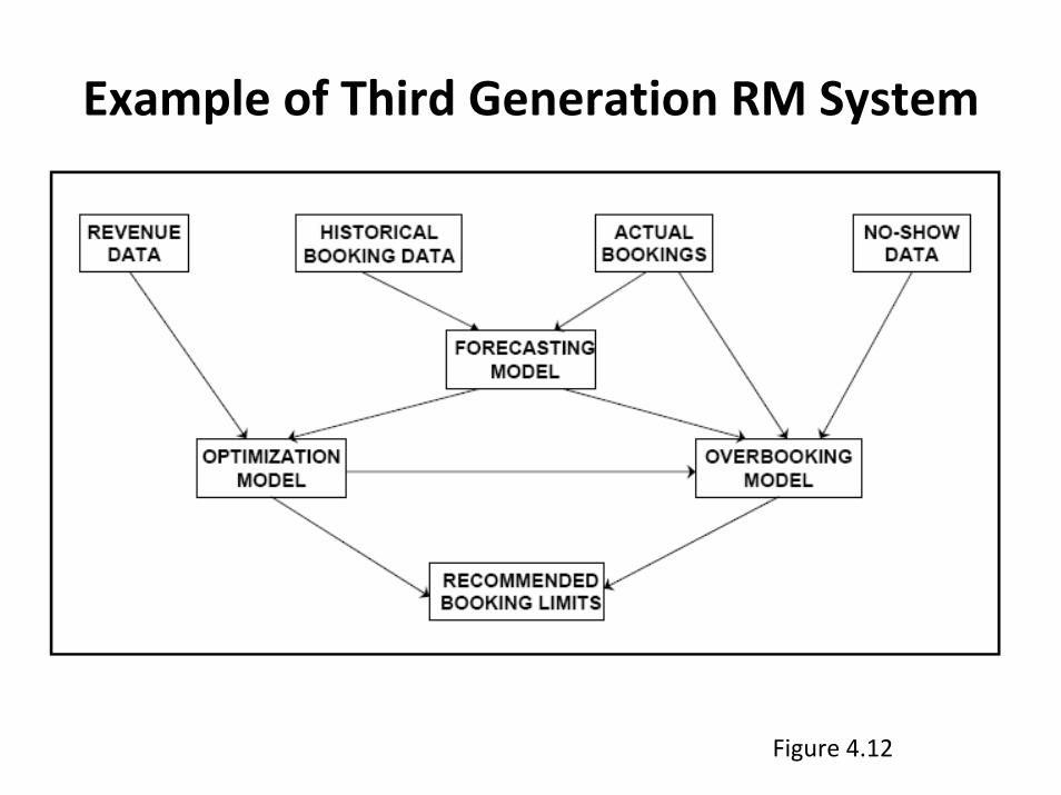
Example of Third Generation RM System
Figure 4.12

Revenue Management Techniques
• Overbooking– Accept reservations in excess of aircraft capacity to overcome loss of revenues due to passenger “no‐show”effects
• Fare Class Mix (Flight Leg Optimization)– Determine revenue‐maximizing mix of seats available to each booking (fare) class on each flight departure
• Traffic Flow (O‐D) Control (Network Optimization)– Further distinguish between seats available to short‐haul (one‐leg) vs. long‐haul (connecting) passengers, to maximize total network revenues

Flight Overbooking
• Determine maximum number of bookings to accept for a given physical capacity.
• Minimize total costs of denied boardings and spoilage(lost revenue).
• U.S. domestic no‐show rates can reach 15‐20 percent of final pre‐departure bookings:– On peak holiday days, when high no‐shows are least desirable
– Average no‐show rates have dropped, to 10‐15% with more fare penalties and better efforts by airlines to firm up bookings
• Effective overbooking can generate as much revenue gain as fare class seat allocation.
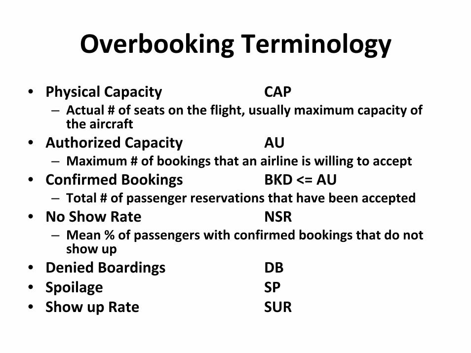
Overbooking Terminology
• Physical Capacity CAP– Actual # of seats on the flight, usually maximum capacity of
the aircraft • Authorized Capacity AU
– Maximum # of bookings that an airline is willing to accept• Confirmed Bookings BKD <= AU
– Total # of passenger reservations that have been accepted• No Show Rate NSR
– Mean % of passengers with confirmed bookings that do not show up
• Denied Boardings DB• Spoilage SP• Show up Rate SUR

Overbooking Models
• Overbooking models try to minimize:– Total costs of overbooking (denied boardings plus spoilage)
– Risk of “excessive” denied boardings on individual flights, for customer service reasons
• Mathematical overbooking problem:– Find OV > 1.00 such that AU = CAP * OV
– But actual no‐show rate is highly uncertain

Manual/Judgmental Approach
• Relies on judgment of human analyst to set overbooking level:– Based on market experience and perhaps recent no‐show history
– Tendency to choose OV = 1+NSR (or lower)
– Tendency to focus on avoidance of DB
• For CAP=100 and mean NSR=.20, then:AU = 100 (1.20) = 120

Deterministic Model
• Based on estimate of mean NSR from recent history:– Assume that BKD=AU (“worst case”scenario)
– Find AU such thatAU ‐NSR*AU = CAP
– Or, AU = CAP/(1‐NSR)
• For CAP=100 and NSR=0.20, then:AU = 100/(1‐.20) = 125

Probabilistic/Risk Model
• Incorporates uncertainty about NSR for future flight:– Standard deviation of NSR from history, STD
• Find AU that will keep DB=0, assuming BKD=AU, with a 95% level of confidence:– Assume a probability (Gaussian) distribution of no‐show rates
• Keep show‐ups less than or equal to CAP, when BKD=AU:– Find SUR*, so that AU x SUR* = CAP,
and Prob[AU x SUR* > CAP] = 5%• From Gaussian distribution, SUR* will satisfy:
Z = 1.645 = SUR* ‐SURSTD
where SUR = mean show‐up rateSTD = standard deviation of show‐up rate

Probabilistic/Risk Model (cont.)
• Optimal AU given CAP, SUR, STD with objective of DB=0 with 95% confidence is:AU = CAP = CAP
SUR + 1.645 STD 1‐NSR + 1.645 STD
• In our example, with STD= 0.05 & NSR=.20:AU = 100 / (1‐0.20 + 1.645*0.05) = 113
• The larger STD, the larger the denominator and the lower the optimal AU, due to increased risk/uncertainty about no‐shows.

More Overbooking Terminology
• Waitlisted passengers WL
• Go‐show passengers GS
• Stand‐by passengers SB
• No‐shows NS
• Show‐ups SU
• Passengers Boarded PAX
• Voluntary DB VOLDB

Probabilistic Model Extensions
• Reduce level of confidence of exceeding DB limit:– Z factor in denominator will decrease, causing increase in AU
• Increase DB tolerance to account for voluntary DB:– Numerator becomes (CAP+ VOLDB), increases AU
• Include forecasted empty F or C cabin seats for upgrading:– Numerator becomes (CAP+FEMPTY+CEMPTY), increases AU– Empty F+C could also be “overbooked”
• Deduct group bookings and overbook remaining capacity only:– Firm groups much more likely to show up– Flights with firm groups should have lower AU
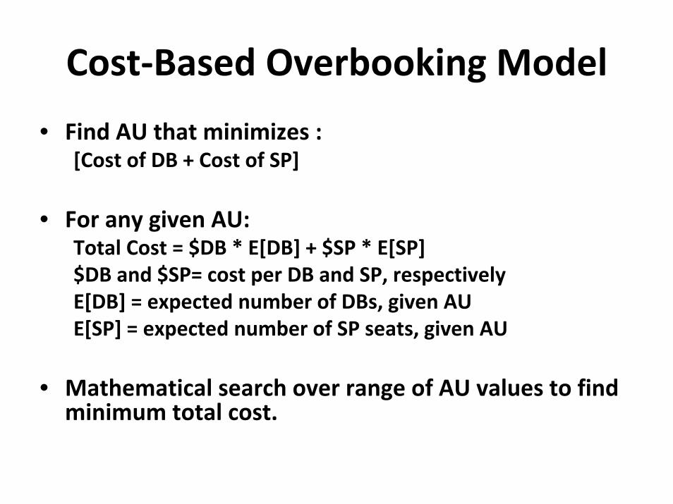
Cost‐Based Overbooking Model
• Find AU that minimizes :[Cost of DB + Cost of SP]
• For any given AU:Total Cost = $DB * E[DB] + $SP * E[SP]$DB and $SP= cost per DB and SP, respectivelyE[DB] = expected number of DBs, given AUE[SP] = expected number of SP seats, given AU
• Mathematical search over range of AU values to find minimum total cost.

Example: Cost‐Based Overbooking Model

Cost Inputs to Overbooking Model
• Denied Boarding Costs:– Cash compensation for involuntary DB
– Free travel vouchers for voluntary DB
– Meal and hotel costs for displaced passengers
– Space on other airlines
– Cost of lost passenger goodwill costs
• Many airlines have difficulty providing accurate DB cost inputs to these models.

Dynamic Revision and Intervention
• RM systems revise forecasts and re‐optimize booking limits at numerous “checkpoints” of the booking process:– Monitor actual bookings vs. previously forecasted demand – Re‐forecast demand and re‐optimize at fixed checkpoints or
when unexpected booking activity occurs– Can mean substantial changes in fare class availability from
one day to the next, even for the same flight departure• Substantial proportion of fare mix revenue gain comes
from dynamic revision of booking limits:– Human intervention is important in unusual circumstances,
such as “unexplained” surges in demand due to special events

Current State of RM Practice
• Most of the top 25 world airlines (in terms of revenue) have implemented 3rd generation RM systems.
• Many smaller carriers are still trying to make effective use of leg/fare class RM– Lack of company‐wide understanding of RM principles– Historical emphasis on load factor or yield, not revenue– Excessive influence and/or RM abuse by dominant sales and
marketing departments– Issues of regulation, organization and culture
• About a dozen leading airlines are looking toward network O‐D control development and implementation– These carriers could achieve a 2‐5 year competitive advantage
with advanced revenue management systems

Single‐Leg Seat Allocation Problem
• Given for a future flight leg departure:– Total booking capacity of (typically) the coach compartment
– Several fare (booking) classes that share the same inventory of seats in the compartment
– Forecasts of future booking demand by fare class
– Revenue estimates for each fare (booking) class
• Objective is to maximize total expected revenue:– Allocate seats to each fare class based on value

Cost Inputs (cont’d)
• Spoilage Costs:– Loss of revenue from seat that departed empty
• What is best measure of this lost revenue:– Average revenue per seat for leg?– Highest fare class revenue on leg (since closed flights lose late‐booking passengers)?
– Lowest fare class revenue on leg (since increased AU would have allowed another discount seat)?
• Specifying spoilage costs is just as difficult.

Voluntary vs. Involuntary DBs
• Comprehensive Voluntary DB Program:– Requires training and cooperation of station crews
– Identify potential volunteers at check‐in
– Offer as much “soft” compensation as needed to make the passenger happy
• US airlines very successful in managing DBs:– 2007 involuntary DB rate was 1.12 per 10,000
– Over 90% of DBs in U.S. are volunteers
– Good treatment of volunteers generates goodwill

Flight Leg Revenue Optimization
• Given for a future flight leg departure:– Total booking capacity of (typically) the coach compartment
– Several fare (booking) classes that share the same inventory of seats in the compartment
– Forecasts of future booking demand by fare class
– Revenue estimates for each fare (booking) class
• Objective is to maximize total expected revenue:– Allocate seats to each fare class based on value
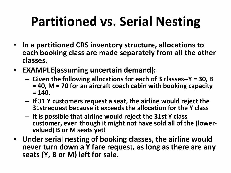
Partitioned vs. Serial Nesting
• In a partitioned CRS inventory structure, allocations to each booking class are made separately from all the other classes.
• EXAMPLE(assuming uncertain demand):– Given the following allocations for each of 3 classes‐‐Y = 30, B
= 40, M = 70 for an aircraft coach cabin with booking capacity = 140.
– If 31 Y customers request a seat, the airline would reject the 31strequest because it exceeds the allocation for the Y class
– It is possible that airline would reject the 31st Y class customer, even though it might not have sold all of the (lower‐valued) B or M seats yet!
• Under serial nesting of booking classes, the airline would never turn down a Y fare request, as long as there are any seats (Y, B or M) left for sale.

Serially Nested Buckets

Deterministic Seat Allocation/Protection
• If we assume that demand is deterministic (or known with certainty), it would be simple to determine the fare class seat allocations– Start with highest fare class and allocate/protect exactly the
number of seats predicted for that class, and continue with the next lower fare class until capacity is reached.
• EXAMPLE: 3 fare classes (Y, B, M)– Demand for Y = 30, B = 40, M = 85– Capacity = 140
• Deterministic decision: Protect 30 for Y, 40 for B, and allocated 70 for M (i.e., spill 15 M requests)
• Nested booking limits Y=140 B=110 M=70

EMSRb Model for Seat Protection:Assumptions
• Basic modeling assumptions for serially nested classes:– demand for each class is separate and independent of demand in other classes.
– demand for each class is stochastic and can be represented bya probability distribution
– lowest class books first, in its entirety, followed by the next lowest class, etc.
– booking limits are only determined once (i.e., static optimization model)

EMSRb Model Calculations
• Because higher classes have access to unused lower class seats, the problem is to find seat protection levels for higher classes, and booking limits on lower classes
• To calculate the optimal protection levels:Define Pi(Si) = probability that Xi>Si,
where Siis the number of seats made available to class i, Xiis the random demand for class i
EMSRb Calculations (cont’d)
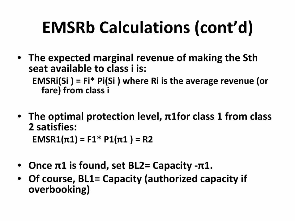
• The expected marginal revenue of making the Sth seat available to class i is:EMSRi(Si ) = Fi* Pi(Si ) where Ri is the average revenue (or fare) from class i
• The optimal protection level, π1for class 1 from class 2 satisfies:EMSR1(π1) = F1* P1(π1 ) = R2
• Once π1 is found, set BL2= Capacity ‐π1.• Of course, BL1= Capacity (authorized capacity if overbooking)

Example Calculation
• Consider the following flight leg example:Class Mean Fcst. Std. Dev. FareY 10 3 1000B 15 5 700M 20 7 500Q 30 10 350
• •To find the protection for the Y fare class, we want to find the largest value of πY for which EMSRY(πY ) = FY* PY(πY ) >RB

Example (cont’d)
EMSRY(πY ) = 1000 * PY(πY ) >700 PY(πY ) >0.70
where PY (πY ) = probability that XY>πY.
• If we assume demand in Y class is normally distributed with mean, standard deviation given earlier, then we can create a standardized normal random variable as (XY ‐10)/3.

Probability Calculations• Next, we use Excel or go to the Standard Normal Cumulative Probability Table for different “guesses” for πY. For example,
for πY = 7, Prob { (XY ‐10)/3 >(‐10)/3 } = 0.8417 for πY = 8, Prob { (XY ‐10)/3 >(‐10)/3 } = 0.7478 for πY = 9, Prob { (XY ‐10)/3 >(‐10)/3 } = 0.639
• So, we can see that πY = 8 is the largest integer value of πY that gives a probability >0.7 and therefore we will protect 8 seats for Y class!

Network Revenue Management:Origin‐Destination Control
• Vast majority of world airlines still practice “fare class control”:– High‐yield (“full”) fare types in top booking classes
– Lower yield (“discount”) fares in lower classes
– Designed to maximize yields, not total revenues
• Seats for connecting itineraries must be available in same class across all flight legs:– Airline cannot distinguish among itineraries
– “Bottleneck”legs can block long haul passengers

Yield‐Based Fare Class Structure (Example)

Connecting Flight Network Example
FRA
JFK HKG
NCE
LH100
LH200LH300

The O‐D Control Mechanism
• Revenue maximization over a network of connecting flights requires two strategies:1. Increase availability to high‐revenue, long‐haul
passengers, regardless of yield;2. Prevent long‐haul passengers from displacing
high‐yield short‐haul passengers on full flights.
• Revenue benefits of (1) outweigh risks of (2):– Probability of both connecting flights being
fully booked is low, relative to other possible outcomes
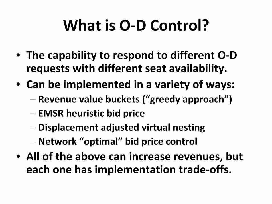
What is O‐D Control?
• The capability to respond to different O‐D requests with different seat availability.
• Can be implemented in a variety of ways:– Revenue value buckets (“greedy approach”) – EMSR heuristic bid price– Displacement adjusted virtual nesting– Network “optimal” bid price control
• All of the above can increase revenues, but each one has implementation trade‐offs.

Revenue Value Bucket Concept
• Fixed relationship between fare type and booking class is abandoned:– Booking classes (“buckets”) defined according to revenue value, regardless of fare restrictions
– Each itinerary/fare type (i.e.., “ODF”) assigned to a revenue value bucket on each flight leg
– ODF seat availability depends on value buckets
• Value concept can be implemented within existing classes or through “virtual” classes

Value Bucket Implementation
• Within Existing Booking Classes:– Fare codes need to be re‐published according to revenue value; no changes to inventory structure
– Does not require seamless CRS links, but can be confusing to travel agents and consumers
• Development of Virtual Inventory Classes:– Substantial cost of new inventory structure and mapping functions to virtual classes
– CRS seamless availability links are essential

Virtual Class Mapping by ODF Revenue Value
Figure 4.17

Value Bucket O‐D Control
• Allows O‐D control with existing RM system:– Data collection and storage by leg/value bucket– Forecasting and optimization by leg/value bucket– Different ODF requests get different availability
• But also has limitations:– Re‐bucketing of ODFs disturbs data and forecasts– Leg‐based optimization, not a network solution– Can give too much preference to long‐haul passengers (i.e..., “greedy” approach)

Displacement Cost Concept
• Actual value of an ODF to network revenue on a leg is less than or equal to its total fare:– Connecting passengers can displace revenue on down‐line (or up‐line) legs
• How to determine network value of each ODF for O‐D control purposes?– Network optimization techniques to calculate displacement cost on each flight leg
– Leg‐based EMSR estimates of displacement

Value Buckets with Displacement
• Given estimated down‐line displacement, ODFs are mapped based on networkvalue:– Network value on Leg 1 = Total fare minus sum of own‐line leg displacement costs
– Under high demand, availability for connecting passengers is reduced, locals get more seats
• Revision of displacement costs is an issue:– Frequent revisions capture demand changes, but ODF re‐mapping can disrupt bucket forecasts

Alternative Mechanism: Bid Price
• Under value bucket control, accept ODF if its network value falls into an available bucket:Network Value > Value of Last Seat on Leg; orFare ‐Displacement > Value of Last Seat
• Same decision rule can be expressed as:
• Fare > Value of Last Seat + Displacement, or• Fare > Minimum Acceptable “Bid Price”for ODF
• •Bid Prices and Value Buckets are simply two different O‐D control mechanisms.

O‐D Bid Price Control
• Much simpler inventory control mechanism than virtual buckets:
• –Simply need to store bid price value for each leg
• –Evaluate ODF fare vs. itinerary bid price at time of availability request
• –Must revise bid prices frequently to prevent too many bookings of ODFs at current bid price
• •Bid prices can be calculated with network optimization tools or leg‐based heuristics

Example: Bid Price Control
A‐‐‐‐‐‐‐B‐‐‐‐‐‐‐C‐‐‐‐‐‐‐D
• Given leg bid prices
A‐B:$35 B‐C:$240 C‐D:$160
• Availability for O‐D requests B‐C:
Bid Price = $240 Available?Y $440 YesM $315 YesB $223 NoQ $177 No

• A‐B:$35 B‐C:$240 C‐D:$160A‐C Bid Price =$275 Available?Y $519 YesM $374 YesB $292 YesQ $201 NoA‐D Bid Price = $435 Available?Y $582 YesM $399 NoB $322 NoQ $249 No

Network vs. Heuristic Models
• Estimates of displacement costs and bid prices can be derived using either approach:– Most O‐D RM software vendors claim “network optimal” solutions possible with their product
– Most airlines lack detailed data and face practical constraints in using network optimization models
– Still substantial debate among researchers about which network O‐D solution is “most optimal”
• Revenue gain, not optimality, is critical issue