Chap 2 Hyperbolic

8/2/2019 Chap 2 Hyperbolic

http://slidepdf.com/reader/full/chap-2-hyperbolic 1/14

Chapter 2

Hyperbolic equations

As we have seen, and will further argue below, the hydrodynamics equations are nothing more

than signal-propagation equations. Equations of this kind are called hyperbolic equations. The

equations of hydrodynamics are only a member of the more general class of hyperbolic equa-

tions, and there are many more examples of hyperbolic equations than just the equations of

hydrodynamics. But of course we shall focus mostly on the application to hydrodynamics. In

this chapter we shall study the mathematical properties of hyperbolic equations, and analytic

methods how to solve them for simple linear problems. This background knowledge is not only

important for understanding the nature of hydrodynamic flows, it also lies at the basis of numer-

ical hydrodynamics algorithms. Hence we go into quite some detail here.

2.1 The simplest form of a hyperbolic equation: advection

Consider the following equation:

∂ tq + u∂ xq = 0 (2.1)

where q = q(x, t) is a function of one spatial dimension and time, and u is a velocity that

is constant in space and time. This is called an advection equation, as it describes the time-

dependent shifting of the function q(x) along x with a velocity u (Fig. 2.1-left). The solution at

any time t > t0 can be described as a function of the state at time t0:

q(x, t) = q(x− ut, 0) (2.2)

This is a so-called initial value problem in which the state at any time t > t0 can be uniquely

found when the state at time t = t0 is fully given. The characteristics of this problem are straight

lines:

xchar(t) = x(0)char + ut (2.3)

This is a family of lines in the (x, t) plane, each of which is labeled by its own unique value of

x(0)char.

In this example the initial value problem is quite trivial, yet, as we will see below, this prob-

lem stands at the basis of numerical methods of hydrodynamics and is numerically surprisingly

challenging to solve!

23



24

q(x)

space

u(x)

space

q(x)

u(x)

space

conserved quantity

pure advection

space

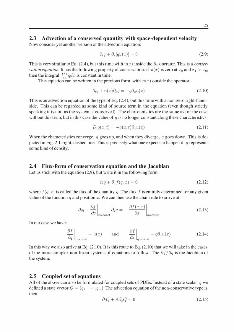
Figure 2.1. Advection of a function q(x, t) with constant velocity u (left) and space-varying

velocity u(x) (right). The space-varying velocity problem comes in two versions: the conserved

form (dashed) and the non-conserved simple advection form (dotted).

2.2 Advection with space-dependent velocityConsider now that u is a function of space: u = u(x). We get:

∂ tq + u(x)∂ xq = 0 (2.4)

This is still an advection problem, but the velocity is not constant, and therefore the solution is

somewhat more complex. Define the following variable:

ξ =

xx0

dx′

u(x′)(2.5)

for some arbitary x0. Now the solution is given as:

q(x, t) = q(x(ξ), t) = q(x(ξ − t), 0) (2.6)

where x(ξ) is the value of x belonging to the value of ξ. We see that in regions of low u(x)the function will be squeezed in x-direction while in regions of high u(x) the function will

be stretched. Fig. 2.1-right, dotted line, shows the squeezing effect for non-constant advectionvelocity.

The characteristics are:

xchar(t) = x(ξ(0)char + t) (2.7)

In this case the labeling is done with ξ(0)char and, by definition, the curves follow the flow in the

(x, t) plane.

If we define the comoving derivative Dt as Dt = ∂ t + u(x)∂ x, Eq.(2.4) translates into:

Dtq(x, t) = 0 (2.8)

This simply tells that along each flow line (characteristic) the function q remains constant, i.e. the

comoving derivative is zero.



25

2.3 Advection of a conserved quantity with space-dependent velocityNow consider yet another version of the advection equation:

∂ tq + ∂ x[qu(x)] = 0 (2.9)

This is very similar to Eq. (2.4), but this time with u(x) inside the ∂ x operator. This is a conser-

vation equation. It has the following property of conservation: if u(x) is zero at x0 and x1 > x0,

then the integral x1x0

qdx is constant in time.

This equation can be written in the previous form, with u(x) outside the operator:

∂ tq + u(x)∂ xq = −q∂ xu(x) (2.10)

This is an advection equation of the type of Eq. (2.4), but this time with a non-zero right-hand-

side. This can be regarded as some kind of source term in the equation (even though strictly

speaking it is not, as the system is conserved). The characteristics are the same as for the case

without this term, but in this case the value of q is no longer constant along these characteristics:

Dtq(x, t) = −q(x, t)∂ xu(x) (2.11)

When the characteristics converge, q goes up, and when they diverge, q goes down. This is de-

picted in Fig. 2.1-right, dashed line. This is precisely what one expects to happen if q represents

some kind of density.

2.4 Flux-form of conservation equation and the Jacobian

Let us stick with the equation (2.9), but write it in the following form:

∂ tq + ∂ xf (q, x) = 0 (2.12)

where f (q, x) is called the flux of the quantity q. The flux f is entirely determined for any given

value of the function q and position x. We can then use the chain rule to arrive at

∂ tq +∂f

∂q

x=const

∂ xq = − ∂f (q, x)

∂x

q=const

(2.13)

In our case we have:

∂f ∂qx=const

= u(x) and ∂f ∂x

q=const

= q∂ xu(x) (2.14)

In this way we also arrive at Eq. (2.10). It is this route to Eq. (2.10) that we will take in the cases

of the more complex non-linear systems of equations to follow. The ∂f/∂q is the Jacobian of

the system.

2.5 Coupled set of equationsAll of the above can also be formulated for coupled sets of PDEs. Instead of a state scalar q we

defined a state vector Q = (q1,· · ·

, qm). The advection equation of the non-conservative type is

then

∂ tQ + A∂ xQ = 0 (2.15)



26

where A is an m× m matrix. The advection equation of conservative type is

∂ tQ + ∂ x(AQ) = 0 (2.16)

The more general conservation equation is:

∂ tQ + ∂ xF = 0 (2.17)

where F = F (Q, x) is the flux. Like in the scalar case we have

∂ tQ +∂F

∂Q

x=const

∂ xQ = − ∂F (q, x)

∂x

Q=const

(2.18)

where the J ≡ ∂F/∂Q is the Jacobian of the system, which is an m × m matrix. If F is a

linear function of Q, then one can write F = AQ where A is then the Jacobian, and we arrive atEq. (2.16). If A is then also independent of x, then we arrive at Eq. (2.16).

2.6 The wave equation in vector notation: eigenvalues and eigenvectorsIn Section 1.7.1 we derived the wave equation for perturbations in an otherwise steady constant-

density constant-velocity background medium. Let us now define:

Q ≡

q1q2

=

ρ1

ρ0u1

(2.19)

We can then write Eqs. (1.56,1.57) as:

∂ t

q1q2

+

u0 1C 2s u0

∂ x

q1q2

= 0 (2.20)

We can also write this in flux conservative form:

∂ t

q1q2

+ ∂ x

f 1f 2

= 0 (2.21)

with the flux F = (f 1, f 2) given as:

F ≡

f 1f 2

=

u0 1C 2s u0

q1q2

=

u0q1 + q2

C 2s q1 + u0q2

(2.22)

or in other words, the Jacobian matrix is:

J ik =∂f i∂qk

=

u0 1C 2s u0

(2.23)

One of the advantages of writing the wave equation, and lateron many other equations, in

the form of a matrix equation like Eq. (2.20), is that we can use some aspects of linear alge-

bra to solve the equations in an elegant way, which will later turn out to have a very powerful

application in numerical methods of hydrodynamics.



27

let us look again at the Jacobian matrix of the wave equation, Eq. (2.23). This matrix has

the following eigenvectors and eigenvalues:

e−1 = 1

−C s

with λ−1 = u0 − C s (2.24)

e+1 =

1

+C s

with λ+1 = u0 + C s (2.25)

If we include the passive tracer of Eq. (1.7.2) we have:

Q ≡q1

q2q3

=

ρ1

ρ0u1

ϕ

(2.26)

and the matrix form of the equation of motion becomes:

∂ t

q1

q2q3

+

u0 1 0

C 2s u0 00 0 u0

∂ x

q1

q2q3

= 0 (2.27)

This has the following set of eigenvectors and eigenvalues:

e−1 =

1−C s

0

with λ−1 = u0 − C s (2.28)

e0 =0

01

with λ−1 = u0 (2.29)

e+1 =

1

+C s0

with λ+1 = u0 + C s (2.30)

We can now decompose any vector q into eigenvectors:

Q = q−1e−1 + q0e0 + q+1e+1 (2.31)

Then the equation of motion becomes:

∂ t

q−1

q0q+1

+

u0 − C s 0 0

0 u0 00 0 u0 + C s

∂ x

q−1

q0q+1

= 0 (2.32)

The matrix is here diagonal. This has the advantage that we have now decomposed the problem

into three scalar advection equations:

∂ tqi + λi∂ xqi = 0 (2.33)

for any i = −1, 0, +1. For these equations we know the solution: they are simply shifts of an

initial function (see Sections 2.1 and 2.2). In the case at hand here we are fortunate that the C sand u0 are constant, so we get:

qi(x, t) = qi(x − λi t, 0) (2.34)



28

for any i = −1, 0, +1. The vector-notation and the decomposition into eigenvectors and eigen-

values stands at the basis of much of the theory on numerical algorithms to follow.

The system of equations described here is a hyperbolic set of equations, which is another

way of saying that they describe the motion of signals. We will define hyperbolicity more rigor-

ously below.

2.7 Hyperbolic sets of equations: the linear case with constant JacobianLet us consider a set of linear equations that can be written in the form:

∂ tQ + A∂ xQ = 0 (2.35)

where Q is a vector of m components and A is an m× m matrix.

This system is called hyperbolic if the matrix A is diagonalizable with real eigenvalues.

The matrix is diagonalizable if there exists a complete set of eigenvectors ei, i.e. if any vectorcan be written as:

Q =mi=1

qiei (2.36)

In this case one can write

AQ =mi=1

λiqiei (2.37)

We can define a matrix in which each column is one of the eigenvectors:

R = (e1,

· · ·, em) (2.38)

Then we can transform Eq. (2.35) into:

R−1∂ tQ + R−1ARR−1∂ xQ = 0 (2.39)

which with Q = R−1Q then becomes:

∂ tQ + A∂ xQ = 0 (2.40)

where A = diag(λ1, · · · , λm). Not all λi must be different from each other.

This system of equations has in principle m sets of characteristics. But any set of charac-

teristics that has the same characteristic velocity as another set is usually called the same set of

characteristics. So in the case of 5 eigenvalues, three of which are identical, one typically says

that there are three sets of characteristics.

2.8 Boundary conditions (I)So far we have always assumed that space is infinite. In real-life applications the domain of

interest is always bound. In some cases these boundaries are real (like a wall or a piston) but

in other cases they have to be somewhat artificially imposed because computing power is not

as infinite as space is and one is limited to a finite volume. It is therefore important to know

how spatial boundary conditions are set. In the numerical chapters we will go into this in far

more detail than here, often going into more practical matters. Here we are concerned with the

mathematical issue.





30

on a domain limited by x0 = 0 and x1 = π. The eigenvalues of the matrix are always ±1, but

the eigenvectors change with x. At both x = x0 = 0 and x = x1 = π the eigenvectors can be

written as e1 = (1, 0) and e2 = (0, 1), while at, for example, x = π/2 we have e1 = (1, 1)/√

2and

e2 = (−1, 1)/

√2

. Or more general:

e1 =

cos xsin x

(2.46)

e2 =

− sin xcos x

(2.47)

(the eigenvectors at x1 are now minus those of x0, but there is no difference in the meaning as

the norm of the eigenvalues are irrelevant except in the definition of the norm of qi).

If we set q1(x0) = q1(x0) = f (t) where f (t) is some function of time t, and we set q2(x1) =

0 and the initial value of q at qi(x, t = t0), then the signal put into mode q1 at the left boundaryinitially propagates from left to right, but as it gets to larger x it starts to mix with the q2 mode,

which moves in opposite direction.

This example shows that although hyperbolic equations are about signal propagation, this

does not mean that the signals are simply pure waves moving across the domain, but can in-

stead interact with each other even if the equations are linear. However, locally one can always

uniquely divide the state vector Q up into the characteristic modes moving each at their own

characteristic speeds.

2.10 Boundary conditions (II)When the Jacobian m × m matrix A depends on x, the question of how and where to impose

boundary conditions can become, in some circumstances, a bit more difficult. The limitation

that one must impose precisely m boundary conditions is no longer strictly true. It turns out to

depend on the number of inward-pointing characteristics at each of the boundaries. Consider the

simple example of scalar advection problem between x0 = −1 and x1 = 1 with advection speed

A(x) = u(x) = x:

∂ tq + x∂ xq = 0 (2.48)

In this case, at x = x0 = −1 the characteristic is pointing out of the domain. But the same is

true at x = x1 = 1! So neither at x0 nor at x1 must one determine boundary conditions. Theopposite example

∂ tq − x∂ xq = 0 (2.49)

requires a Dirichlet boundary condition to be set at both boundaries. Here the information (sig-

nal) flows into the domain on both sides and piles up near x = 0.

In general when the sign of an eigenvalue flips one has the risk that the number of boundary

conditions deviates from m. The physical interpretation of sign-flips of eigenvalues can be many.

For instance, as we shall see later, the sign of one of the eigenvalues flips in the case of a standing

shock in hydrodynamics. Indeed, signals pile up on both sides of the shock and a catastrophy

can only be avoided by the minute, but essential viscosity in the shock front which (only very

locally) ‘erases’ these converging signals again in a non-hyperbolic manner. But these issues

will be discussed in the chapter on supersonic flows and shocks, chapter ??



31

2.11 Hyperbolic equations versus elliptic equationsAs mentioned above, if the Jacobian matrix can be diagonalized and the eigenvalues are real,

then the system is hyperbolic. So what if the eigenvalues are imaginary? Consider the following

system, similar to the equations for waves in hydrodynamics:

∂ t

q1q2

+

0 11 0

∂ x

q1q2

= 0 (2.50)

defined on a domain x ∈ [x0, x1]. This clearly can be written as:

∂ 2t q1 − ∂ 2xq1 = 0 (2.51)

which is a wave equation with eigenvalue λ−1 = −1 and λ+1 = 1. If the state Q is given at time

t = t0, and the boundary conditions are specified at x = x0 and x = x1 in the way explained in

Section 2.8, then the function Q(x, t) within the domain can be computed for all t > t0 (in fact,

also backward in time).Now consider the following equation:

∂ t

q1q2

+

0 1−1 0

∂ x

q1q2

= 0 (2.52)

defined on a domain x ∈ [x0, x1]. This can be written as:

∂ 2t q1 + ∂ 2xq1 = 0 (2.53)

However, this is not a hyperbolic equation. The eigenvalues of the Jacobian matrix are ±i. It is

clear that we cannot do the same trick with eigenvectors and eigenvalues here, because it does notmake sense to move something with a speed ±i. The nature of this equation is therefore entirely

different even though it is merely one minus sign in the Jacobian matrix. In fact, Eq. (2.53)

can be recognized as the Laplace equation. It needs the specification of boundary conditions at

x = x0, x = x1, t = t0 and t = t1. In other words: the state at some time t depends not only on

the past but also on the future. Clearly this makes not much sense, and the Laplace equation is

usually more used in two (or more) spatial directions instead of space and time.

2.12 Hyperbolic equations: the non-linear case

The above definition for linear hyperbolic sets of equations can be generalized to non-linear setsof equations. Let us focus on the general conservation equation:

∂ tQ + ∂ xF = 0 (2.54)

where, as ever, Q = (q1, · · · , qm) and F = (f 1, · · · , f m). In general, F is not always a linear

function of Q, i.e. it cannot always be formulated as a matrix A times the vector Q (except if

A is allowed to also depend on Q, but then the usefulness of writing F = AQ is a bit gone).

So let us assume that F is some non-linear function of Q. Let us, for the moment, assume that

F = F (Q, x) = F (Q), i.e. we assume that there is no explicit dependence of F on x, except

through Q. Then according to Eq. (2.18) we get

∂ tQ +∂F

∂Q∂ xQ = 0 (2.55)



32

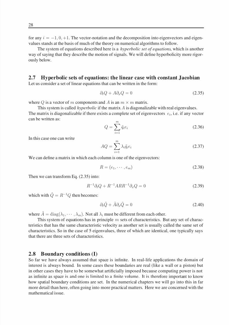
Figure 2.2. Characteristics of Burger’s equation. Left: case of diverging characteristics. Right:

case of converging characteristics with the formation of a singularity. Beyond the time of the

creation of the singularity the solution is ill defined unless a recipe is given how to treat the

singularity.

where ∂F ∂Q

is the Jacobian matrix, which depends, in the non-linear case, on Q itself. We can

nevertheless decompose this matrix in eigenvectors (which depend on Q) and we obtain

∂ tQ +

λ1

. . .

λm

∂ xQ = 0 (2.56)

Here the eigenvalues λ1, · · · , λm and eigenvectors (and hence the meaning of Q) depends on Q.

In principle this is not a problem. The characteristics are now simply given by the state vector Qitself. The state is, so to speak, self-propagating. We are now getting into the kind of hyperbolic

equations like the hydrodynamics equations, which are also non-linear self-propagating.

2.13 Example of non-linear conservation equation: Burger’s equationConsider

∂ tq +1

2∂ x(q2) = 0 (2.57)

This is called Burger’s equation. It is a conservation equation in q, with flux f (q) = q2/2. The

flux is only dependent on x through q. We have ∂f/∂q = q, so we can write the above equation

as

∂ tq + q∂ xq = 0 (2.58)

So the advection velocity is, in this important example, the to-be-advected quantity q itself! The

quantity propagates itself with u = q. If we use the comoving derivative, then we obtain the

following equation:

Dtq(x, t) = 0 (2.59)

which appears to be identical to Eq. (2.8). The difference lies in the definition of Dt which is

defined with respect to a given function u(x) in Eq. (2.8) and with respect to q(x, t) in Eq. (2.59).

Eq. (2.59) shows that along a characteristic the value of q does not change, or in other

words: the characteristic speed (slope in the x, t-plane) does not change along a characteristic.

This means that the characteristics are straight lines in the (x, t)-plane, as in the case of the

example of Section 2.3. The difference to that example lies in the fact that in this case not all

straight line characteristics are parallel.

The interpretation of Burger’s equation is that of the motion of a pressureless fluid . Often

it is said to be the equation describing the motion of dust in space, as dust clouds do not have



33

pressure and each dust particle moves along a straight line. This is only partially correct, as we

shall show below, but it does describe roughly the point.

Since any non-parallel straight lines in (x, t) must have a crossing at some point in space

we can immediately derive that for converging flows there will be a point at which Burger’s

equations break down.

Now to come back at the difference of Burger’s equation with the motion of dust. In

Burger’s equation the assumption is that at any time and any position there exists only one ve-

locity. In case of dust flows this is not necessary: since the particles do not interact, at any given

time and position one can have dust particles flowing left, right at various velocities. If two

dust cloud approach, in Burger’s equation the equations produce shocks (i.e. a breakdown of the

pure inviscid equation). In the case of dust the particles would not feel each other and the cloud

simply go through each other.

Perhaps a more adequate physical interpretation of Burger’s equation is that of a pressure-

less fluid. If the characteristics converge a shock will happen and Burger’s equation will no

longer be valid and will be replaced by the more generally valid hydrodynamics equation with

pressure.

→ Exercise: As we have shown in Section 2.3 a conserved quantity tends to grow in regions

of converging flow and it tends to diminish in regions of diverging flow. In case of Burger’s

equation it appears that this is not the case, as the equation amounts to Dtq = 0. Give a

modified version of Burger’s equation that does have this property of increasing value for

converging flow, and note which is the characteristic speed.

2.14 Isothermal hydrodynamic equationsThe topic of this lecture is hydrodynamics, so let’s express the equations of hydrodynamics in

the above form. Let’s take the isothermal equations for simplicity. We have

∂ tρ + ∂ x(ρu) = 0 (2.60)

∂ t(ρu) + ∂ x(ρu2 + ρc2s) = 0 (2.61)

Let us define

q1 ≡ ρ , q2 ≡ ρu (2.62)

Then we can write the above equations as

∂ t

q1q2

+ ∂ x q2

q22

q1+ q1c2s

= 0 (2.63)

or in other words: Q = (q1, q2) and F = (q2, q22/q1+q1c2s). This can be written with the Jacobian:

∂ t

q1q2

+

0 1

c2s − q22

q21

2 q2q1

∂ x

q1q2

= 0 (2.64)

The eigenvalues are

λ± =q2q1± cs = u ± cs (2.65)

and the eigenvectors are:e± =

1

λ±

(2.66)



34

One sees that both the eigenvalues and the eigenvectors depend on the state vector (q1, q2) itself

and are therefore space- and time-dependent. The state vector determines for itself how it should

be decomposed. Modes mix in two different ways: a) the eigenvectors change in space and time,

and b) each mode influences the other mode due to the non-linearity.

→ Exercise: In Section 2.6 we derived the set of eigenvectors and eigenvalues for the pertur-

bation equation of hydrodynamics with an adiabatic equation of state. If we replace γP 0/ρ0with the isothermal sound speed c2s , then we obtain the results for isothermal waves. The

funny thing is, however, that the Jacobain matrix in that case (Eq. 2.23) does not appear to

be the linearized form of the Jacobian matrix derived in the present section (the one used in

Eq. 2.64). Explain this in terms of how the linearization is done in Section 2.6.

2.15 Non-isothermal hydrodynamic equations

Now let us turn to the generalization of the isothermal hydrodynamics equations: the non-isothermal hydrodynamics equations. Note that this is not equal to the adiabatic hydrodynamics

equations, because the adiabatic hydrodynamics equations assume that all of the gas lies on the

same adiabat, or in other words: that the gas is isentropic. In constrast, we would now like to

relax any assumption of the entropy of the gas, and allow the entropy of the gas to vary arbitrar-

ily in space. This means necessarily that we must include a third equation: the energy equation.

Now the equations become significantly more complex.

We have now:

∂ tρ + ∂ x(ρu) = 0 (2.67)

∂ t(ρu) + ∂ x(ρu2 + P ) = 0 (2.68)

∂ t(ρetot) + ∂ x[(ρetot + P )u] = 0 (2.69)

Let us define

q1 ≡ ρ , q2 ≡ ρu , q3 ≡ ρetot (2.70)

Then we can write the above equations as

∂ t

q1

q2q3

+ ∂ x

f 1

f 2f 3

= 0 (2.71)

in which

f 1f 2f 3

= ρu

ρu2 + P (ρetot + P )u

=

q2

(γ − 1)q3 +3−γ 2

q2

2

q1

γ q3q2q1

+1−γ 2

q32

q21

(2.72)

where we used

u = q2/q1 (2.73)

P = (γ − 1)

q3 − 1

2

q22q1

(2.74)

Eq. 2.71 with the above expressions for (f 1, f 2, f 3) can be written with the Jacobian:

∂ tq1

q2q3

+

0 1 0

γ −32

q22q1 (3 − γ ) q

2

q1 (γ − 1)−

γ q3q2q21

+ (γ − 1) q3

2

q31

γ q3q1

+ 32

(1 − γ ) q2

2

q21

γ q2q1

∂ xq1

q2q3

= 0 (2.75)



35

It can be useful to rewrite the Jacobian using the primitive variables:

∂ tq1q2q3 +

0 1 0γ −32

ρu2 (3

−γ )u (γ

−1)

−{γetotu + (γ − 1)u3} γetot + 3

2(1 − γ )u2

γu ∂ x

q1q2q3 = 0

(2.76)

The eigenvalues are

λ− = u− C s (2.77)

λ0 = u (2.78)

λ+ = u + C s (2.79)

(2.80)

with eigenvectors:

e− =

1

u − C shtot − C su

(2.81)

e0 =

1

u12

u2

(2.82)

e+ =

1

u + C shtot + C su

(2.83)

where htot = etot + P/ρ is the total specific enthalpy and C s =

γP/ρ is the adiabatic sound

speed.

2.16 Traffic flow equationsAs already mentioned, hyperbolic equations are more general than only the equations of hydro-

dynamics. Here is an example of a model of traffic flow, as was first discussed in papers by

Lighthill, Whitham and Richards ( for the references, see book LeVeque from which this exam-

ple is taken). Let us assume a single lane road with a density of cars q (the number of cars per

car length). We assume that 0 ≤ q ≤ 1 (because we cannot have more than 1 car per car length)and we verify a-posteriori if this condition is satified. The conservation equation is:

∂ tq + ∂ x(qu) = 0 (2.84)

where u is the speed of the cars at time t and position x. Suppose that there is a speed limit of

umax and that if the road is nearly empty, the cars drive at the speed limit u = umax. If this was all,

then the advection equation simply moves the density of cars linearly toward larger x. However,

if the road gets more crowded drivers naturally slow down. Let us for simplicity assume that

u(q) = umax(1 − q) (2.85)

The flux of cars is then

f = q(1 − q)umax (2.86)



36

The flux of cars is greatest when q = 1/2. For lower q the flux is lower because the density

of cars is lower, while for higher q the flux is lower because the speed of the cars goes down

(congestion).

We can now write the traffic flow equation as

∂ tq + umax(1 − 2q)∂ xq = 0 (2.87)

This shows that the characteristic velocity of the system is:

λ = umax(1 − 2q) (2.88)

which can range from −umax to umax. It is very important to note here that the characteristic

speed is not equal to the speed of propagation of the cars! It is the speed at which information is

propagating, not the speed of the advected quantity q itself. This is one of the peculiar features

of non-linear hyperbolic equations, and it is very similar to the peculiarities of the Burger’sequation. The traffic flow equation is a particularly nice example of a non-linear hyperbolic

equation because it is a very simple equation, yet has very interesting solution properties.

2.17 Hyperbolic equations in 2-D and 3-DSo far we have done everything only in 1-D. But what we learned can also be generalized to

higher dimensions, by use of the concept of operator splitting. In 2-D we get

∂ tQ + ∂ xF (Q) + ∂ yG(Q) (2.89)

which can be written as:

∂ tqi +∂f i∂qk

∂ xqk +∂gi

∂qk∂ yqk (2.90)

By operator splitting we can focus our attention to one of the space dimensions only. If we split

it as

∂ tqi +∂f i∂qk

∂ xqk = −∂f i∂qk

∂ yqk (2.91)

then we focus on the advection in x-direction, and consider the y-advection as a source term,

while if we write

∂ tqi +∂f i

∂qk∂ yqk =

−∂f i

∂qk∂ xqk (2.92)

we focus on advection in y-direction and consider the x-direction as a source term. In numer-

ical methods this operator splitting is often done to reduce the full 2-D or 3-D problem into

consecutive 1-D problems which are much easier to handle.

Documents

Chap 2 Hyperbolic