CHAOTIFYING FUZZY HYPERBOLIC MODEL USING ADAPTIVE INVERSE ... · October 27, 2004 17:48 01144 Chaotifying Fuzzy Hyperbolic Model Using Adaptive Inverse Optimal Control Approach 3507

October 27, 2004 17:48 01144

International Journal of Bifurcation and Chaos, Vol. 14, No. 10 (2004) 3505–3517c© World Scientific Publishing Company

CHAOTIFYING FUZZY HYPERBOLIC MODEL

USING ADAPTIVE INVERSE OPTIMAL

CONTROL APPROACH*

HUAGUANG ZHANG† and ZHILIANG WANG‡

School of Information Science and Engineering, Northeastern University,

Shenyang, Liaoning 110004, P. R. China†hg [email protected]

‡wang zhi [email protected]

DERONG LIUDepartment of Electrical and Computer Engineering,

University of Illinois at Chicago,

Chicago, IL 60607-7053, USA

[email protected]

Received March 21, 2003; Revised September 25, 2003

In this paper, the problem of chaotifying the continuous-time fuzzy hyperbolic model (FHM)is studied. By tracking the dynamics of a chaotic system, a controller based on inverse optimalcontrol and adaptive parameter tuning methods is designed to chaotify the FHM. Simulationresults show that for any initial value the FHM can track a chaotic system asymptotically.

Keywords : Chaotification; fuzzy hyperbolic model; adaptive inverse optimal control.

1. Introduction

It is well known that most conventional controlmethods and many special techniques can be usedfor chaos control [Chen & Dong, 1998] whether thepurpose is to reduce “bad” chaos or to introduce“good” chaos. Numerous control methodologieshave been proposed, developed, tested and applied.Due to its great potential in nontraditional ap-plications such as those found within the contextof physical, chemical, mechanical, electrical, opti-cal and particularly, biological and medical systems[Schiff et al., 1994; Yang et al., 1995], making anonchaotic system chaos or strengthening the ex-isting chaos, known as “chaotification” (also knownas “anticontrol”), has attracted increasing atten-

tion in recent years. The process of chaos controlis now understood as a transition from chaos toorder and sometimes from order to chaos, depend-ing on the purpose of the application in differentcircumstances.

Recent studies have shown that any discretemap can be chaotified in the sense of Devaneyor Li–Yorke by a state-feedback controller witha uniformly bounded control-gain sequence de-signed to make all Lyapunov exponents of thecontrolled system strictly positive or arbitrarilyassigned [Chen & Lai, 1997; Chen & Lai, 1998;Wang & Chen, 1999, 2000a, 2000b, 2000c]. Evenif there are some research works showing that aclass of continuous stable systems can be chaotified

∗This work was supported by the National Natural Science Foundation of China (60325311, 60274017).†Author for correspondence.

3505

October 27, 2004 17:48 01144

3506 H. Zhang et al.

[Wang et al., 2000; Wang et al., 2001; Tang et al.,2001; Sanchez et al., 2001; Zhong et al., 2001; Yanget al., 2002; Lu et al., 2002], the problem how tochaotify general nonlinear systems that cannot belinearized is still unsolved.

A systematic design procedure, the fuzzy con-trol method, has been widely used to control chaoticsystems. Great success has been achieved in vari-ous applications especially in situations where thedynamics of systems are so complex that it is im-possible to construct an accurate model [Passino &Yurkovich, 1998; Tanaka et al., 1998; Chen & Chen,1999; Chen et al., 1999]. In the present work westudy the chaotification of a specific fuzzy model.First, such a study is of academic interest sincea fuzzy model is usually a nonlinear system andits chaotification is a difficult task in general. Sec-ond, to obtain a chaotic fuzzy model, the com-mon method is to use fuzzy modeling approach tomodel a chaotic system [Tanaka et al., 1998; Chenet al., 1999]. On the other hand, it is natural to askwhether a nonchaotic fuzzy system can be chaoti-fied by control inputs. Part of the answer has beengiven in [Li et al., 2002] where the continuous-timeT-S fuzzy model was chaotified under certain con-ditions. Parallel to the T-S fuzzy model, a newcontinuous-time fuzzy model, called the fuzzy hy-perbolic model (FHM), has recently been proposed[Zhang & Quan, 2001; Quan, 2001]. When mod-eling a complex plant, an FHM can be obtainedwithout knowing much information about the realplant, and it is easy to design a controller with anFHM since the FHM satisfies the Lipschitz con-dition. In this paper, we focus on how to makean FHM chaotified. In fact, the FHM belong toa class of Lur’e systems. The problem of robustH∞ synchronization of two Lur’e systems has beenstudied in [Suykens et al., 1997; Suykens et al.,1997; Suykens et al., 1999]. In these studies, suf-ficient conditions for uniform synchronization with

a bound on the synchronization error were derivedin the form of matrix inequalities, and the prob-lem of controller design is solved using a nonlinearoptimization approach. The merits of these resultsare that the structures of the controllers are sim-ple, and relatively large parameter mismatches areallowed such that the systems remain synchronizedwith a relatively small synchronization error bound.However, since the controllers are not adaptive, syn-chronization errors will not converge to zero. Inour approach, for a controlled FHM to track thedynamics of a given continuous-time chaotic sys-tem asymptotically, we design a controller directlywithin the framework of inverse optimal control the-ory with adaptive parameter tuning methods. Byusing inverse optimal control theory, we guaranteethat the controller is optimal with a meaningful costfunctional, and by using adaptive parameter tuningmethods, we make the tacking errors converge tozero asymptotically.

This paper is organized as follows. In Sec. 2,preliminaries about the FHM are reviewed. InSec. 3, the problem considered in this paper is de-scribed. In Sec. 4, a controller that can chaotify theFHM is designed. Simulation results are presentedin Sec. 5, and conclusions are given in Sec. 6.

2. Preliminaries

In this section we review some necessary prelimi-naries for the FHM.

Definition 1. Given a plant with n input vari-ables x = (x1(t), . . . , xn(t))T and n output variablesx = (x1(t), . . . , xn(t))T . If each output variable cor-responds to a group of fuzzy rules which satisfiesthe following conditions:

(i) For each output variable xl, l = 1, 2, . . . , n,the corresponding group of fuzzy rules has thefollowing form:

Rj : IF x1 is Fx1, x2 is Fx2

, . . . , and xnlis Fxnl

THEN xl = c±Fx1

+ c±Fx2

+ · · · + c±Fxnl

, j = 1, . . . , 2nl ,

where Fxi(i = 1, . . . , nl) are fuzzy sets of xi, which

include Pxi(positive) and Nxi

(negative), and c±Fxnl

(i = 1, . . . , nl) are 2nl real constants correspondingto Fxi

;(ii) The constant terms c±Fxi

in the THEN-

part correspond to Fxiin the IF-part; that is, if

the language value of Fxiterm in the IF-part is Pxi

,c+Fxi

must appear in the THEN-part; if the language

value of Fxiterm in the IF-part is Nxi

, c−Fxi

must

appear in the THEN-part; if there is no Fxiin the

IF-part, c±Fxi

does not appear in the THEN-part;

October 27, 2004 17:48 01144

Chaotifying Fuzzy Hyperbolic Model Using Adaptive Inverse Optimal Control Approach 3507

(iii) There are 2nl fuzzy rules in each rule base;that is, there are a total of 2nl input variable com-binations of all the possible Pxi

and Nxiin the

IF-part.

We call this group of fuzzy rules “hyperbolictype fuzzy rule base” (HFRB). To describe a plantwith n output variables, we will need n HFRBs.

Theorem 1 [Quan, 2001; Zhang & Quan, 2001].Given n HFRBs, if we define the membership

function of Pxiand Nxi

as:

µPxi(xi) = e−

1

2(xi−ki)

2

µNxi(xi) = e−

1

2(xi+ki)

2(1)

where i = 1, . . . , n and ki are constants. Denoting

c+Fxi

by cPxiand c−Fxi

by cNxi, we can derive the fol-

lowing model:

xl = f(x)

=

nl∑

i=1

cPxiekixi + cNxi

e−kixi

ekixi + e−kixi

=

nl∑

i=1

pi +

nl∑

i=1

qiekixi − e−kixi

ekixi + e−kixi

=

nl∑

i=1

pi +

nl∑

i=1

qi tanh(kixi) (2)

where

pi =cPxi

+ cNxi

2and qi =

cPxi− cNxi

2.

Therefore, the whole system has the following form:

x = P + A tanh(Kx) (3)

where P is a constant vector, A is a constant matrix,and tanh(Kx) is defined by

tanh(Kx) = [tanh(k1x1), tanh(k2x2), . . . , tanh(knxn)]T .

We will call (3) a fuzzy hyperbolic model(FHM).

Let Y be the space composed of all the func-tions having the form of the right-hand side of (2).We then have the following theorem.

Theorem 2. For any given real continuous g on

the compact set U ⊂ Rn and arbitrary ε > 0, there

exists an f ∈ Y such that

supx∈U

|g(x) − f(x)| < ε .

Proof. See Appendix A. �

From Definition 1, if we set cPxiand cNxi

neg-ative to each other, we can obtain a homogeneousFHM:

x = A tanh(Kx) . (4)

The homogeneous FHM given in (4) will bestudied in this paper for chaotification through theuse of an adaptive controller.

3. Problem Description

Since the difference between (3) and (4) is only theconstant vector term in (3), there is essentially nodifference between the control of (3) and (4). In thissection, we will design a fuzzy controller for homo-geneous FHM that can chaotify the model in (4).

Suppose that there exists a chaotic system hav-ing the following form:

xr = fr(xr), xr ∈ Rn, fr(·) ∈ Rn . (5)

Consider an uncontrolled FHM in the followingform:

x = Af(x) = A tanh(Kx) (6)

where x is the state and A = [aij ]n×n is a ma-trix. Due to the hyperbolic tangent form of f(x),we know that fT (x) · x ≥ 0 for all x, f(x) = 0 onlyat x = 0, and lim‖x‖2→∞ fT (x) · x = +∞. There-fore, there exist positive constants γ1 and γ2 suchthat γ1‖x‖

22 ≤ fT (x) · x ≤ γ2‖x‖

22 [Miller & Michel,

1982].The idea here is to design a controller u such

that the controlled FHM

x = Af(x) + u , (7)

can track the dynamics of system (5), i.e.

limt→∞

‖e(t)‖2 = limt→∞

‖x(t) − xr(t)‖2 = 0 . (8)

For each output xl, l = 1, . . . , n, we choose to usethe following controller fuzzy rule base (CFRB):

Ri : IF x1 is Fx1, x2 is Fx2

, . . . , and xnlis Fxnl

THEN ul = uil(x) i = 1, . . . , 2nl

That is to say, each CFRB has the same IF-partas that of the corresponding HFRB, and has eachTHEN-part given by a nonlinear function of theplant’s state. By this design method, we get acontroller as

u(x) = [u1(x), u2(x), . . . , un(x)]T , (9)

October 27, 2004 17:48 01144


where

ul =

2nl∑

i=1

hil(x)ui

l(x), l = 1, . . . , n (10)

and

hil(x) =

nl∏

k=1

µiFx

k

/

2nl∑

i=1

nl∏

k=1

µiFx

k

. (11)

In (11), µiFx

k

is the membership function of Fxkwith

the ith rule. It is easy to see that

2nl∑

i=1

hil(x) = 1 . (12)

Adding this controller to (6), we obtain the con-trolled system (7).

Suppose that u has the form u(x, t) = v(x) +w(x, t), where v(x) = Λx is the state-feedback,Λ = −diag[λi]n×n ∈ Rn×n with λi (i = 1, . . . , n)real numbers, and w(x, t) is to be designed. Then,(7) becomes

x = Λx + Af(x) + w(x, t) . (13)

From (5) and (13), we obtain

e = Λx + Af(x) + w(x, t) − fr(xr) . (14)

In practical control applications, since Λ is thestate-feedback matrix and A is determined by thefuzzy rules, they may be affected by some uncer-tain factors such as parameter shifts and errors inmodeling, and therefore, the parameters of system(14), Λ and A, would include some uncertainties. Onthe other hand, ki (i = 1, . . . , n) can be fixed sincethey are determined by the membership functionschosen in modeling. Once the membership func-tions are fixed, ki (i,= 1, . . . , n) are invariant. Soin this paper, we assume Λ and A are tunable, andki (i = 1, . . . , n) are constants.

For system (13) to track the system (5), thefollowing natural solvability assumption is needed[Li & Krstic, 1997].

Assumption 1. There exist functions ρ(t) andα(t) such that

dρ(t)

dt= Λ0ρ(t) + A0f(ρ(t)) + α(t)

ρ(t) = xr(t)

(15)

where A0 = [a0ij ]n×n and Λ0 = −diag[λ0i]n×n areknown constant matrices and λ0i are positive realnumbers for i = 1, . . . , n.

From (5) and (15) the following equation canthen be derived:

Λ0xr + A0f(xr) + α(t) = fr(xr) . (16)

Substituting (16) into (14), we have

e = Λ0e + A0[f(e + xr) − f(xr)]

+[w − α(t)] + Λx + Af(x) (17)

where Λ = Λ − Λ0 = −diag[λi − λ0i]n×n andA = A − A0 = [aij − a0ij ]n×n = [aij ]n×n. Letφ(e, xr) = f(e + xr) − f(xr), u = w − α(t). Then,(17) can be rewritten as

e = Λ0e + A0φ(e, xr) + Λx + Af(x) + u . (18)

Remark 1. It is clear that φ(e, xr) = 0 if e = 0.Moreover, f(e + xr) = A tanh(K(e + xr)) is mono-tonically increasing (or decreasing) for each com-ponent ei of e. Since ei > 0 (or ei < 0) impliesthat ei + xri > xri (or ei + xri < xri) for all xri,fi(ei +xri) > fi(xri) (or fi(ei +xri) < fi(xri)). Thismeans that φT (e, xr)e = (f(e + xr)− f(xr))

T e > 0.Therefore, there exist positive constants γ1, γ2, andLφ such that

γ1‖e‖22 ≤ φT (e, xr)e ≤ γ2‖e‖

22 (19)

and

‖φ(e, xr)‖2 < Lφ‖e‖2 . (20)

Therefore, φ(e, xr) is Lipschitz with respect to e.

4. Controller Design

We first state the following lemma that is requiredin our controller design.

Lemma 4.1 [Sanchez, 2001]. For all matrices X,Y ∈ Rn×k and Q ∈ Rn×n with Q = QT > 0, the

following inequality holds:

XT Y + Y T X ≤ XT QX + Y T Q−1Y . (21)

Theorem 3. For system (14 ), if the controller is

chosen as

w = −(AT0 A0 + I)φ(e, xr) − Λ0xr

− A0f(xr) + fr(xr) (22)

October 27, 2004 17:48 01144


and the parameter adaptive update laws are chosen

as

λi = −φi(e, xr)xi ,

aij = −φi(e, xr)fj(x) ,(23)

for i = 1, . . . , n, j = 1, . . . , n, in which φi(e, xr)and xi are the ith component of φ(e, xr) and x,respectively, and fj(x) is the jth component of f(x),then the state of system (18 ), e, is globally asymp-

totically stable, i.e.

limt→∞

‖e(t)‖2 = 0 .

Proof. Using (16), we can get α(t) = fr(xr) −Λ0xr − A0f(xr). Thus,

u = w(x, t) − α(t)

= −(AT0 A0 + I)φ(e, xr) . (24)

Define

ε∆= [eT (t), θT (t)]T

= [eT (t), λ1(t), . . . , λn(t), a11(t), . . . ,

a1n(t), a21(t), . . . , ann(t)]T .

We choose

V (ε) =

n∑

i=1

∫ ei

0φi(η, xr)dηi

+1

2

n∑

i=1

λ2i +

1

2

n∑

i=1,j=1

a2ij , (25)

where ηi is the ith element of η.Because of (19), we know that V (ε) is radially

unbounded, i.e. V (ε) > 0 for all ε and V (ε) → ∞as ‖ε‖2 → ∞. Its time-derivative is as follows:

V (ε) = φT (e, xr)(Λ0e + A0φ(e, xr)

+ Λx + Af(x) + u)

+

n∑

i=1

λiλi +

n∑

i=1,j=1

aijaij

= φT (e, xr)Λ0e + φT (e, xr)A0φ(e, xr)

+ φT (e, xr)(Λx + Af(x))

+ φT (e, xr)u +

n∑

i=1

λiλi +

n∑

i=1,j=1

aij aij

∆= LfV + (LgV )u (26)

where

LfV∆= φT (e, xr)Λ0e + φT (e, xr)A0φ(e, xr)

+ φT (e, xr)(Λx + Af(x))

+n∑

i=1

λiλi +n∑

i=1,j=1

aijaij (27)

and

LgV∆=φT (e, xr) . (28)

Applying Lemma 1 with Q = I, we get

V (ε) = φT (e, xr)Λ0e +1

2φT (e, xr)φ(e, xr)

+1

2φT (e, xr)A

T0 A0φ(e, xr)

+ φT (e, xr)u + φT (e, xr)(Λ(t)x

+ A(t)f(x)) +

n∑

i=1

λiλi +

n∑

i=1,j=1

aij aij

= φT (e, xr)Λ0e +1

2φT (e, xr)φ(e, xr)

+1

2φT (e, xr)A

T0 A0φ(e, xr) + φT (e, xr)u

+

n∑

i=1

λi(λi + φi(e, xr)xi)

+n∑

i=1,j=1

aij(aij + φi(e, xr)fj(x)) .

Substituting (23) into the equality above and usinginequalities (19) and (20), we obtain

V (ε) ≤ −

(

λ∗γ1 −1

2L2

φ

)

‖e‖22

+1

2φT (e, xr)A

T0 A0φ(e, xr)

+ φT (e, xr)u (29)

where λ∗ = min{λ0i; i = 1, . . . , n}.If we let R−1(ε) = (1/β)(AT

0 A0 + I), whereβ ≥ 2 is a constant, we have

−βR−1(ε)(LgV )T = u

= −(AT0 A0 + I)φ(e, xr) . (30)

In general R−1(ε) is a function of ε, but for ourpurpose it is chosen as a constant matrix. The mo-tivation for this operation will be seen from theinverse optimization problem to be discussed later.

October 27, 2004 17:48 01144


Substituting (24) into (29), we get

V (ε) ≤ −

(

λ∗γ1 −1

2L2

φ

)

‖e‖22

−1

2‖AT

0 A0‖L2φ‖e‖

22 − L2

φ‖e‖22

= −

(

λ∗γ1 +1

2‖AT

0 A0‖L2φ +

1

2L2

φ

)

‖e‖22

≤ 0 . (31)

By LaSalle’s invariance principle [Slotine & Li,1991], we know that the invariant set of (15), IS,has the following form:

IS = {ε|V = 0} = {ε|(0, θT )} .

This completes the proof of the theorem. �

Remark 2. From the proof of Theorem 3, we canfind that even in the case limt→∞ ‖e(t)‖2 = 0, thelimits limt→∞ ‖Λ(t)‖2 and limt→∞ ‖A(t)‖2 may notbe zero. This conclusion can also be drawn from(23), from which we get φ(e, xr) = 0 if e = 0. Thisimplies that Λ(t) and A(t) approach some constantswhich may be different from Λ0 and A0.

To avoid the burden that the partial differen-tial equation of Hamillton–Jacobi–Bellman (HJB)imposes on the problem of optimal control of non-linear systems, inverse optimal control theory hasbeen developed recently. The difference between thetraditional optimization and inverse optimal con-trol problem is that, the former seeks a controllerthat minimizes a given cost, while the latter isconcerned with finding a controller that minimizessome “meaningful” cost.

According to Li and Krstic [1997] and Krsticand Li [1998], for the inverse optimal control prob-lem of system (18) to be solvable under the controlof (23) and (24) we need to find a positive real-valued function R(ε) and a positive definite func-tion l(ε) such that the following cost functional

J(u) = limt→∞

{2βV (ε(τ)) +

∫ t

0(l(ε(τ))

+ u(τ)T R(ε(τ))u(τ))dτ}, β ≥ 2 (32)

is minimized.In the following, we will show that the con-

troller we have designed can indeed solve the inverseoptimal control problem.

Theorem 4. If we choose

l(ε) = −2βLfV + 2β(LgV )R−1(ε)(LgV )T

+ β(β − 2)((LgV )R−1(ε)(LgV )T )

= −2βLfV + β2(LgV )R−1(ε)(LgV )T (33)

and

R(ε) = β(AT0 A0 + I)−1 , β ≥ 2 , (34)

the cost functional (32 ) for system (18 ) under the

parameter update laws (23 ) and the state feedback

law (24 ) will be minimized.

Proof. To prove this theorem, first we should provethat R(ε) is positive and symmetry, and l(ε) is radi-ally unbounded, i.e. R(ε) = RT (ε) > 0 and l(ε) > 0for all ε 6= 0 and l(ε) → +∞ as ε → ∞. It is clearthat R(ε) chosen according to (34) satisfies this re-quirement. Using (23), (24), (27), (28), and (34), weobtain

l(ε) = 2βφT (e, xr)Λ0e − 2βφT (e, xr)A0φ(e, xr)

+βφT (e, xr)(AT0 A0 + I)φ(e, xr) . (35)

Applying Lemma 1 to the second term on the right-hand side of (35), we get

l(ε) ≥ 2βλ∗φT (e, xr)e − βφT (e, xr)φ(e, xr)

− βφT (e, xr)AT0 A0φ(e, xr)

+ βφT (e, xr)(AT0 A0 + I)φ(e, xr)

≥ 2βλ∗φT (e, xr)e . (36)

This means that l(ε) is radially unbounded. Substi-tuting (30) into (26), we get

V = LfV + (LgV )(−βR−1(ε))(LgV )T . (37)

Multiplying it by −2β, we obtain

−2βV (ε(t)) = −2βLf V

+ 2β2(LgV )R−1(ε)(LgV )T . (38)

Considering (30) and (33), we get

l(ε) + uT R(ε)u = −2βV (ε(t)) . (39)

Substituting (39) into (32), we have

J(u) = limt→∞

{

2βV (ε(t)) +

∫ t

0−2βV (ε(τ))dτ

}

= limt→∞

{2βV (ε(t)) − 2βV (ε(t)) + 2βV (ε(0))}

= 2βV (ε(0)) . (40)

October 27, 2004 17:48 01144


Thus, the minimum of the cost functional is J(u) =2βV (ε(0)) for the optimal control law (23) and (24).The theorem is proved. �

We now summarize the results presented abovein the next theorem.

Theorem 5. If we choose feedback control law u =v + w in which v = Λx is the linear state feed-

back with Λ a diagonal constant matrix and w =−(AT

0 A0 + I)φ(e, xr) − Λ0xr − A0f(xr) + fr(xr) is

the nonlinear feedback, and at the same time we

choose parameter update laws for Λ and A according

to (23 ), the controlled FHM (7 ) will be chaotified

through minimizing the cost functional (32).

Remark 3. Here, we should note that the designedcontroller is not unique since we have much free-dom to select Λ0 and A0. In fact, it is necessaryto select proper Λ0 and A0 so that the controller’senergy satisfies requirements in practical applica-tions. Once Λ0 and A0 are fixed, the controller isoptimal which minimizes some “meaningful” cost.Theorem 5 also indicates that we can use FHM as ageneral device to produce various chaotic dynamics.

In practice, the control signal ul(x) in (10) isdefined by ui

l(x) (i = 1, . . . , 2nl ; l = 1, . . . , n). Solu-tions for ui

l in (10) are not unique since there are 2nl

unknown variables to be solved from only one equa-tion. In our study, we use a heuristic approach. Thatis, suppose for each l = 1, . . . , n, ui

l(x) = uil ∈ [ai

l , bil]

(i = 1, . . . , 2nl − 1), where uil are real numbers and

[ail , b

il] are closed intervals specified in advance. The

parameters ail and bi

l can be fixed by taking intoaccount the requirements of control signals. A spe-cial case of such solutions can be obtained wheneach ui

l(x) is equal to a nonlinear function ul(x). Inthis case, the design of a fuzzy controller becomesequivalent to the design of a normal controller.

5. Simulation Results

Suppose that we have the following HFRBs:

If x1 is Px1and x2 is Px2

, then x3 = Cx1+ Cx2

;

If x1 is Nx1and x2 is Px2

, then x3 = −Cx1+ Cx2

;

If x1 is Px1and x2 is Nx2

, then x3 = Cx1− Cx2

;

If x1 is Nx1and x2 is Nx2

, then x3 = −Cx1− Cx2

;



;



;



;



;



;



;



;



.

Here, we choose membership functions of Pxi

and Nxias follows:

µPxi(x) = e−

1

2(xi−ki)2 ,

µNxi(x) = e−

1

2(xi+ki)

2

.(41)

Then, we have the following three-dimensionalmodel:

x = Af(x) = A tanh(Kx) (42)

where x = [x1, x2, x3]T ,

A =

0 Cx2Cx3

Cx10 Cx3

Cx1Cx2

0

and tanh(Kx) = [tanh(k1x1), tanh(k2x2), tanh(k3x3)]

T .For (42), we choose the following CFRBs:


, then u3 = u13(x);


, then u3 = u23(x);


, then u3 = u33(x);


, then u3 = u43(x);


, then u2 = u12(x);


, then u2 = u22(x);


, then u2 = u32(x);


, then u2 = u42(x);


, then u1 = u11(x);


, then u1 = u21(x);


, then u1 = u31(x);


, then u1 = u41(x);

Then the controlled system is

x = Af(x) + u = Λx + Af(x) + w , (43)

where Λ = diag[λ1, λ2, λ3]. Here, because of thespecial form of A, only three adaptive update lawswill be required.

Suppose that the chaotic system we want totrack is the Lorenz system:

xr = fr(xr) (44)

where xr = [x1r, x2r, x3r]T and fr(xr) = [a(x2r −

x1r), cx1r − x1rx3r − x2r, x1rx2r − bx3r]T . When

October 27, 2004 17:48 01144


−20 −15 −10 −5 0 5 10 15 20 −40−20

020

40

0

5

10

15

20

25

30

35

40

45

50

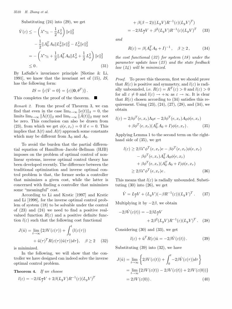
Fig. 1. Lorenz’s chaotic attractor.

−30−20

−100

1020

30 −40−20

020

400

5

10

15

20

25

30

35

40

45

50

Fig. 2. The phase diagram of (43) when the tracking object is (44).

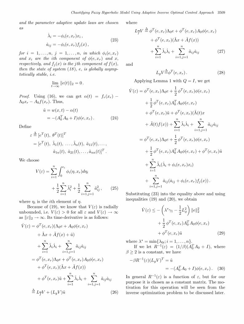
a = 10, b = 8/3, c = 28, the Lorenz system has achaotic attractor shown in Fig. 1.

In this example, we choose

Λ0 = diag[−2, −2, −2]T

Λ(0) = diag[−1, −1, −2]T ,

A0 =

0 3 4

3 0 4

3 3 0

, A(0) =

0 2.8 3.7

2.8 0 3.7

2.8 2.8 0

,

[k1, k2, k3] = [2, 3, 1]T , xr(0) = [2, 1, 3]T

and x(0) = [0, 0, 0]T . We choose these matricesin our simulation according to the following guide-lines. (1) Λ0 is a diagonal matrix with negative di-agonal elements; (2) Λ(0) is a perturbation of Λ0;(3) From the process of fuzzy modeling, we knowthat each element of matrix A0 is either positive orzero; (4) A(0) is a perturbation of A0.

The simulation results are shown in Figs. 2–4.From these figures, we can see that the controlled

October 27, 2004 17:48 01144


0 500 1000 1500 2000 2500−40

−20

0

20

40

0 500 1000 1500 2000 2500−40

−20

0

20

40

0 500 1000 1500 2000 25000

20

40

60

(a)0 500 1000 1500 2000 2500

−40

−20

0

20

40

0 500 1000 1500 2000 2500−40

−20

0

20

40

0 500 1000 1500 2000 25000

20

40

60 (b)

0 500 1000 1500 2000 2500−40

−20

0

20

40

0 500 1000 1500 2000 2500−40

−20

0

20

40

0 500 1000 1500 2000 25000

20

40

60

(c)

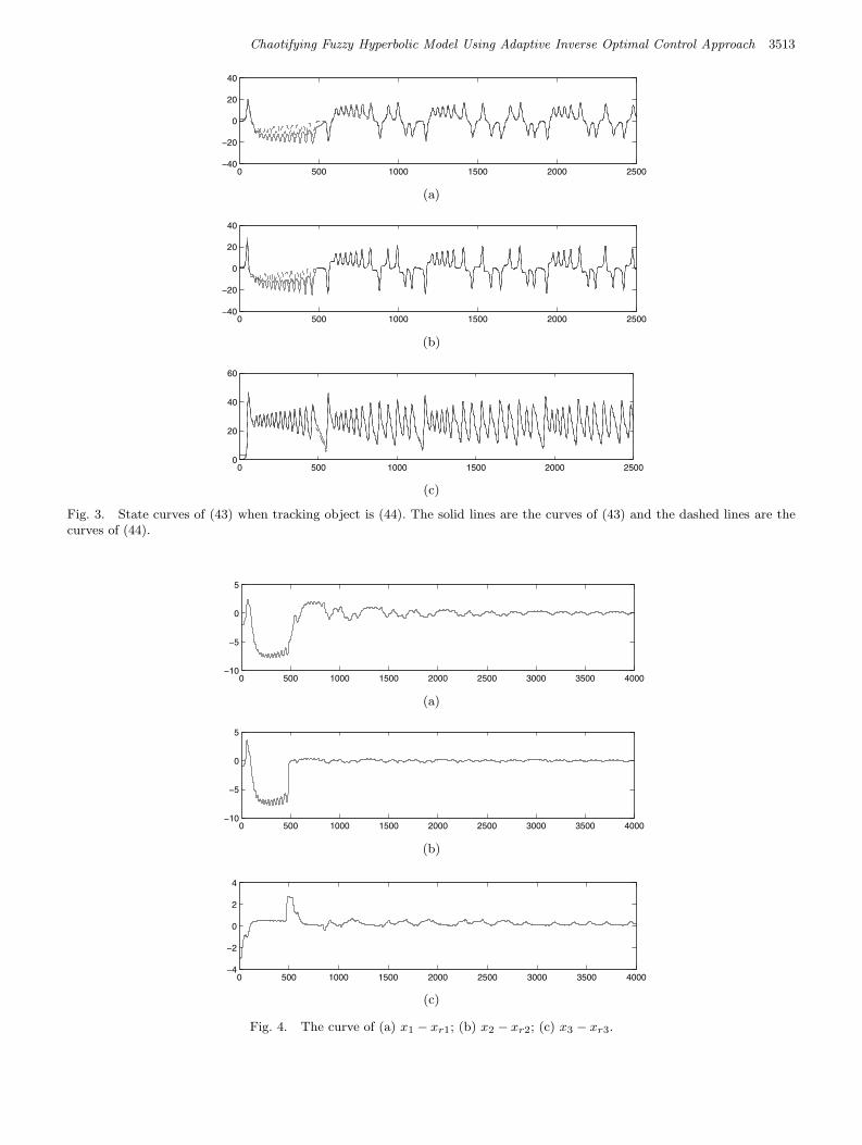
Fig. 3. State curves of (43) when tracking object is (44). The solid lines are the curves of (43) and the dashed lines are thecurves of (44).

0 500 1000 1500 2000 2500 3000 3500 4000−10

−5

0

5

0 500 1000 1500 2000 2500 3000 3500 4000−10

−5

0

5

0 500 1000 1500 2000 2500 3000 3500 4000−4

−2

0

2

4

(a)0 500 1000 1500 2000 2500 3000 3500 4000

−10

−5

0

5

0 500 1000 1500 2000 2500 3000 3500 4000−10

−5

0

5

0 500 1000 1500 2000 2500 3000 3500 4000−4

−2

0

2

4 (b)

0 500 1000 1500 2000 2500 3000 3500 4000−10

−5

0

5

0 500 1000 1500 2000 2500 3000 3500 4000−10

−5

0

5

0 500 1000 1500 2000 2500 3000 3500 4000−4

−2

0

2

4

(c)

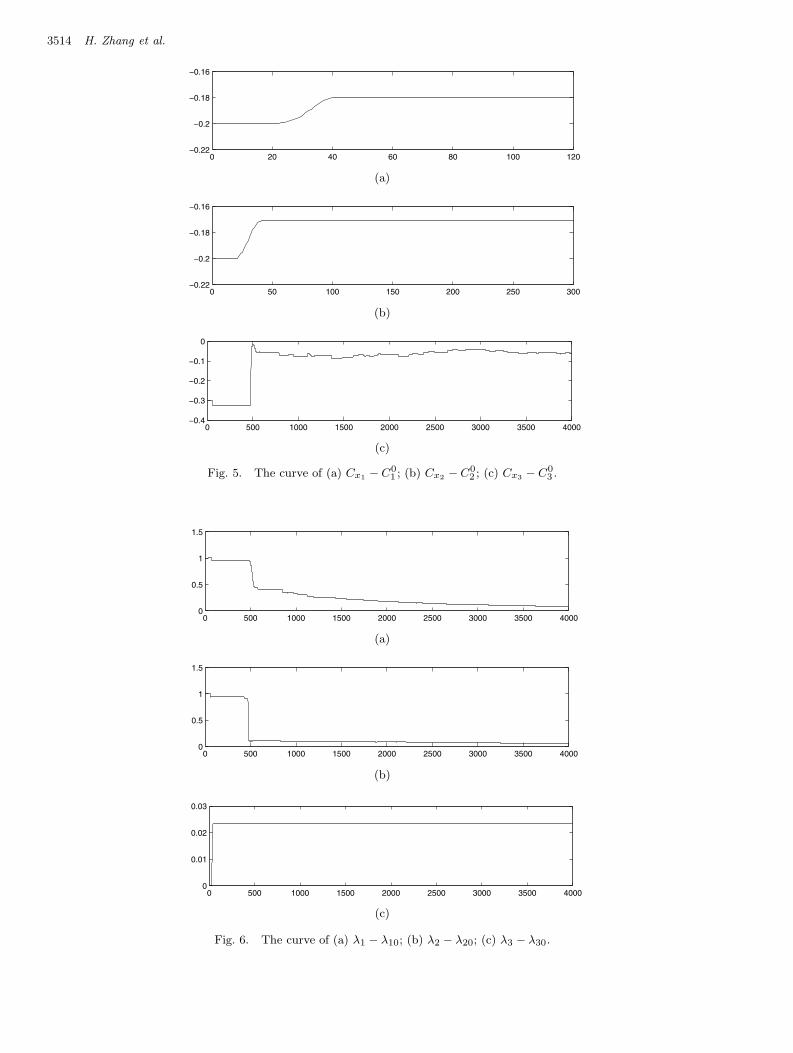
Fig. 4. The curve of (a) x1 − xr1; (b) x2 − xr2; (c) x3 − xr3.

October 27, 2004 17:48 01144


0 20 40 60 80 100 120−0.22

−0.2

−0.18

−0.16

0 50 100 150 200 250 300−0.22

−0.2

−0.18

−0.16

0 500 1000 1500 2000 2500 3000 3500 4000−0.4

−0.3

−0.2

−0.1

0

(a)0 20 40 60 80 100 120

−0.22

−0.2

−0.18

−0.16

0 50 100 150 200 250 300−0.22

−0.2

−0.18

−0.16

0 500 1000 1500 2000 2500 3000 3500 4000−0.4

−0.3

−0.2

−0.1

0 (b)

0 20 40 60 80 100 120−0.22

−0.2

−0.18

−0.16

0 50 100 150 200 250 300−0.22

−0.2

−0.18

−0.16

0 500 1000 1500 2000 2500 3000 3500 4000−0.4

−0.3

−0.2

−0.1

0

(c)

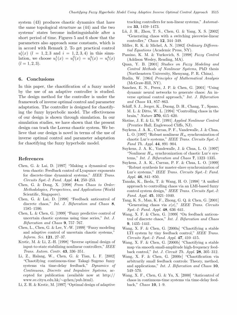
Fig. 5. The curve of (a) Cx1− C

0

1 ; (b) Cx2− C

0

2 ; (c) Cx3− C

0

3 .

0 500 1000 1500 2000 2500 3000 3500 40000

0.5

1

1.5

0 500 1000 1500 2000 2500 3000 3500 40000

0.5

1

1.5

0 500 1000 1500 2000 2500 3000 3500 40000

0.01

0.02

0.03

(a)0 500 1000 1500 2000 2500 3000 3500 4000

0

0.5

1

1.5

0 500 1000 1500 2000 2500 3000 3500 40000

0.5

1

1.5

0 500 1000 1500 2000 2500 3000 3500 40000

0.01

0.02

0.03 (b)

0 500 1000 1500 2000 2500 3000 3500 40000

0.5

1

1.5

0 500 1000 1500 2000 2500 3000 3500 40000

0.5

1

1.5

0 500 1000 1500 2000 2500 3000 3500 40000

0.01

0.02

0.03

(c)

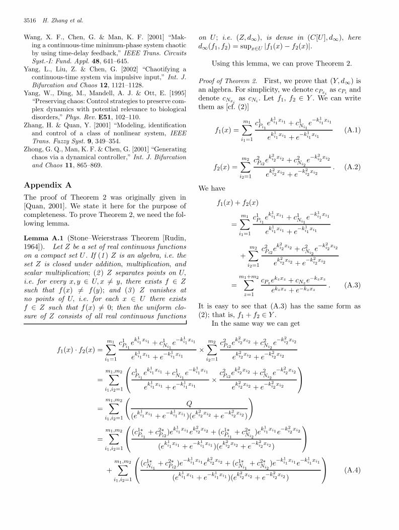
Fig. 6. The curve of (a) λ1 − λ10; (b) λ2 − λ20; (c) λ3 − λ30.

October 27, 2004 17:48 01144


system (43) produces chaotic dynamics that havethe same topological structure as (44) and the twosystems’ states become indistinguishable after ashort period of time. Figures 5 and 6 show that theparameters also approach some constants, which isin accord with Remark 2. To get practical controlui

l(x) (l = 1, 2, 3 and i = 1, 2, 3, 4) in this simu-lation, we choose u1

l (x) = u2l (x) = u3

l (x) = u4l (x)

(l = 1, 2, 3).

6. Conclusions

In this paper, the chaotification of a fuzzy modelby the use of an adaptive controller is studied.The design method for the controller is under theframework of inverse optimal control and parameteradaptation. The controller is designed for chaotify-ing the fuzzy hyperbolic model. The effectivenessof our design is shown through simulation. In oursimulation studies, we have shown that the presentdesign can track the Lorenz chaotic system. We be-lieve that our design is novel in terms of the use ofinverse optimal control and parameter adaptationfor chaotifying the fuzzy hyperbolic model.

References

Chen, G. & Lai, D. [1997] “Making a dynamical sys-tem chaotic: Feedback control of Lyapunov exponentsfor discrete-time dynamical systems,” IEEE Trans.

Circuits Syst.-I: Fund. Appl. 44, 250–253.Chen, G. & Dong, X. [1998] From Chaos to Order:

Methodologies, Perspectives, and Applications (WorldScientific, Singapore).

Chen, G. & Lai, D. [1998] “Feedback anticontrol ofdiscrete chaos,” Int. J. Bifurcation and Chaos 8,1585–1590.

Chen, L. & Chen, G. [1999] “Fuzzy predictive control ofuncertain chaotic systems using time series,” Int. J.

Bifurcation and Chaos 9, 757–767.Chen, L., Chen, G. & Lee, Y.-W. [1999] “Fuzzy modeling

and adaptive control of uncertain chaotic systems,”Inform. Sci. 121, 27–37.

Krstic, M. & Li, Z.-H. [1998] “Inverse optimal design ofinput-to-state stabilizing nonlinear controllers,” IEEE

Trans. Autom. Contr. 43, 336–351.Li, Z., Halang, W., Chen, G. & Tian, L. F. [2002]

“Chaotifying continuous-time Takagi–Sugeno fuzzysystems via time-delay feedback,” Dynamics of

Continuous, Discrete and Impulsive Systems, ac-cepted for publication (available now at http://www.ee.cityu.edu.hk/∼gchen/pub.html).

Li, Z. H. & Krstic, M. [1997] “Optimal design of adaptive

tracking controllers for non-linear systems,” Automat-

ica 33, 1459–1473.Lu, J. H., Zhou, T. S., Chen, G. & Yang, X. S. [2002]

“Generating chaos with a switching piecewise-linearcontroller,” Chaos 12, 344–349.

Miller, R. K. & Michel, A. N. [1982] Ordinary Differen-

tial Equations (Academic Press, NY).Passino, K. M. & Yurkovich, S. [1998] Fuzzy Control

(Addison Wesley, Reading, MA).Quan, Y. B. [2001] Studies on Fuzzy Modeling and

Control Methods of Nonlinear Systems, PhD thesis(Northeastern University, Shenyang, P. R. China).

Rudin, W. [1964] Principles of Mathematical Analysis

(McGraw-Hill, NY).Sanchez, E. N., Perez, J. P. & Chen, G. [2001] “Using

dynamic neural networks to generate chaos: An in-verse optimal control approach,” Int. J. Bifurcation

and Chaos 11, 857–863.Schiff, S. J., Jerger, K., Duong, D. H., Chang, T., Spano,

M. L. & Ditto, W. L. [1994] “Controlling chaos in thebrain,” Nature 370, 615–620.

Slotine, J. E. & Li, W. [1991] Applied Nonlinear Control

(Prentice Hall, Englewood Cliffs, NJ).Suykens, J. A. K., Curran, P. F., Vandewalle, J. & Chua,

L. O. [1997] “Robust nonlinear H∞ synchronization ofchaotic Lur’e systems,” IEEE Trans. Circuits Syst.-I:

Fund Th. Appl. 44, 891–904.Suykens, J. A. K., Vandewalle, J. & Chua, L. O. [1997]

“Nonlinear H∞ synchronization of chaotic Lur’e sys-tems,” Int. J. Bifurcation and Chaos 7, 1323–1335.

Suykens, J. A. K., Curran, P. F. & Chua, L. O. [1999]“Robust synthesis for master-slave synchronization ofLur’e systems,” IEEE Trans. Circuits Syst.-I: Fund.

Appl. 46, 841–850.Tanaka, K., Ikeda, T. & Wang, H. O. [1998] “A unified

approach to controlling chaos via an LMI-based fuzzycontrol system design,” IEEE Trans. Circuits Syst.-I:

Fund. Appl. 45, 1021–1040.Tang, K. S., Man, K. F., Zhong, G. Q. & Chen, G. [2001]

“Generating chaos via x|x|,” IEEE Trans. Circuits

Syst.-I: Fund. Appl. 48, 636–641.Wang, X. F. & Chen, G. [1999] “On feedback anticon-

trol of discrete chaos,” Int. J. Bifurcation and Chaos

9, 1435–1441.Wang, X. F. & Chen, G. [2000a] “Chaotifying a stable

LTI system by tiny feedback control,” IEEE Trans.

Circuits Syst.-I: Fund. Appl. 47, 410–415.Wang, X. F. & Chen, G. [2000b] “Chaotifying a stable

map via smooth small-amplitude high-frequency feed-back control,” Int. J. Circuit Th. Appl. 28, 305–312.

Wang, X. F. & Chen, G. [2000c] “Chaotification viaarbitrarily small feedback controls: Theory, method,and applications,” Int. J. Bifurcation and Chaos 10,549–570.

Wang, X. F., Chen, G. & Yu, X. [2000] “Anticontrol ofchaos in continuous-time systems via time-delay feed-back,” Chaos 10, 1–9.

October 27, 2004 17:48 01144


Wang, X. F., Chen, G. & Man, K. F. [2001] “Mak-ing a continuous-time minimum-phase system chaoticby using time-delay feedback,” IEEE Trans. Circuits

Syst.-I: Fund. Appl. 48, 641–645.Yang, L., Liu, Z. & Chen, G. [2002] “Chaotifying a

continuous-time system via impulsive input,” Int. J.

Bifurcation and Chaos 12, 1121–1128.Yang, W., Ding, M., Mandell, A. J. & Ott, E. [1995]

“Preserving chaos: Control strategies to preserve com-plex dynamics with potential relevance to biologicaldisorders,” Phys. Rev. E51, 102–110.

Zhang, H. & Quan, Y. [2001] “Modeling, identificationand control of a class of nonlinear system, IEEE

Trans. Fuzzy Syst. 9, 349–354.Zhong, G. Q., Man, K. F. & Chen, G. [2001] “Generating

chaos via a dynamical controller,” Int. J. Bifurcation

and Chaos 11, 865–869.

Appendix A

The proof of Theorem 2 was originally given in[Quan, 2001]. We state it here for the purpose ofcompleteness. To prove Theorem 2, we need the fol-lowing lemma.

Lemma A.1 (Stone–Weierstrass Theorem [Rudin,1964]). Let Z be a set of real continuous functions

on a compact set U . If (1 ) Z is an algebra, i.e. the

set Z is closed under addition, multiplication, and

scalar multiplication; (2 ) Z separates points on U,i.e. for every x, y ∈ U, x 6= y, there exists f ∈ Zsuch that f(x) 6= f(y); and (3 ) Z vanishes at

no points of U, i.e. for each x ∈ U there exists

f ∈ Z such that f(x) 6= 0; then the uniform clo-

sure of Z consists of all real continuous functions

on U ; i.e. (Z, d∞), is dense in (C[U ], d∞), here

d∞(f1, f2) = supx∈U |f1(x) − f2(x)|.

Using this lemma, we can prove Theorem 2.

Proof of Theorem 2. First, we prove that (Y, d∞) isan algebra. For simplicity, we denote cPxi

as cPiand

denote cNxias cNi

. Let f1, f2 ∈ Y . We can writethem as [cf. (2)]

f1(x) =

m1∑

i1=1

c1Pi1

ek1

i1xi1 + c1

Ni1

e−k1

i1xi1

ek1

i1xi1 + e

−k1

i1xi1

(A.1)

f2(x) =

m2∑

i2=1

c2Pi2

ek2

i2xi2 + c2

Ni2

e−k2

i2xi2

ek2

i2xi2 + e

−k2

i2xi2

. (A.2)

We have

f1(x) + f2(x)

=

m1∑

i1=1

c1Pi1

ek1

i1xi1 + c1

Ni1

e−k1

i1xi1

ek1

i1xi1 + e

−k1

i1xi1

+

m2∑

i2=1

c2Pi2

ek2

i2xi2 + c2

Ni2

e−k2

i2xi2

ek2

i2xi2 + e

−k2

i2xi2

=

m1+m2∑

z=1

cPzekzxz + cNz

e−kzxz

ekzxz + e−kzxz

. (A.3)

It is easy to see that (A.3) has the same form as(2); that is, f1 + f2 ∈ Y .

In the same way we can get

f1(x) · f2(x) =

m1∑

i1=1

c1Pi1

ek1

i1xi1 + c1

Ni1

e−k1

i1xi1

ek1

i1xi1 + e

−k1

i1xi1

×

m2∑

i2=1

c2Pi2

ek2

i2xi2 + c2

Ni2

e−k2

i2xi2

ek2

i2xi2 + e

−k2

i2xi2

=

m1,m2∑

i1,i2=1

c1Pi1

ek1

i1xi1 + c1

Ni1

e−k1

i1xi1

ek1

i1xi1 + e

−k1

i1xi1

×c2Pi2

ek2

i2xi2 + c2

Ni2

e−k2

i2xi2

ek2

i2xi2 + e

−k2

i2xi2

=

m1,m2∑

i1,i2=1

(

Q

(ek1

i1xi1 + e

−k1

i1xi1 )(e

k2

i2xi2 + e

−k2

i2xi2 )

)

=

m1,m2∑

i1,i2=1

(c1∗Pi1

+ c2∗Pi2

)ek1

i1xi1 e

k2

i2xi2 + (c1∗

Pi1

+ c2∗Ni2

)ek1

i1xi1 e

−k2

i2xi2

(ek1

i1xi1 + e

−k1

i1xi1 )(e

k2

i2xi2 + e

−k2

i2xi2 )

+

m1,m2∑

i1,i2=1

(c1∗Ni1

+ c2∗Pi2

)e−k1

i1xi1 e

k2

i2xi2 + (c1∗

Ni1

+ c2∗Ni2

)e−k1

i1xi1e

−k1

i1xi1

(ek1

i1xi1 + e

−k1

i1xi1 )(e

k2

i2xi2 + e

−k2

i2xi2 )

(A.4)

October 27, 2004 17:48 01144


=

m1,m2∑

i1,i2=1

c1∗Pi1

ek1

i1xi1 + c1∗

Ni1

e−k1

i1xi1

ek1

i1xi1 + e

−k1

i1xi1

+c2∗Pi2

ek2

i2xi2 + c2∗

Ni2

e−k2

i2xi2

ek2

i2xi2 + e

−k2

i2xi2

=

m1+m2∑

z=1

cPzekzxz + cNz

e−kzxz

ekzxz + e−kzxz

where

Q = c1Pi1

c2Pi2

ek1

i1xi1 e

k2

i2xi2

+ c1Pi1

c2Ni2

ek1

i1xi1 e

−k2

i2xi2

+ c1Ni1

c2Pi2

e−k1

i1xi1e

k2

i2xi2

+ c1Ni1

c2Ni2

e−k1

i1xi1 e

−k1

i1xi1 ,

and c1∗Pi1

, c1∗Ni1

, c2∗Pi2

, N2∗i2

satisfy the following

equations:

c1∗Pi1

+ c2∗Pi2

= c1Pi1

c2Pi2

,

c1∗Pi1

+ c2∗Ni2

= c1Pi1

c2Ni2

c1∗Ni1

+ c2∗Pi2

= c1Ni1

c2Pi2

,

c1∗Ni1

+ c2∗Ni2

= c1Ni1

c2Ni2

.

(A.5)

It is easy to see that (A.4) is also in the same formas (2). Hence, f1 · f2 ∈ Y .

Finally, for any constant c ∈ R, we have

cf(x) = c

m∑

i=1

cPiekixi + cNi

e−kixi

ekixi + e−kixi

=

m∑

i=1

c∗Piekixi + c∗Ni

e−kixi

ekixi + e−kixi

(A.6)

which is again in the same form as (2). Hence,cf1 ∈ Y . Therefore, (Y, d∞) is an algebra.

Next, we prove that (Y, d∞) separates pointson U . We prove this by constructing a required f ;i.e. we specify f ∈ Y such that f(x0) 6= f(y0) forarbitrarily given x0, y0 ∈ U with x0 6= y0. Letx0 = (x0

1, x02, . . . , x

0n)T , y0 = (y0

1 , y02, . . . , y

0n)T . If

x0i 6= y0

i , choose input variable as

x∗i = xi −

x0i + y0

i

2(A.7)

k∗i =

x0i − y0

i

2. (A.8)

That is, x∗i − k∗

i = xi − x0i and x∗

i + k∗i = xi − y0

i .Then, from (2) we can get

f(x0) =

n∑

i=1

cPie−

1

2(x0

i−x0

i)2 + cNi

e−1

2(x0

i−y0

i)2

e−1

2(x0

i−x0

i)2 + e−

1

2(x0

i−y0

i)2

=

n∑

i=1

cPi+ cNi

e−1

2(x0

i−y0

i)2

1 + e−1

2(x0

i−y0

i)2

(A.9)

f(y0) =

n∑

i=1

cPie−

1

2(y0

i−x0

i)2 + cNi

e−1

2(y0

i−y0

i)2

e−1

2(y0

i−x0

i)2 + e−

1

2(y0

i−y0

i)2

=

n∑

i=1

cPie−

1

2(y0

i−x0

i)2 + cNi

1 + e−1

2(y0

i−x0

i)2

. (A.10)

Let CPi= 1 and CNi

= 0. We have

f(x0) − f(y0) =

n∑

i=1

1

1 + e−1

2(x0

i−y0

i)2

−n∑

i=1

e−1

2(x0

i−y0

i)2

1 + e−1

2(x0

i−y0

i)2

=

1 −n∏

i=1e−

1

2(x0

i−y0

i)2

1 +n∏

i=1e−

1

2(x0

i−y0

i)2

. (A.11)

Since x0 6= y0, there must be some i such that

x0i 6= y0

i . Hence, we have∏n

i=1 e−1

2(x0

i−y0

i)2 6= 1.

Thus, f(x0) 6= f(y0). Therefore, (Y, d∞) separatespoints on U . �

Finally, we prove that (Y, d∞) vanishes at nopoints of U . By observing (1) and (2), we simplychoose all cPi

> 0, cNi> 0 (i = 1, 2, . . . ,m); that is,

any f ∈ Y with cPi> 0 and cNi

> 0 serves as therequired f .

From (2), it is obvious that Y is a set of realcontinuous functions on U . The universal approxi-mation theorem is therefore a direct consequence ofthe Stone–Weierstrass Theorem.

Documents

CHAOTIFYING FUZZY HYPERBOLIC MODEL USING ADAPTIVE INVERSE ... · October 27, 2004 17:48 01144 Chaotifying Fuzzy Hyperbolic Model Using Adaptive Inverse Optimal Control Approach 3507