Changes in income inequality from a global perspective: an overview

Changes in income inequality from a global perspective:

an overview

Thomas Goda

April 2013

PKSG Post Keynesian Economics Study Group

Working Paper 1303

This paper may be downloaded free of charge from www.postkeynesian.net

© Thomas Goda 2013

Users may download and/or print one copy to facilitate their private study or for non-commercial research and may forward the link to others for similar purposes. Users may not engage in further distribution of this material

or use it for any profit-making activities or any other form of commercial gain.

Changes in income inequality from a global perspective:

an overview

Abstract: Rising income inequality has recently moved into the centre of political and economic

debates in line with increasing claims that a global rise in income inequality might have been a root

cause of the subprime crisis. This paper provides an extensive overview of world scale developments

in relative (i.e. proportional) income inequality to determine if the claims that the latter was high prior

to the crisis are substantiated. The results of this study indicate that (i) non-population adjusted

inequality between countries (inter-country inequality) increased between 1820 and the late 1990s but

then decreased thereafter, while there was a steady decrease after the 1950s when population weights

are taken into account; (ii) income inequality between ‘global citizens’ (global inequality) increased

significantly between 1820 and 1950, while there was no clear trend thereafter; (iii) contemporary

relative income inequality within countries (intra-country inequality) registered a clear upward trend

on a global level since the 1980s.

Keywords: Personal income distribution; trends in income inequality

JEL classifications: D31; N3

Acknowledgements: I would like to thank Photis Lysandrou, John Sedgwick and Chris Stewart for

their helpful comments.

Thomas Goda

Universidad EAFIT

School of Economics and Finance

Carrera 49 Número 7 Sur 50

Medellín, Colombia

[email protected]

PKSG Changes in income inequality from a global perspective

April 2013 page 1 Thomas Goda

1. Introduction

Research on the distribution of income and the impact of changes in the distribution on

economic processes and social matters has a long standing history in economics and was

prominent in the works of Smith, Ricardo, Mill and Marx. While the topic came somewhat

out of fashion in the last quarter of the 20th century (Atkinson, 1997, 2009) recently interest

on the economic effects of changes in income distribution has become prominent again. One

important reason for this ‘revival’ in inequality research is that an increasing number of

economists argue that a rise in income inequality was a root cause behind the subprime crisis.

Their argument, in a nutshell, is that poor and middle income US households with stagnant

wages wanted to keep their social status in relation with richer peers (‘keeping up with the

Joneses’ effect) and that they therefore went into debt to finance this consumption. Inequality

in other countries contributed further to the growth inasmuch as those countries tried to

circumvent a potential consumption demand shortage by exporting more. The subsequent

capital flows to the US contributed to the housing bubble without which the growth of ABS

and CDO markets would not have been possible. The increase of income-to-debt ratios was

however unsustainable in the longer run and ultimately led to high foreclosure rates that

triggered the collapse of the CDO market in August 2007 (see e.g. UN, 2009; Stiglitz, 2009;

Kumhof and Ranciere, 2010; Rajan, 2010; Reich, 2010; Palley, 2010; Milanovic, 2011; Wade,

2011; Hein and Mundt, 2012; Hein and Truger, 2012; Kumhof et al., 2012; Stockhammer,

2012; Stiglitz, 2012; van Treeck and Sturn, 2012). This collapse, in turn, led to a liquidity-

solvency crisis spiral which in September 2008 culminated in the paralysis of the whole

financial system and the start of the Great Recession of 2008-2009 (Mishkin, 2011).

Most of this recent research concentrates on the impact of rising income inequality within

developed countries, while the changes of inequality within developing countries, between

countries and between global citizens are often neglected. Given that the rising

interconnection of global trade and financial flows seemingly are also important in the build-

up of the crisis it seems however crucial to base the analysis on the trends of all existing

income inequality concepts. The results of existing inequality studies, especially regarding

global inequality, differ however sometimes significantly due to data and methodological

issues. Furthermore, different authors offer different explanations for the reported changes in

income inequality. The aim of this paper is therefore to help build up an overall picture of the

pre-crisis world scale developments in intra-country, inter-country, and global income



inequality to support an informed debate about the possible reasons for economic instability.

To achieve this aim, this paper presents an overview of the results of the latest income

inequality studies, discusses methodological issues, and states possible reasons for trend

changes in inequality levels.

The following review will be confined to the examination of the worldwide trends of

relative inequality between 1820 and 2007. The reason is that nearly all studies that measure

income inequality refer to relative inequality (without explicitly mentioning this fact) and

therefore hardly any estimates of worldwide changes in relative inequality levels exist.

Relative inequality of income is related to the (disproportionate) possession of income shares

of individuals, households, specific groups, regions or countries. The concept of absolute

inequality is, in contrast, based on amount additions or subtractions. This means that absolute

inequality can widen even though relative income inequality stays constant or declines, i.e. if

rich and poor countries will grow at the same percentage rate, their income ratio (i.e. relative

inequality) will stay constant whereas the absolute difference in their income will increase1.

The structure of the paper is as follows: Section two explains the four existing concepts of

relative income inequality and their measurement. Section three presents the findings

regarding the level and trend of inter-country inequality. Section four discusses measurement

issues and summarizes the findings regarding historical changes in global income inequality.

Section five gives an overview about the developments in global intra-country inequality and

the possible reasons behind the changes in the inequality levels within different country

groups. Section six concludes.

2. The four concepts of income inequality and their measurement

Four concepts can be distinguished when measuring relative income inequality: intra-

country inequality, inter-country inequality, weighted inter-country inequality, and global

inequality2. Intra-country inequality expresses the economic inequality between individuals

or households in one country. Individuals/households are asked about their

1 See Ravallion (2004) and Atkinson and Brandolini (2010) for an excellent overview about the distinction between relative and absolute inequality. Please note that the research of Atkinson and Brandolini (2010) strongly suggests though that in absolute terms the inequality levels of all four concepts that are discussed in this paper have increased continuously since 1820. 2 Milanovic (2005) names the latter three Concept 1 (inter-country), Concept 2 (weighted inter-country), and Concept 3 (global inequality). I do not use this phrasing as I also include intra-country inequality trends in my discussion, which can be seen as the first concept.



income/expenditure through household surveys (HS) and then are ranked according to their

income (from the poorest to the richest). The degree of inequality is established according to

the difference between the income of these individuals – the individuals normally are

grouped into deciles or quintiles to achieve an easier comparability. Inter-country inequality

is measured in the same way as intra-country inequality, with the difference that i) countries

are the unit of analysis (i.e. each country is one observation) and ii) the ranking from the

poorest to the richest is established by considering the gross domestic product (GDP) per

capita at market exchange rates or by taking purchasing power parity (PPP) into account (see

Table 1, column 2). Weighted inter-country inequality is based on the latter concept but

additionally considers population weights, to take into account that changes in bigger

countries have a greater impact on the level and trend of international inequality between

individuals (see Table 1, column 3). Thus, if for example China or India close the income gap

with developed countries weighted inter-country inequality decreases much more than if

Zambia’s or Bolivia’s average income grows faster than that of developed countries 3 .

However, weighted inter-country inequality only approximates global inequality between

individuals, while studies designed to specifically estimate global inequality yield much more

reliable estimates (Milanovic, 2005), as they account for both inter- and intra-country

inequality by taking individuals as unit of observations (see Table 1, column 4).

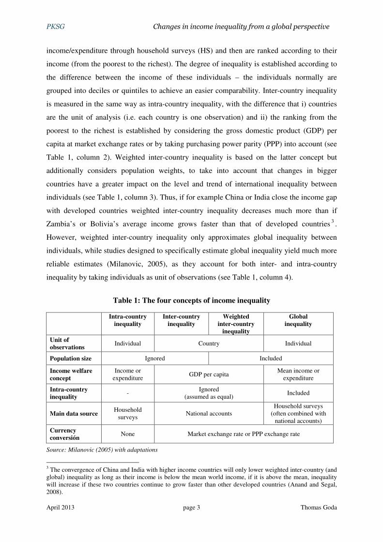
Table 1: The four concepts of income inequality

Intra-country

inequality

Inter-country

inequality

Weighted

inter-country

inequality

Global

inequality

Unit of

observations Individual Country Individual

Population size Ignored Included

Income welfare

concept

Income or expenditure

GDP per capita Mean income or

expenditure

Intra-country inequality

- Ignored

(assumed as equal) Included

Main data source Household

surveys National accounts

Household surveys (often combined with

national accounts)

Currency

conversión None Market exchange rate or PPP exchange rate

Source: Milanovic (2005) with adaptations

3 The convergence of China and India with higher income countries will only lower weighted inter-country (and global) inequality as long as their income is below the mean world income, if it is above the mean, inequality will increase if these two countries continue to grow faster than other developed countries (Anand and Segal, 2008).



The existing unequalness of income can be measured by various disproportionality

functions (see Cowell (2000) for an overview and discussion of different inequality indices).

However, the following discussion will be restricted to the two most common indicators to

ensure the comparability between the different results. The most widely used relative

inequality indicator is the Gini Index; because this index can be nicely represented

graphically, via the Lorenz curve, and that the lower bound (0 = total equality) and the upper

bound (1 = total inequality) can easily be understood by the broader public (Milanovic, 2005).

A second commonly used indicator in international inequality studies is the entropy based

Theil Index. This index also has zero as lower bound but the logarithm of the sample size as

upper bound (Theil, 1967). The Theil and the Gini Index, are the only indices that “satisfy

[all of] the five most highly desired properties of an inequality indicator: (1) it is symmetrical;

(2) it is income scale-invariant; (3) it is invariant to absolute population levels; (4) it is

defined by upper and lower bounds; (5) it satisfies the Pigou-Dalton principle of transfers

(any redistribution from richer to poorer reduces the inequality measure, and vice versa).”

(Korzeniewicz and Moran 2009, p. 123). Furthermore, to our knowledge at least one of these

two indices is mentioned in all inequality studies. This review will therefore concentrate on

these two indices to ensure the comparability between the different results.

The two main distinctions between the Gini and the Theil Index are their sensitivity to

transfers and their decomposability. An income transfer around the middle of the distribution

has a greater effect on the Gini coefficient than an income transfer from the top part of the

distribution to the bottom, whereas the opposite is true for the Theil coefficient (Cowell, 2000;

Korzeniewicz and Moran, 2009). However, both indices are highly correlated, e.g. a study by

Dikhanov (1996) shows that with regard to intra-country inequality the coefficient of

determination (r2) is around 0.998-0.999. Both indices can be decomposed into intra-group

and inter-group inequality, but the advantage of the Theil Index over the Gini Index is that it

can be additively decomposed if the subgroups are overlapping. In other words, the

advantage of the Theil Index is that it can exactly establish to what degree global inequality

changed due to increases/decreases in intra-country and inter-country inequality.



3. Changes in inter-country income inequality

Existing studies that measure unweighted inter-country inequality show that between 1820

and 2000 income inequality between countries increased substantially, i.e. a ‘Great

Divergence’ took place during this period4. Pritchett (1997) reports that from 1870 to 1990

“the ratio of per capita incomes between the richest and the poorest countries increased by

roughly a factor of five” (p.3). In 1870 the GDP per capita ratio between the richest and the

poorest country was 9. In 1960 this ratio was 39, and in 1990 the mean GDP per capita in the

richest country was 45 times higher than the mean GDP per capita of the poorest country.

The reason for this divergence is that during this period the vast majority of developing

countries had lower growth rates than high income OECD countries (i.e. Japan and the West

European countries and their offshoots: Australia, Canada, New Zealand, and the US).

Between 1960 and 1990, for example, 16 out of 108 developing countries had a negative

average growth rate, 28 had an average growth rate of less than 0.5, and 40 had an average

growth rate of less than one percent. Consequently, in 1990 the average GDP per capita of

high income OECD countries was 4.5 times higher than that of developing countries (in 1870

this ratio was 2.4).

The UNDP (1992) arrived at similar results and shows that the income ratio between the

richest 20% and the poorest 20% of countries increased twofold between 1960 and 1989 (in

PPP terms that ratio between the two groups was 50:1 in 1989) because the former countries

grew 2.7 times faster on average than the latter during this period. Firebaugh (1999) also

reports that inter-country inequality increased monotonously between 1960 and 1989. In a

more recent study, Milanovic (2005) shows that unweighted inter-country inequality already

started to increase after 1820 (with the exception of the period between World War I and

World War II): the Gini coefficient in 1820 was around 0.20 and increased to around 0.55 by

2000, i.e. it nearly tripled during these 180 years (see Figure 1a)5 . The reason for this

development was that some parts of the world, which initially had been relatively equal,

steadily diverged between 1870 and 2000 (while the mean incomes of rich OECD countries

were converging). The divergence in the post-1978 period apparently took place due to (i) the

sluggish growth performance in Latin America (following the debt crisis and the neoliberal

reforms), (ii) the decline in Eastern European/former Soviet Union incomes (following the

4 All of the discussed results are based on GDP per capita adjusted for purchasing power parity (PPP) exchange rates, as this measure is commonly used for the estimation of international inequality. 5 The increase between 1938 and 1960 can be partly explained by a greater country coverage (before 1938 less than 50 countries were included in the sample, after 1960 more than 125 countries were covered), however if the sample size is held constant the Gini still increases by 8 points.



collapse of the Eastern Bloc and the subsequent free market reforms), and (iii) the disastrous

economic developments within many African economies6.

Figure 1: Inter-country income inequality, 1820 - 2000

a. Unweighted

b. Weighted

Source: Milanovic (2005)

Weighted inter-country inequality, in contrast, shows a decreasing trend since the middle

of the 20th century (see Figure 1b). Similar to unweighted inter-country inequality Milanovic

(2005) gives the most comprehensive overview about historical changes. According to his

research, weighted inter-country inequality increased massively in the periods 1820 – 1929

and 1938 – 1952. The main reason for the distinct increase after 1938 can be attributed to

6 It is also interesting to note that between 1960 and 2000 the movement of countries “among contenders [i.e. upper middle-income countries] and the Third World was largely downwards. … [O]nly two countries (Botswana and Egypt) escaped from the trap of the Fourth World”, while 19 new countries entered this category in this period (Milanovic, 2005, p.68-70).



relative high growth figures of populous rich countries while populous poor countries were

growing relatively slowly in contrast to richer countries7. In turn, the main reason for the

decline in weighted inter-country income inequality after its peak in 1952 was “the

decreasing income gaps between the three most important countries (China, India, and the

United States)”. In the post-1978 period the main driver of this development was the fast

growth of China, i.e. if China were to be excluded from the sample the measured weighted

inter-country inequality would even increase slightly between 1978 and 2000.

Other researchers confirm Milanovic’s general findings, although they report that the

turning point was later. Schultz (1998, p. 328) reports that the “Gini concentration ratio based

on [weighted] inter-country PPP incomes increased about 6% from 1960 to 1968 and

thereafter decreased about 6% by 1985”. In the later years of his sample (i.e. between 1985

and 1989) the ratio increased slightly from 0.54 to 0.55, but the Gini coefficient in 1989 was

still significantly lower than it was in 1968 (0.58). According to Schultz’s research a change

in the world’s population composition was no major factor behind this decline in inequality.

Instead, the rapid growth rates of China, due to its huge population size, were the main factor

leading to the change in the trend of weighted inter-country inequality: in the 1960s China’s

growth was relatively low, while it was above the world’s average growth rate from the

1970s onwards. The findings from Boltho and Toniolo (1999) confirm and extend these

results: while the weighted inter-country Gini coefficient increased between 1960 (0.52) and

1970. It decreased thereafter from 0.54 in 1970 to 0.50 in 1998; mainly due to the “rapid

growth rates of India and, especially, China” (p. 6). Firebaugh (2003) also reports that

weighted inter-country inequality reached its maximum between 1965 and 1970 and

thereafter declined8.

Recent publications by Milanovic (2009, 2010b, 2012) suggest that the levels of inter-

country income inequality are even higher than originally expected (see Figure 2). The reason

for the higher pre-2000 inequality levels being new PPP data from the 2005 survey of the

International Comparison Program (ICP) because these new estimates led to a downward

revision of PPP GDP figures in 10 of the 13 most populous countries. As most of these

7 Some of the increase between 1938 and 1952 might be explained by the increasing sample size. However, the population coverage was already around 80% before 1952 as the most populous countries were included in the sample from 1820. Thus, the change in the sample size contributed only slightly to the increase in inequality (Milanovic, 2005). 8 Different studies report different inter-country Gini coefficients as they have (i) a different sample, (ii) different data sources, and/or (iii) different PPP estimates. These differences are not discussed in detail as the main results are very similar.



populous countries are relatively poor (e.g. in China, India and the Philippines PPP GDP

figures are around 40% lower than previously estimated9) income inequality is much higher

than previously thought, i.e. prior to 2000 inter-country inequality was around 5 and 8 Gini

points higher (compare Figure 1 with Figure 2). However, the revision has no trend effect

because the pre-2005 PPP GDP is estimated according to national GDP growth rates, and the

new PPP estimates have no impact on GDP growth rates (Milanovic, 2009).

Figure 2: Inter-country income inequality, 1952 - 2007

Source: Milanovic (2010b)

These new estimates from Milanovic also show that the ‘Great Divergence’ between

countries stopped and instead a convergence took place from 2000 onwards. The reasons for

this U-turn are the favorable economic developments in “African countries that have grown

at the rate of more than 4 percent per annum, post- Communist countries (growth at more

than 6 percent per annum), and Latin America (3 percent p.a.).” (ibid., 2012, pp.10).

However, although unweighted inter-country inequality was declining substantially after

2000, it was still much higher than prior to the 1990s. The reason is that, if taken as a group,

only the developing countries from East Asia and Pacific, and South Asia had a cumulative

average GDP per capita growth that was higher than the cumulative average GDP per capita

growth rate of high-income countries since 1971 (see Figure 3), i.e. only these two regions

could catch up with high income countries in the period 1971 to 2007.

9 Prior to the ICP 2005 survey the PPP estimates of India relied on 1985 survey estimates, and the ones of China were based on the results of two research papers as China never took part in any PPP survey prior to 2005 (Milanovic, 2009).

weighted

unweighted



Figure 3: Cumulative growth in GDP per capita relative to the world average

Note: The plot shows the cumulative difference between the world’s average per capita GDP growth and the

growth rates of high-income countries and of developing countries according to their region (Source: WDI

(2011); own calculations).

With regard to weighted inter-country inequality the downward trend in inequality

accelerated after 2000. The result was that weighted inter-country inequality decreased

roughly by 10 Gini points between 1960 and 2007 (see Figure 2). The acceleration mainly

took place because of stable high growth rates in China and rising growths rates in India. This

meant that not only China but also India put significant downward pressure on weighted

inter-country income inequality after 2000. Weighted inter-country inequality would thus

have also declined after 2000 if China would have been excluded from the sample. However,

despite these favorable developments inter-country inequality in 2007 was still much higher

than the inequality levels one normally finds within countries (see Section 5).

4. Changes in global income inequality

All studies that measure global income inequality have to choose between different

methodological options and different sources for their data. Depending on their choice their

estimated inequality will be higher or lower and the estimated trend may be different. In this

section therefore first some general methodological and data issues are discussed, then the

-60

-40

-20

0

20

40

60

80

100

120

140

160

Cu

mu

lati

ve

Dif

fere

nti

al

Gro

wth

High income East Asia & Pacific

Europe & Central Asia Latin America & Caribbean

Middle East & North Africa Sub-Saharan Africa

South Asia



methodology and data that are used by recent studies are analyzed, before finally the results

of these studies are summarized.

4.1. General methodological and data issues

While the choice between PPP and market exchange rates, and between different methods

to calculate PPP exchange rates also applies to studies that measure inter-country inequality

(see Table 1), only global inequality studies need to decide in favor of HS means or national

account means, expenditure or (gross or net) income, grouped or individual-level data, and

equivalent adult or per capita income (see Table 2). Next to the level, these choices can also

influence the trend in inequality (e.g. income inequality might increase while consumption

inequality might decrease at the same time due to increasing social transfers or higher saving

rates by the rich). Unfortunately, all of the data which is needed to calculate global inequality

have serious shortcomings and depending on the chosen indicators these problems might be

exacerbated, as will be discussed below.

Table 2: Possible indicators and their impact on the results

Possible Indicators

Indicator that leads

to lower inequality

estimates

Reason

PPP exchange rates vs. market exchange rates

PPP Poor countries have lower price levels ($1 buys more in Zimbabwe than in Germany)

GK PPP vs. Afriat or EKS PPP

GK PPP Poor countries’ incomes are overestimated (international prices are more influenced by rich countries – Gerschenkron effect)

GDP per capita vs. HS means or HFCE

HS means or HFCE Public expenditures are excluded (these are larger in rich countries)

Expenditure vs. (gross or net) income

Expenditure Expenditure tends to be more equally distributed (rich save substantial parts of their income)

Grouped data vs. individual-level data

Grouped data Income/expenditure differences between the individuals within quantiles are not considered

Equivalent adult vs. per capita

Equivalent adult Large households and households with many children do not require as many resources

To measure global inequality it is necessary to take into account intra-country inequality

coefficients for as many countries as possible. Typically, not the primary data from HS

compilations but datasets which report Gini coefficients and quantile shares are used for this

purpose. The best way to avoid inconsistency between the data of the latter is to use “data-



sets where the observations are as fully consistent as possible” (Atkinson and Brandolini,

2001, p.796). Unfortunately, even though more and more datasets with intra-country

inequality data compilation exist and the comparability and the quality of these data have

become better in recent years, none of these datasets provide data which are fully consistent.

The biggest problem is that national HS differ in their inequality concepts (consumption,

expenditure, net-income, or gross-income ), reference units (family, household, individual),

and sources (Francois and Rojas-Romagosa, 2007)10. A further problem is that most countries

only undertake HS every five years (or less often) and that the studies take place at different

points in time in different countries. Therefore, global inequality studies are forced to either

impute the missing values or to report only results for so called benchmark years (e.g. in

Milanovic’s (2005) study the benchmark year 1998 includes inequality coefficients of the

period 1996-2000). To my knowledge none of the existing datasets and global income studies

considers equivalent adult figures, as these are very hard to measure and also would differ

between countries (e.g. according to the costs for children’s goods and services).

So far, the two most widely used inequality datasets are the Deininger and Squire (DS)

database, which is available from the World Bank website, and the Word Income Inequality

Database (WIID) which is an extension of the DS dataset and administered by the United

Nations. The main problem with the DS dataset is that the estimates identified to be the most

reliable (labelled as ‘accept’) are related to different inequality concepts and mix different

reference units. DS therefore recommend to use dummy variables to deal with this problem

and to create a comparable series but as Atkinson and Brandolini (2001) have pointed out,

“simple ‘dummy variable’ adjustments for differences in definitions are not a satisfactory

approach” (p.795). WIID, in contrast, lists a wide range of Gini estimates, and quintile or

decile shares, which are based on different inequality concepts, reference units and/or sources.

However, this poses the problem that for many countries different inequality series exist and

that researchers have to identify which of these series are the most appropriate. Furthermore,

the problem persist that only quantile shares (quintiles or deciles) and not the individual data

are reported. Therefore, Milanovic has created two new datasets11: (i) the World Income

Distribution dataset (WYD), which is based on individual-level data whenever possible and

reports ventile shares and inequality coefficients for benchmark years, and (ii) the All The

Ginis dataset which takes into account distributional shares and Gini coefficients from the

10 Milanovic (2005) for example shows that between 1996-2000 59 out of 122 HS reported domestic income inequality while the remaining 63 reported domestic expenditure inequality. 11 These are relatively frequently updated and available on the World Bank website.



Luxembourg Income Studies (LIS), the Socio-Economic Database for Latin America and the

Caribbean (SEDLAC), the WYD, the World Bank East and Central Europe database (ECA),

and the WIID dataset. However, even with this improvement in the comparability two

problems persist. First, HS surveys are still based on different income concepts, and second,

the Ginis of the different sources are calculated from grouped and from individual-level data,

depending on the source (Milanovic, 2010a). Hence, at least, an adjustment for the different

income concepts is still needed to use the data of these dataset for empirical work.

The second problem with regard to the measurement of global inequality is that typically

PPP exchange rates are used when the Gini coefficients of countries are scaled to national

account means or household means. Three different methods have been used in recent years

to construct the domestic price levels: (i) the Geary-Khamis (GK) Method, (ii) the Eltetö-

Köves-Szulc (EKS) method, and (iii) Afriat’s method. Most authors argue that PPP exchange

rates are superior to market exchange rates because the latter do not reflect that domestic

goods and services in poor countries are much cheaper than in richer countries, and therefore

inequality would be overstated if market exchange rates would be used instead of the

domestic price level. However, relatively little discussion has taken place in inequality

studies regarding the shortcomings of the different methods and the PPP approach in general.

Most studies that have measured global inequality so far use GK PPP data12. Although the

GK method is inferior to the EKS method and Afriat’s method because it gives higher weight

to the prices of richer countries: rich countries have a higher share in world output. This

means that the international prices used in the GK method to construct the PPP exchange rate

for every country are closer to the price levels of richer countries. This leads to inflated PPP

figures for poor countries because this method does not sufficiently consider that expensive

products are substituted by cheaper ones in poorer countries – this problem is called

substitution or Gerschenkron bias (ibid, 2005; Anand and Segal, 2008). The EKS method and

Afriat’s method do not suffer from this bias (as they do not construct a vector of international

prices) and are therefore preferable when estimating PPP exchange rates. Unfortunately, the

Afriat Index cannot be calculated for all countries as it requires that countries have ‘common

homothetic preferences’. Therefore, the most appropriate indicator for global inequality

studies would be PPP exchange rates which are constructed via the EKS method (Anand and

Segal, 2008). Fortunately, the newest ICP study from 2005 uses the EKS method to estimate

PPP exchange rates. However, even when this method is used three general problems persist:

12 The GK method was used to construct the Penn World Tables and by Maddison for his datasets.



ICP PPP studies are only undertaken every five years, and not all countries are directly

included in this study, so that the results are based on a representative basket of goods and

services which can differ from country to country (for an extensive analysis of the problems

associated with PPP data see Deaton (2010)).

Even if most of the aforementioned measurement problems were to be solved (e.g. via a

global HS which take place every year, and yearly PPP measurements which include all

countries), the problem of survey sampling error, non-response, underreporting, and

misreporting, and top-coding still prevails. With sampling error it is meant that very poor (as

they often have no registered address) and very rich households (as they are not easily

accessible) often are underrepresented in the sample. Underreporting of income and

nonresponse is mainly a problem with regard to rich households (e.g. due to top-coding). The

same possibly is true for misreporting, e.g. for investment and property income, although

individuals throughout the distributional ladder, like micro-enterprises, often are unsure about

their actual income and/or expenditure (for more detailed information on these topics see

Atkinson and Brandolini, 2001; Deaton, 2005; Milanovic, 2005; Anand and Segal, 2008;

Pinkovskiy and Sala-i-Martin, 2009). In addition, “many income surveys are ‘top coded’ –

that is incomes above a certain threshold are lumped together [so that they] fail to capture the

potentially huge distribution … within that top code” (Shaxson et al., 2012, pp.13). The

outcome of these survey problems means that intra-country income inequality is

underestimated, thereby leading to an underestimation of global inequality13.

Most studies that try to measure global income inequality use GDP per capita and not HS

means for the reason that GDP per capita is readily available for most countries on an annual

basis for a long-time period, whereas HS only started to become available since the 1980s.

Furthermore, it is claimed (see e.g. Bhalla, 2002) that HS means underestimate income and

therefore GDP per capita is a better indicator to be used. However, next to the point that it is

strange to assume that HS results can be used to establish intra-country inequality but not the

average income levels of the country (Milanovic, 2005), two very important points speak

against the usage of GDP per capita. Firstly, GDP entails retained earnings, depreciation and

non-redistributed government revenue; thus, personal income/expenditure is overestimated

when GDP per capita is used (Anand and Segal, 2008). This upscaling of income/earnings

13 For this reason Milanovic (2010b) claims that it would be better to measure consumption inequality as “consumption surveys are more reliable because the underestimate of consumption by the rich is less than the underestimate of income by the rich.” (p.11)



not only changes the level but also can have an impact on the trend, if GDP per capita and HS

means are not changing proportionally, which often is the case. Secondly, although GDP per

capita entails the unreported and misreported income of the rich, it does not solve but rather

exacerbates the underestimation problem because the incomes of all quantiles are upscaled by

the same proportion (i.e. if GDP per capita is 20% higher than the HS mean, the income of all

quantiles is upscaled by 20%).

Another national account figure which also is readily available for most countries is

household final consumption expenditure (HFCE). However, although this indicator seems to

be a much better proxy of income/expenditure than GDP – according to Deaton (2005) the

population weighted mean ratio of HS income means to GDP is 0.54 (272 surveys) while the

ratio is 1 with regard to HFCE (266 surveys) – it also has certain drawbacks. Firstly, it

includes expenditure from nonprofit organizations and imputed rents. Secondly, HFCE is a

residual value (national production minus government and firm’s consumption) whose

amount is influenced by possible errors in estimating national production and government

and firm’s consumption; especially the first and the latter are often only rough estimates

(Anand and Segal, 2008). Consequently, HS means seem to be the first best indicator when

measuring global inequality, while the ‘upscaling’ via HFCE or GDP per capita is only the

second and least best option respectively.

4.2. Methodology and data used by studies

Table 3 gives an overview about the main methods applied by studies published between

2005 and 2011 – Bourguignon and Morrison’s (2002) study is included as only two recent

studies researched long-term global inequality trends. In general it can be said that the study

from Milanovic (2012) is the sole study that has used the ‘best available indicators’ (i.e. EKS

PPP exchange rates, HS means, and individual-level data wherever this is possible) to

estimate global income inequality. Furthermore, it becomes visible that some studies are

using approximation techniques for missing years and mix households and individuals as unit

of analysis (as discussed above the DS dataset mixes the two); both can distort the results

significantly.

PKSG

Changes in

income inequality from a global perspectiv

e

Ap

ril 20

13

pag

e 15

Tho

mas G

od

a

Tab

le 3: R

ecent g

lob

al in

equ

ality

stud

ies an

d th

eir meth

od

s an

d d

ata

Coverage Income meanPPP

exchange rateHS data source

Expenditure

/incomeunit of analysis

grouped / individual

level data

approximation of missing

distributional data

Bourguignon &

Morrison (2002)

15 countries and 18

country groups

1820 - 1992

GDP per capita

(Maddison 1995)GK various mixed not clear

nine deciles and two

vintiles (of the top)

yes

(similar countries)

Chotikapanich et al. (2009)91 countries

1993 and 2000

GDP per capita

(PWT 6.1)GK WYD and WIID mixed households

beta-2 approx. of

distribution from quantile

data

no

Dikhanov (2005)45 countries

1970 - 2000

HFCE

(World Bank data)EKS not clear mixed not clear

quasi-exact polynomial

interpolation of distributionnot clear but most likely

Dowrick & Akmal (2005)67 countries

1980 and 1993

GDP per capita

(own estimates)Afriat DS mixed

mix of individuals

& households

quintiles

(parametric approx. if only

Gini coef. available)

no

Holzmann et al. (2010)114 countries

1970 - 2003

GDP per capita

(PWT 6.2)GK

WIID

(adjusted by Grün

& Klasen, 2007)

mixed households

parametric (log-normal)

approx. of distribution from

quintile data

yes

(not exactly clear how)

Milanovic (2005)

122

(86 common sample)

1988, 1993, 1998

HS mean GK

mainly micro data

(some grouped data

from World Bank)

mixed individuals

ventiles

(sometimes deciles or

quintiles)

no

Milanovic (2012)124

1988 - 2005HS mean EKS

mainly micro data

(some grouped data

from World Bank)

mixed individuals

ventiles

(sometimes deciles or

quintiles)

no

Pinkovskiy &

Sala-i-Martin (2009)

191 countries

1970 - 2006

GDP per capita

(PWT 6.2 and

own extension)

GK

WIID and

POVCAL for

China and India

mixedmix of individuals

& households



quintile data

yes

(linear trend or same

distribution in all years)

Sala-i-Martin (2006)138 countries

1970 - 2000

GDP per capita

(PWT 6.1)GK DS and WIID mixed

mix of individuals

& households

Kernel estimation of

distribution from quintile

data

yes

(linear trend or same

distribution in all years)

Van Zanden et al. (2011)

39 - 99 countries

(core group 30 countries)

1820 - 2000

GDP per capita

(Worldbank 2008,

growth rates from

Maddison 2003)

EKS various mixed not clear



Gini coefficients

yes

(top income shares, unskilled

wages, population heights,

and interpolation)



To be more precise, Bourguignon and Morrison (2002) estimate global income inequality

in 15 benchmark years between 1820 and 1992 by gathering data for eighteen groups of

countries (e.g. a group of 46 African countries, 37 Latin American countries, Argentina and

Chile, Scandinavia) and 15 populous individual countries (e.g. China, Brazil, Germany, India,

US). They combine the income shares of the bottom nine deciles and top two ventiles

(assuming equal distribution within these quintiles) with historical GPD per capita data from

Maddison (which they needed to extend for some countries) for their estimates. In years

where distribution data was missing for groups/countries the distribution was assumed to be

the same as in similar groups/countries; in the case of missing GDP data the Maddison series

was extended by using growth rates of neighboring countries.

This approach was extended in a recent publication from van Zanden et al. (2011). The

main changes are the extension of the distribution dataset and the incorporation of the new

ICP 2005 PPP estimates (using the growth rates from Maddison). First, van Zanden et al.

generated a new Gini coefficient dataset by (i) using WIID data, (ii) incorporating inequality

estimates of historical studies ‘overlooked’ by Bourguignon and Morrison, (iii) estimating the

distribution according to income shares of the top 1% and 5% (assuming log-normality), (iv)

using proxies to calculate Gini coefficient, namely the ratio between GDP per capita and real

wages of unskilled workers and the distribution of heights within the population of a country,

and (v) using some interpolation to be able to get estimates in all years for a core-group of 30

countries. From the resulting data the income distributions of all countries is calculated by

assuming that their intra-country distribution is log-normal. This distributional data is then

scaled to the calculated GDP per capita estimates. Interestingly, the resulting level and trend

of global inequality is very similar to Bourguignon and Morrison’s results (see Figure 7 in the

next section).

Milanovic (2005) argues that the usage of approximations, country groups, and GDP per

capita data is suitable if historical trends are studied but that this approach is not justifiable

anymore if actual HS data is available. Therefore, he constructs the WYD dataset with a

common sample of 86 countries (in total the dataset has data from 122 countries) for the

benchmark years 1988, 1993 and 1998 , relying mainly on micro data from HS and to some

extent on grouped data from World Bank sources. From the micro data he forms ventiles and

uses decile or quintile data, according to availability, for the countries for which only grouped

data is accessible. Milanovic, like Bourguignon and Morrisson, assumes that the income

within these quantiles is equally distributed. In contrast to the other studies, he uses HS



means (adjusted by GK PPP) to scale these income distributions to be able to estimate global

income inequality. Milanovic (2012) updates the estimates for the years 2002 and 2005 using

the same approach but the new ICP 2005 PPP estimates are based on the EKS method.

According to Anand and Segal (2008), Milanovic’s approach has two major weaknesses.

Firstly, his assumption that the distribution within quintiles is constant leads to an

underestimation of inequality, especially due to populous countries like China and India .

Secondly, the amount of quantiles per country is not constant over time (e.g. for the 1993

benchmark more micro data is available than for the 1988 benchmark) which leads to

changes in the underestimation of inequality. As a response to the first criticism, Milanovic

(2012) shows that the underestimation accruing from the usage of ventile data is minimal: by

comparing Gini coefficients calculated from micro data and from ventile data he shows that

the underestimation is around 1%.

Dowrick and Akmal (2005) also use benchmark years (1980 and 1993) and assume equal

distribution within quantiles, but in contrast to Milanovic (2005, 2012) they use Afriat PPP

exchange rates to measure global income distribution. The main problems with their

approach, next to the assumption of equal distribution, is that they are using data from the DS

dataset which mixes individuals and households and that they scale the distribution with GDP

per capita. To circumvent the underestimation of inequality Chotikapanich et al. (2009)

calculate continuous beta-2 household income distributions for 91 countries from the quantile

data of the WYD and WIID dataset. However, the weakness of their study is that these beta-2

income distributions are combined with GDP per capita data and not with HS means . Only

one recent study that uses benchmark years scales distributional data with HFCE to estimates

global income inequality. Unfortunately, it does not become clear from Dikhanov’s (2005)

paper which data (source) he uses to estimate his quasi-exact polynomial distribution data

which he scales by HFCE but it is likely that the data for some countries is approximated,

given that the distributional data that are used are not readily available for all of the 45

countries for all benchmark years (i.e. 1970, 1980, 1990, and 2000).

Sala-i-Martin (2006) was the first person to estimates the global income distribution for all

years of the period 1970 to 2000. To be able to achieve this, and to be able to take into

account 137 countries, Sala-i-Martin did not distinguish between households and individuals

and more importantly he needed to approximate most of his distributional data – only for one

country, the US, annual distributional data is available for the whole period. To be more

precise, for the 80 countries for which several observations are available from the DS and



WIID dataset he uses a linear trend to fill the gaps (his so called group A countries), for the

29 countries for which only one HS survey result exists he imputes the missing years by

using the average trend of the region to which the country belongs (group B countries), and

for the 28 countries for which no HS data exists he approximates the distribution for all years

according to the average quintile share and trend of neighbouring countries (group C

countries). After having approximated the majority of the distributional data, he estimates a

continuous distribution by using a nonparametric kernel density function. This income

distribution is scaled with PPP GPD per capita estimates from the Penn World Tables.

Sala-i-Martin’s approach has been heavily criticized by Milanovic (2002) and Anand and

Segal (2008). The first critique was that the distribution had been estimated from very few

data points (i.e. quintiles) which are derived “from grouped data and estimated by fitting the

Lorenz curves. Thus, quintiles which are themselves estimates are used to estimate the entire

distributions.” (Milanovic, 2002, p.10). This criticism is also valid for the studies of

Chotikapanich and Dikhanov. However, Sala-i-Martin uses a kernel density estimation which

should only be used when many independently and identically distributed data points are

available and – beside the point that only few data points are available – these “quintile

means used by Sala i-Martin are ‘trimmed means’ … based on ordered income data and are,

therefore, neither independently nor identically distributed” (Anand and Segal, 2008, p.78).

To make matters worse, Sala-i-Martin uses a constant bandwidth for all countries and years

which is erroneous. In a nutshell, his nonparametric estimates seem not very reliable. The

second critique is “the sparseness of the data which is an even more serious problem.”

(Milanovic, 2002, p.14). The income distribution of countries can vary significantly from HS

to HS without having a linear trend and the inequality levels and trends of countries within a

region often differ significantly. Therefore, Sala-i-Martin’s approach is a “dramatic

oversimplification with an unknown bias.” (ibid, p.16).

To overcome the critique regarding the non-parametric estimation, Pinkovskiy and Sala-i-

Martin (2009) have measured the income distribution by using a lognormal functional form.

As Sala-i-Martin (2006) they use quintiles and scale the distribution to GDP per capita means

(to be able to estimate the whole period with PWT 6.2 GDP per capita estimates they are

extending the PWT data for the years 2005 and 2006, assuming that the GDP per capita

growth rate in these years corresponds to a 4-year moving average). Nevertheless, Pinkovskiy

and Sala-i-Martin approximate even more distributional data than Sala-i-Martin as they are

including 191 countries (plus rural China and India) in their estimates. This means that for



about half of all countries only one or none HS result exists, on average only 5.5 surveys per

country are available for this 36 year period, and on average only 25% of the world

population is covered directly every year. Pinkovskiy and Sala-i-Martin try to improve Sala-i-

Martin’s approximations by testing different interpolation (missing years between known

distributions) and extrapolation (missing years before the first and last known distribution)

methods. However, with regard to the latter it becomes necessary to down weight within

country Gini coefficients if a trend is assumed as some “extrapolations violate the range of

the Gini in the survey data (from 0.17 to 0.81)” (p.14). This problem confirms Milanovic’s

(2002) critique about the unreliability of estimated distributional data. Therefore, Pinkovskiy

and Sala-i-Martin choose to extrapolate distributional data by horizontal projection (i.e. the

Gini coefficient is assumed to remain constant), while interpolation between known

distribution takes place by using piecewise cubic splines.

Holzmann et al. (2007) also use a lognormal functional form and are scaling distributional

data with GDP per capita to try to improve Sala-i-Martin’s (2006) estimates and they have

less heroic approximations than Pinkovskiy and Sala-i-Martin (2009) with regard to country

and year coverage. However, they too have needed to use massive approximations to be able

to cover the distribution of 114 countries in 5 year intervals between 1970 and 2000 and for

2003. They firstly assumed that the level of inequality in 1970 was the same as at first

reported level of inequality (i.e. horizontal projection), and secondly they used a “moving

average to catch changes in trends of inequality.” (p.5). Hence, both, Pinkovskiy’s and Sala-i-

Martin’s, and Holzmann et al.’s study have an unknown bias.

4.3. Results of existing global inequality studies

The two most prominent researchers with regard to global income inequality are arguably

Milanovic and Sala-i-Martin. When one has a look at their two latest estimates (stand

October 2012) in Figure 4, it becomes immediately visible that global income inequality

estimates (i.e. the trend and the level) differ significantly depending on the methods and data

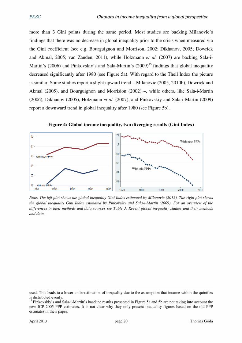
used. While Milanovic (2012) reports that the global Gini coefficient increased by around 2

points between 1988 and 2005 when the new ICP 2005 PPP estimates are taken into

account14, Pinkovskiy and Sala-i-Martin (2009) claim that the Gini coefficient decreased by

14 The increase might be due to an increase of available micro data over time. In 1988 for 45 out of 103 countries micro data is available while in 2002 and 2005 for 117 out of 122 countries micro data is available). This change in the availability of micro data means that over time more ventile and less decile or quantile data is



more than 3 Gini points during the same period. Most studies are backing Milanovic’s

findings that there was no decrease in global inequality prior to the crisis when measured via

the Gini coefficient (see e.g. Bourguignon and Morrison, 2002; Dikhanov, 2005; Dowrick

and Akmal, 2005; van Zanden, 2011), while Holzmann et al. (2007) are backing Sala-i-

Martin’s (2006) and Pinkovskiy’s and Sala-Martin’s (2009)15 findings that global inequality

decreased significantly after 1980 (see Figure 5a). With regard to the Theil Index the picture

is similar. Some studies report a slight upward trend – Milanovic (2005, 2010b), Dowrick and

Akmal (2005), and Bourguignon and Morrision (2002) –, while others, like Sala-i-Martin

(2006), Dikhanov (2005), Holzmann et al. (2007), and Pinkovskiy and Sala-i-Martin (2009)

report a downward trend in global inequality after 1980 (see Figure 5b).

Figure 4: Global income inequality, two diverging results (Gini Index)

Note: The left plot shows the global inequality Gini Index estimated by Milanovic (2012). The right plot shows

the global inequality Gini Index estimated by Pinkovskiy and Sala-i-Martin (2009). For an overview of the

differences in their methods and data sources see Table 3: Recent global inequality studies and their methods

and data.

used. This leads to a lower underestimation of inequality due to the assumption that income within the quintiles is distributed evenly. 15 Pinkovskiy’s and Sala-i-Martin’s baseline results presented in Figure 5a and 5b are not taking into account the new ICP 2005 PPP estimates. It is not clear why they only present inequality figures based on the old PPP estimates in their paper.

With new PPPs

With old PPPs



Figure 5: Various pathways of global income inequality since the 1970s

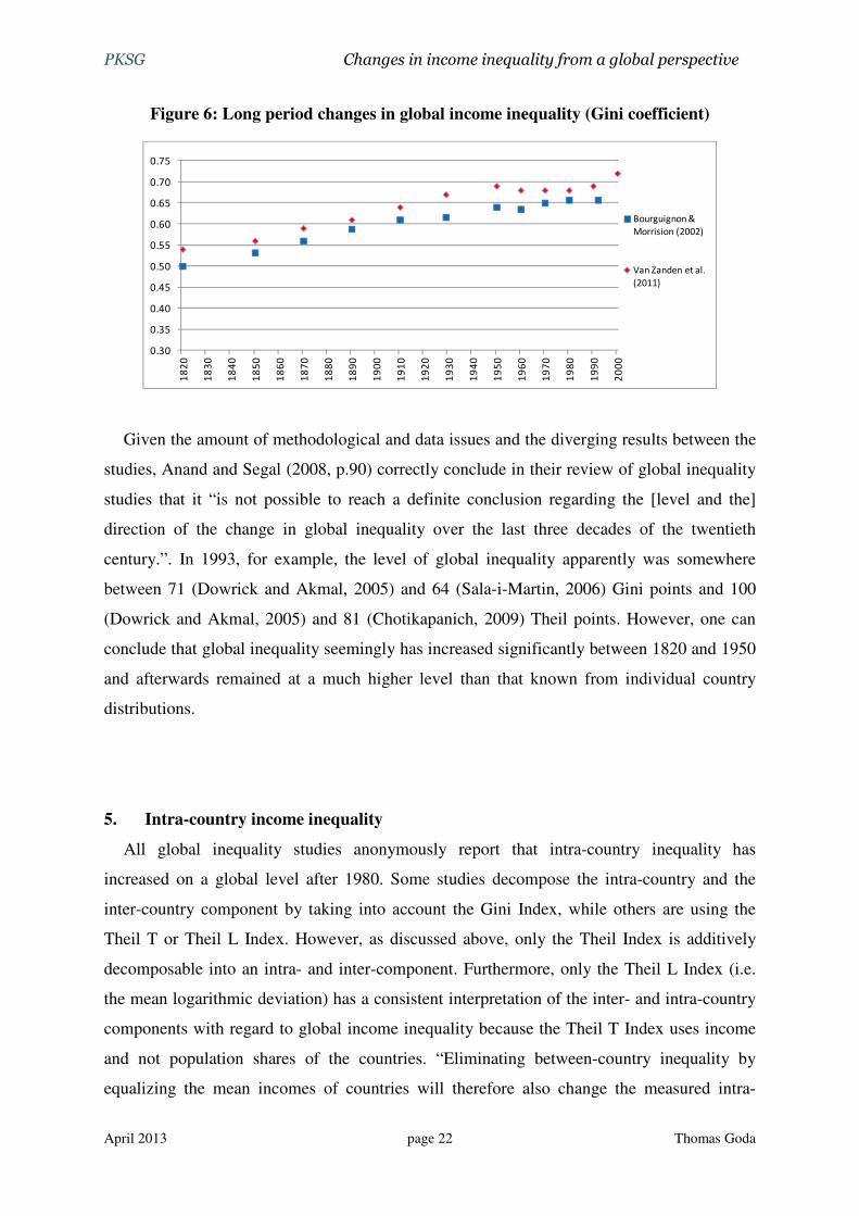
With regard to historical changes the picture seems to be much clearer. The two existing

studies that researched the level and trend of global inequality since 1820, Bourguignon and

Morrison (2002) and van Zanden et al. (2011), reported that global inequality levels were

much lower in the 19th century and at the beginning of the 20th century than in the late 20th

century. To be more precise, between 1820 and 1950 global income inequality increased

steadily, in total by around 15 Gini points, while it leveled off afterwards (see Figure 6). The

main reason why van Zanden et al.’s estimated level of inequality is persistently higher than

that estimated by Bourguignon and Morrison is that the former are using the new ICP 2005

PPP estimates in their analysis.



Figure 6: Long period changes in global income inequality (Gini coefficient)

Given the amount of methodological and data issues and the diverging results between the

studies, Anand and Segal (2008, p.90) correctly conclude in their review of global inequality

studies that it “is not possible to reach a definite conclusion regarding the [level and the]

direction of the change in global inequality over the last three decades of the twentieth

century.”. In 1993, for example, the level of global inequality apparently was somewhere

between 71 (Dowrick and Akmal, 2005) and 64 (Sala-i-Martin, 2006) Gini points and 100

(Dowrick and Akmal, 2005) and 81 (Chotikapanich, 2009) Theil points. However, one can

conclude that global inequality seemingly has increased significantly between 1820 and 1950

and afterwards remained at a much higher level than that known from individual country

distributions.

5. Intra-country income inequality

All global inequality studies anonymously report that intra-country inequality has

increased on a global level after 1980. Some studies decompose the intra-country and the

inter-country component by taking into account the Gini Index, while others are using the

Theil T or Theil L Index. However, as discussed above, only the Theil Index is additively

decomposable into an intra- and inter-component. Furthermore, only the Theil L Index (i.e.

the mean logarithmic deviation) has a consistent interpretation of the inter- and intra-country

components with regard to global income inequality because the Theil T Index uses income

and not population shares of the countries. “Eliminating between-country inequality by

equalizing the mean incomes of countries will therefore also change the measured intra-

0.30

0.35

0.40

0.45

0.50

0.55

0.60

0.65

0.70

0.75

18

20

18

30

18

40

18

50

18

60

18

70

18

80

18

90

19

00

19

10

19

20

19

30

19

40

19

50

19

60

19

70

19

80

19

90

20

00

Bourguignon &

Morrision (2002)

Van Zanden et al.

(2011)



country component: the elimination will leave a population-weighted average of the Theil T

indices of countries, not the original income-weighted average.” (Anand and Segal, 2008,

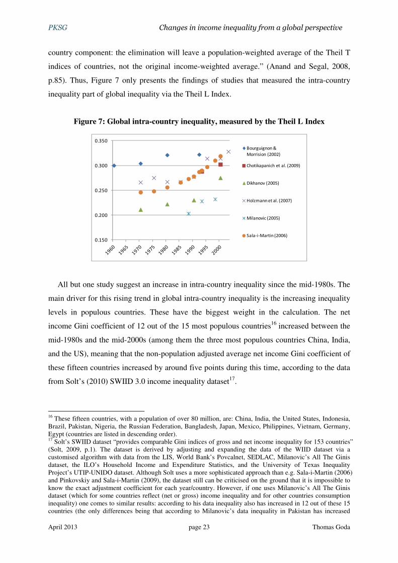
p.85). Thus, Figure 7 only presents the findings of studies that measured the intra-country

inequality part of global inequality via the Theil L Index.

Figure 7: Global intra-country inequality, measured by the Theil L Index

All but one study suggest an increase in intra-country inequality since the mid-1980s. The

main driver for this rising trend in global intra-country inequality is the increasing inequality

levels in populous countries. These have the biggest weight in the calculation. The net

income Gini coefficient of 12 out of the 15 most populous countries16 increased between the

mid-1980s and the mid-2000s (among them the three most populous countries China, India,

and the US), meaning that the non-population adjusted average net income Gini coefficient of

these fifteen countries increased by around five points during this time, according to the data

from Solt’s (2010) SWIID 3.0 income inequality dataset17.

16 These fifteen countries, with a population of over 80 million, are: China, India, the United States, Indonesia, Brazil, Pakistan, Nigeria, the Russian Federation, Bangladesh, Japan, Mexico, Philippines, Vietnam, Germany, Egypt (countries are listed in descending order). 17 Solt’s SWIID dataset “provides comparable Gini indices of gross and net income inequality for 153 countries” (Solt, 2009, p.1). The dataset is derived by adjusting and expanding the data of the WIID dataset via a customised algorithm with data from the LIS, World Bank’s Povcalnet, SEDLAC, Milanovic’s All The Ginis dataset, the ILO’s Household Income and Expenditure Statistics, and the University of Texas Inequality Project’s UTIP-UNIDO dataset. Although Solt uses a more sophisticated approach than e.g. Sala-i-Martin (2006) and Pinkovskiy and Sala-i-Martin (2009), the dataset still can be criticised on the ground that it is impossible to know the exact adjustment coefficient for each year/country. However, if one uses Milanovic’s All The Ginis dataset (which for some countries reflect (net or gross) income inequality and for other countries consumption inequality) one comes to similar results: according to his data inequality also has increased in 12 out of these 15 countries (the only differences being that according to Milanovic’s data inequality in Pakistan has increased

0.150

0.200

0.250

0.300

0.350

Bourguignon &

Morrision (2002)

Chotikapanich et al. (2009)

Dikhanov (2005)

Holzmann et al. (2007)

Milanovic (2005)

Sala-i-Martin (2006)



If one looks at the individual Gini coefficients of countries, it becomes immediately

apparent that since the mid-1980s intra-country income inequality has increased in most high

income countries and in most developing European and Asian countries prior to the crisis18

(see Figure 8a-c), while it was on average relatively stable in Latin American and the

Caribbean, and Middle Eastern and North African developing countries, and declining in

Sub-Saharan Africa (see Figure 8d-e). However, intra-country income inequality levels were

still much lower than the level of global income inequality19, i.e. the population unadjusted

average inequality was around 30 Gini points in high-income countries, 35 Gini points in

European and Central Asian developing countries, 40 Gini points in East and South Asian

and in Middle Eastern and North African developing countries, 45 Gini points in Sub-

Saharan countries, and 50 Gini points in Latin American and Caribbean developing countries

for which data is available.

The changes in inequality and its levels suggest that Li et al.´s (1998) and Korzeniewicz

and Moran’s (2009) finding that intra-income inequality is relatively stable over time.

Countries can be clustered into a high-inequality and a low-inequality group is questionable –

because according to the former inequality depends on civil liberties, the level of secondary

schooling, financial depth and the initial distribution of land, while the latter claim that one

group consists of Western countries and their offshoots that had and have ‘good’ institutions

and a low inequality equilibrium (below 33 Gini points), while the high inequality

equilibrium group (above 50 Gini points) consists of ‘ex-plantation colonies’ where elites

were and are dominant while huge parts of the population were and are subordinated.

Moreover, this data does not support Kuznets’ (1955, 1965) hypothesis that during the path of

development inequality should first rise, as more people are getting employed in the non-

agricultural sector which pays higher wages on average, and then steadily fall when an

increasing majority of people are employed in the high-income sector, i.e. when the

proportion of middle-income earners increases and the proportion of poor subsistence farmers

decreases. According to Kuznets´ analysis the intra-country inequality thus should have an

inverted-U shaped form and its level should be clearly related to the economic development

of the country (i.e. to its GDP per capita).

while it has decreased in Nigeria), leading to an (non-population adjusted) average increase in the Gini coefficient by around four points. 18 In most countries the increase in inequality was most pronounced between the mid-1980s and the mid-1990s and in some countries inequality even declined slightly after the mid-1990s. 19 The only two countries which had pre-crisis inequality levels which were similar to the magnitude of global income inequality were South Africa and Namibia.



Figure 8 Change in intra-country income inequality (Gini coefficient)

Note: These plots show changes in net income inequality. For marked countries the initial value shows 1990 (or

close to that year) Gini coefficients. The pre-crisis values are Gini coefficients of the year 2007 or the latest

available figure after 2003 (data source: Solt (2010)).

However, this inverted-U shape is not observable empirically and therefore “changes in

inequality may be better described as ‘episodic’ rather than as long-run trends” (Atkinson,

1997, p.300). The changes in intra-income inequality prior to the crisis might therefore be

best explained by (i) wage dispersion and technological change, (ii) changes in the bargaining

power of workers, (iii) changes in social norms, (iv) demographic changes, (v) education

policies, (vi) returns on capital, (vii) inheritance and initial inequality differences, and (viii)

changes in the income distribution policies and taxation policies (ibid, 1979). This variety of

complex processes means that the typical worker vs. capitalist class identity is still important

but to some extent blurred (Franzini and Pianta, 2011).

15.0

20.0

25.0

30.0

35.0

40.0

45.0

50.0

55.0

60.0

65.0

70.0

Ho

ng

Ko

ng

Est

on

ia

Jap

an

Slo

ve

nia

Un

ite

d K

ing

do

m

Isra

el

Ne

w Z

ea

lan

d

Cze

ch

Re

pu

bli

c

Hu

ng

ary

Slo

va

k R

ep

ub

lic

Pu

ert

o R

ico

Po

rtu

ga

l

Fin

lan

d

Po

lan

d

Lu

xe

mb

ou

rg

Un

ite

d S

tate

s

Au

stri

a

Ta

iwa

n

Au

stra

lia

Av

era

ge

Sp

ain

Ca

na

da

Be

lgiu

m

Ge

rma

ny

Sw

ed

en

Ita

ly

Ne

the

rla

nd

s

No

rwa

y

Gre

ec

e

Sw

itze

rla

nd

De

nm

ark

Cro

ati

a

Fra

nc

e

Ire

lan

d

Tri

nid

ad

& T

ob

ag

o

Ko

rea

a. High-income countries

mid-1980s

pre-crisis

increasing little change decreasing

15.0

20.0

25.0

30.0

35.0

40.0

45.0

50.0

55.0

60.0

65.0

70.0

Ne

pa

l

Ch

ina

Sri

La

nk

a

Ba

ng

lad

esh

Ph

ilip

pin

es

Sin

ga

po

re

Av

era

ge

Ind

ia

Vie

tna

m*

Ind

on

esi

a

Pa

kis

tan

Ma

lay

sia

Th

ail

an

d

b. East Asian and South Asian developing countries

mid-1980s

pre-crisis

increasing decreasing

15.0

20.0

25.0

30.0

35.0

40.0

45.0

50.0

55.0

60.0

65.0

70.0

Ru

ssia

n F

ed

era

tio

n

Tu

rkm

en

ista

n

Ky

rgy

z R

ep

ub

lic

Arm

en

ia

Mo

ldo

va

Lit

hu

an

ia

Ge

org

ia

La

tvia

Uzb

ek

ista

n

Ro

ma

nia

*

Ka

zak

hst

an

Av

era

ge

Bu

lga

ria

Ma

ce

do

nia

*

Ta

jik

ista

n

Uk

rain

e

Be

laru

s

Se

rbia

Tu

rke

y

Bo

snia

& H

erz

og

.*

Aze

rba

ija

n

c. European and Central Asian developing countries

mid-1980s

pre-crisis

increasing decreasing

15.0

20.0

25.0

30.0

35.0

40.0

45.0

50.0

55.0

60.0

65.0

70.0

Pa

rag

ua

y*

Pe

ru

Co

sta

Ric

a

Ec

ua

do

r

Arg

en

tin

a

Co

lom

bia

Do

min

ica

n R

ep

.

Uru

gu

ay

Me

xic

o

Bo

liv

ia

Av

era

ge

Pa

na

ma

El

Sa

lva

do

r

Ho

nd

ura

s

Bra

zil

Ve

ne

zue

la

Ch

ile

Gu

ate

ma

la

Jam

aic

a

d. Latin American and Caribbean developing countries

mid-1980s

pre-crisis

increasing decreasinglittle change

15.0

20.0

25.0

30.0

35.0

40.0

45.0

50.0

55.0

60.0

65.0

70.0

Jord

an

Mo

roc

co

Av

era

ge

Ye

me

n*

Tu

nis

ia

Eg

yp

t

Alg

eri

a

Ira

n

e. Middle East earn and North African developing countries

mid-1980s

pre-crisis


15.0

20.0

25.0

30.0

35.0

40.0

45.0

50.0

55.0

60.0

65.0

70.0

Ca

pe

Ve

rde

*

So

uth

Afr

ica

Ma

uri

tiu

s*

Gh

an

a

Nig

er*

Ma

li*

Nig

eri

a

Ug

an

da

Ma

da

ga

sca

r

Bo

tsw

an

a

Za

mb

ia

Na

mib

ia*

Av

era

ge

Eth

iop

ia

Ke

ny

a

Gu

ine

a*

Ga

bo

n*

Le

soth

o

Gu

ine

a-B

issa

u*

Sie

rra

Le

on

e

Ma

law

i

Se

ne

ga

l*

f. Sub-Saharan African developing countries

mid-1980s

pre-crisis




According to recent empirical results the most important reason for the increasing income

inequality in OECD countries was that in most of these countries the household income of the

top decile was growing faster than that of the bottom decile and the total population (OECD,

2011). This gives support to Palma’s (2011) hypothesis that the share of the rich is the most

important determinant for the level of intra-country inequality. This increase in top incomes

can be mainly explained by (i) an under-proportional increase of real wages compared to

productivity which means that the (adjusted) profit share since 1980 rose by “some ten

percentage points in continental European countries, and even more in Japan [and by] around

five percentage points” in the UK and US (Stockhammer, 2012a, p.8) 20 ; (ii) the over-

proportional increase of top management and superstar wages (especially in Anglo-Saxon

countries) – while at the same time workers at the bottom often witnessed declining real

wages (see e.g. Ellis and Smith (2010), ILO (2008), Atkinson et al. (2011) and Hein (2011);

and (iii) the more unevenly distributed capital income (see e.g. OECD (2011)).

The resulting increase in market income inequality was not offset by redistributive policies

because market income inequality was growing twice as fast as redistributive transfers, partly

for the reason that redistributive policies in rich countries became weaker in the decade prior

to the crisis (Immervoll and Richardson, 2011). This meant that inequality “first began to rise

in the late 1970s and early 1980s in some Anglophone countries, notably in the United

Kingdom and the United States, followed by a more widespread increase from the late 1980s

on” (OECD 2011, p.6), so that between the mid-1980s and mid-2000s the “inter-decile

(P90/P10) ratio recorded an average increase of … 7%, while the inter-quintile share ratio

(S80/S20) ... increased by 10%” (OECD, 2008, p.28).

These findings from household surveys are supported by Atkinson et al.’s (2011) data

which is based on income tax statistics; according to their results total income shares of the

top 1% income earners were increasing in all countries for which data is available after 1985,

with the exception of the Netherlands and Switzerland (see Figure 9). The considerable drop

in the top percentage share in the 1914–1945 period was mainly a result of a sharp decline of

(reported) top capital incomes due to the Great Depression and the two World Wars. After

1945 the shares in many countries did not rise again to their old values which can be partly

20 The decline of the wage share in the US and UK would be much higher if management salaries in the US would be counted as profits. The causes of the increase (decrease) in the profit share (wage share) in OECD countries are disputed. For example, the IMF (2007b) argues that the main reason for the change is rapid technological change, Jayadev (2007) shows that globalisation has important effects and Stockhammer (2012b) demonstrates that financialisation, globalisation and the retreat of the welfare state are the most important determinants to explain this phenomena.



explained by the introduction of progressive tax systems and a higher bargaining power of

workers. The significant decline in top marginal wage and capital income tax rates within

OECD countries due to the neoliberal reforms in the 1980s21 was therefore an important

driver for the increase in net income inequality. According to Hein (2011) another reason for

the rise of the top income shares was the increase in business profits (i.e. by the relatively

high dividends for shareholders) and top management salaries (including bonuses and stock

options), which suggests that changes in the income at the very top, i.e. top 1%, top 0.1% and

top 0.01% explain most of the increase in income inequality in OECD countries (Rosnick and

Baker, 2012).

Figure 9: Top percentile share in total gross income (in %)

Source: Atkinson et al. (2011)

It is more difficult to generalize the reason for the changes in income inequality in non-

OECD countries, and it is beyond the scope of this paper to undertake an in-depth research of

the reasons by region and/or country. One of the reasons why intra-country inequality

increased in many countries arguably is that the wage shares declined in most developing

countries after 1980 (ILO, 2008; Rodriguez and Jayadev, 2010). In the case of European and 21 The average OECD central government top marginal wage income tax rate decreased by 22% points between 1981 and 2007 (from 58% to 36%) and the average OECD net top statutory rate on dividend income decreased by 26% points (from 57% to 21%) according to the data from the OECD (2012).



Central Asian developing countries the increase in inequality seemed to have gone hand in

hand with the break-up of the Eastern Block and the subsequent neoliberal market reforms

(i.e. most of the increase in inequality took place in the 1990s and inequality started to level

off afterwards). In the case of many Asian countries market reforms, that lead to an increase

in the top income share (especially in the case of China, see Atkinson et al., 2011) and a

significant decline of the wage share (ILO, 2008). It is these changes which are the most

likely driver for the increase in inequality.

Middle Eastern and North African, and Latin American and Caribbean countries, in

contrast, on average had only minor changes in inequality if the mid-1980s and pre-crisis

inequality levels are compared. In the case of the latter the reason is that while inequality

levels were first increasing due to the ‘lost decade’ and the subsequent neoliberal reforms in

the 1980s and 1990s (reaching their peak in the late 1990s) they were declining back to the

levels of the early 1990s or below afterwards. This was mainly due to higher growth rates

which led to more employment in the formal sector, the commodity price boom which lead to

higher income in rural areas, a decline in skill premium, and an increase in social government

spending in many countries (see e.g. Cornia, 2010; Gasparini et al., 2011; Lustig and

Gasparini, 2011).

The only region which experienced a significant overall decrease in income inequality

since the mid-1980s is Sub-Saharan Africa. The average decline was around 4 Gini points

since the mid-1980s (SWIID 3.0) and around 3 Gini points since the beginning of the 1990s

(All The Ginis dataset). According to Sala-i-Martin and Pinkovskiy (2010) the main reason

for this decline in inequality was that the enhanced growth performance in most African

countries did not only benefit the elites but also poorer segments of the population; however,

Fosu’s (2008) findings suggest that significant differences exist between the growth effects of

the countries. Another reason for the decrease in inequality could be that social government

spending increased in Sub-Saharan African countries (Niño-Zarazúa et al., 2010), and that

remittance payments were increasing in this period which often benefits the poorer segments

of the population (Anyanwu and Erhijakpor, 2010).



6. Conclusions

The presented results reveal three main findings. The first finding is that relative inter-

country income inequality was continuously increasing between the 1930s and the late 1990s

and then decreasing thereafter if the data are not adjusted for the country’s population size. If

the data are weighted by population size the picture is different: income inequality has

decreased continuously since the 1960s. The main reason for the latter is the tremendous

growth achieved by the Chinese economy over the last 30 years. The second finding is that in

line with inter-country inequality global income inequality increased significantly between

1820 and the 1950s. For the time after 1960 the results of global inequality studies are mixed

and depend on the methodology and data used. All of the existing studies strongly suggest

though that the level of global inequality was very high prior to the crisis (at least 67 Gini

points). The third finding is that intra-country inequality, in contrast to the other two concepts,

has a clear upward trend on a global level since the mid-1980s. This is especially true for

OECD and developing Asian and European countries, so that high intra-country inequality

levels seemingly are becoming a global phenomenon (i.e. intra-country inequality levels are

converging to some extent).

However, these findings remain incomplete and the reported results differ significantly

between studies. Next to methodological issues an important reason for this is that none of

the data sources are free from severe shortcomings. This is especially true for household

surveys, which normally form the basis for the measurement of intra-country Gini

coefficients. Household surveys not only differ in their inequality concepts and reference

units, which means that it is difficult to compare the inequality levels and trends between

different countries, but they also suffer from sampling errors, non-response, underreporting,

and misreporting. The result of the latter point is that most likely top-income holdings are

underestimated and very poor individuals are underrepresented. Moreover, survey data from

very poor countries often is not available, which means that they are either excluded from the

sample or that their incomes are estimated via questionable methods. In other words, the ‘true’

pre-crisis levels of intra-country and global inequality were probably higher than the

presented data suggest.

Nevertheless, the two findings that global inequality was very high and intra-country

inequality was increasing prior to the crisis give support to the argument that, next to

financial de-regulation, the underestimation of risk, policy errors and wrong incentives,



income inequality was a root cause of the subprime crisis. This does not mean that an

increase in income inequality will always lead to a crisis. Indeed existing crisis theories

suggest that also a decrease in inequality can lead to a crisis if profits are squeezed too much

(see e.g. Glynn et al., 1991), and recent empirical research by Bordo and Meissner (2012) and

Atkinson and Morelli (2011) suggest that institutional and country-specific circumstances

need to be taken into account to establish if income concentration leads to credit booms and

(financial) crises. However, the events of the subprime crisis suggest that high levels of

income inequality and wealth concentration (see Goda and Lysandrou, 2011) not only can

have adverse social impacts but also can foster economic instability. Therefore, there is the

urgent need for an improvement of the data, and an intensification of the research regarding

inequality and the possible economic consequences of changes in the personal income and

wealth distribution.

References

Anand, Sudhir, and Segal, Paul (2008): What Do We Know about Global Income Inequality? Journal of Economic Literature 46(1): 57-94.

Anyanwu, John C., and Erhijakpor, Andrew E.O. (2010): Do International Remittances Affect Poverty in Africa? African Development Review 22(1):51-91.

Atkinson, Anthony B. (1997): Bringing income distribution in from the cold. The Economic Journal, Vol. 107(441): 297-321.

Atkinson, Anthony B., and Brandolini, Andrea (2001): Promise and Pitfalls in the Use of 'Secondary' Data-Sets: Income Inequality in OECD Countries. Journal of Economic Literature 39(3): 771-799.

Atkinson, Anthony B., and Brandolini, Andrea (2010): On Analyzing the World Distribution of Income. The World Bank Economic Review 24(1): 1-37.

Atkinson, A.B. and Morelli, S. (2011). Economic Crises and Inequality. UNDP Human Development Research Paper No. 2011/06.

Atkinson, Anthony B., Piketty, Thomas, and Saez, Emmanuel (2011): Top Incomes in the Long Run of History. Journal of Economic Literature 49(1): 3–71.

Bhalla, Surjit S. (2002): Imagine There is No Country: Poverty, Inequality and Growth in the Era of Globalization. Washington, DC: Institute for International Economics.



Boltho, Andrea, and Toniolo, Gianni (1999): The assessment: The twentieth century - achievments, failures, lessons. Oxford Review of Economic Policy 15(4):1-17.

Bordo, M.D. and Meissner, C.M. (2012). ‘Does inequality lead to a financial crisis?’. NBER Working Paper, No. 17896.

Bourguignon, François, and Morrisson, Christian (2002): Inequality among World Citizens: 1820-1992. American Economic Review 92(4):727-744.

Chotikapanich, Duangkamon, Griffiths, William, Roe, Prasada D.S., and Valencia, Vicar (2009): Global Income Distribution and Inequality: 1993 and 2000. University of Melbourne.

Cornia, Giovanni Andrea (2010): Income Distribution under Latin America’s New Left Regimes. Journal of Human Development and Capabilities 11(1):85-114.

Cowell, Frank A. (2000): Measuring Income Inequality. London: Harvester Wheatsheaf.

Deaton, Angus (2005): Measuring Poverty in a Growing World (or Measuring Growth in a Poor World). Review of Economics and Statistics, Vol. 87(1): 1–19

Deaton, Angus (2010): Price indexes, inequality, and the measurement of world poverty. American Economic Review 100(1):5-34.

Dikhanov, Yuri (1996): Decomposition of Inequality Based on Incomplete Information. In IARIW 24th General Conference. Lillehammer, Norway, 18-24 August.

Dowrick, Steve, and Akmal, Muhammad (2005): Contradictory trends in global income inequality: A tale of two biases. Review of Income and Wealth 51(2):201-229.

Ellis, Luci, and Kathryn Smith (2010): The global upward trend in the profit share. Applied Economics Quarterly 56(3): 231-255.

Ellis, Luci, and Smith, Kathryn (2007): The global upward trend in the profit share. BIS Working Paper No. 231.

Firebaugh, Glenn (1999): Empirics of World Income Inequality. American Journal of Sociology 104(6):1597-1630.

Firebaugh, Glenn (2003): The new geography of global income inequality. London: Harvard University Press.

Fosu, Augustin Kwasi (2008): Inequality and the Impact of Growth on Poverty: Comparative Evidence for Sub-Saharan Africa. BWPI Working Paper No. 98.

Francois, Joseph F., and Rojas-Romagosa, Hugo (2007): The Construction and Interpretation of Combined Cross-Section and Time-Series Inequality Datasets. IIDE Discussion Paper 200708-05.

Franzini, Maurizio, and Pianta, Mario (2011): Explaining inequality in today´s capitalism. WP-EMS Working Paper No. 2011/08.



Gasparini, Leonardo, Cruces, Guillermo, and Tornarolli, Leopoldo (2011): Recent Trends in Income Inequality in Latin America. Economía 11(2):147-190.

Glyn, A., Hughes, A., Lipietz, A., and Singh, A. (1991). The Rise and Fall of the Golden Age. In Marglin, S.A., and Schor, J.B. (eds.): The Golden Age of Capitalism: Reinterpreting the Postwar Experience. Oxford: Clarendon, pp. 39 – 125.

Goda, Thomas, and Lysandrou, Photis (2011): The Contribution of Wealth Concentration to the Subprime Crisis: A Quantitative Estimation. CIBS Working Paper No. 22.

Hein, Eckhard (2011): Distribution, 'financialisation' and the financial and economic crisis - implications for a post-crisis economic policies. IPE Working Papers 09/2011.

Hein, Eckhard (2012): Finance-dominated capitalism, re-distribution, household debt and financial fragility in a Kaleckian distribution and growth model. PSL Quarterly Review, Vol. 65(260): 11-51.

Hein, E. and Mundt, M. (2012). ‘Financialisation and the requirements and potentials for wage-led recovery – a review focusing on the G20’. ILO Conditions of Work and Employment Series, No. 37.

Hein, E. and Truger, A. (2012). Finance-dominated capitalism in crisis – the case for a global Keynesian New Deal. Journal of Post Keynesian Economics, 35(2), pp. 183-210.

Holzmann, Hajo, Vollmer, Sebastian, and Weisbrod, Julian (2007): Income Distribution Dynamics and Pro-Poor Growth in the World from 1970 to 2003. IAI Discussion Papers No. 161.

ILO (2008): World of work report 2008: income inequalities in the age of financial globalization. Geneva : International Labour Organization.

ILO (2008): World of work report 2008: income inequalities in the age of financial globalization. Geneva: International Labour Organization.

IMF (2007): World economic outlook: spillovers and cycles in the global economy. Washington D.C.: International Monetary Fund.

Immervoll, Herwig, and Richardson, Linda (2011): Redistribution Policy and Inequality Reduction in OECD Countries: What Has Changed in Two Decades? OECD Social, Employment and Migration Working Paper No. 122.

Jayadev, Arjun (2007): Capital account openness and the labour share of income. Cambridge Journal of Economics Vol. 31(3): 423-443

Korzeniewicz, Roberto P., and Timothy P. Moran (2009): Unveiling inequality: A world-historical perspective. New York: Russell Sage Foundation.

Kumhof, M. and Ranciere, R. (2010). ‘Inequality, Leverage and Crises’, IMF Working Paper, No. 10/268.



Kumhof, M., Lebarz, C., Ranciere, R., Richter, A.W., and Throckmorton, N.A. (2012). ‘Income Inequality and Current Account Imbalances’. IMF Working Paper, No. 12/08.

Kuznets, Simon (1955): Economic growth and income inequality. American Economic Review, Vol. 45(1): 1-28.

Kuznets, Simon (1965): Economic Growth and Structure: selected essays. London: Heinemann Educational Books

Li, Hongyi, Squire, Lyn, and Zou, Heng-fu (1998): Explaining international and intertemporal variations in income inequality. The Economic Journal, Vol. 108(446): 26-43.

Lustig, Nora, and Gasparini, Leonardo (2011): The Rise and Fall of Income Inequality in Latin America. CEDLAS Working Paper No. 118.

Milanovic, Branko (2002): The Ricardian Vice: Why Sala-i-Martin’s calculations of world income inequality are wrong: second draft. Retrieved at 10.10.2011 from http://papers.ssrn.com/sol3/papers.cfm?abstract_id=403020

Milanovic, Branko (2005): Worlds Apart: Measuring International and Global Inequality. Princeton: Princeton University Press.

Milanovic, Branko (2010a): Description of the All The Ginis database. Retrieved at 16.12.2011 from http://econ.worldbank.org/WBSITE/EXTERNAL/EXTDEC/ EXTRESEARCH/0,,contentMDK:22301380~pagePK:64214825~piPK:64214943~theSitePK:469382,00.html.

Milanovic, Branko (2010b): Measuring global income inequality. In UNESCO World Science Report: 17 – 20.

Milanovic, Branko (2011): The haves and the have-nots: a brief and idiosyncratic history of global inequality, New York: Basic Books.

Milanovic, Branko (2012): Global inequality recalculated and updated: the effect of new PPP estimates on global inequality and 2005 estimates. Journal of Economic Inequality, Vol 10(1): 1-18.

Mishkin, F.S. (2011). Over the cliff: From the subprime to the global financial crisis. Journal

of Economic Perspectives, 25(1), pp. 49-70.

Niño-Zarazúa, Miguel, Barrientos, Armando, Hulme, David, and Hickey, Sam (2010): Social protection in sub-Saharan Africa: Will the green shoots blossom? BWPI Working Paper No. 116.

OECD (2008): Growing Unequal? Income Distribution and Poverty in OECD Countries. Paris: OECD Publishing.

OECD (2011): Growing Income Inequality in OECD Countries: What Drives it and How Can Policy Tackle it? OECD Forum on tackling inequality, Paris, 2 May.



Palley, Thomas I. (2010): America’s exhausted paradigm: macroeconomic causes of the financial crisis and great recession. New School Economic Review, Vol. 4(1): 15-43.

Palma, J.G. 2011. Homogeneous Middles vs. Heterogeneous Tails, and the End of the ‘Inverted-U’: It’s All About the Share of the Rich, Development and Change, vol. 42(1), 87–153.

Pinkovskiy, Maxim, and Sala-i-Martin, Xavier (2009): Parametric Estimations of the World Distribution of Income. NBER Working Paper No. 15433.

Pritchett, Lant (1997): Divergence, Big Time. Journal of Economic Perspectives 11(3): 3-17.

Rajan, Raghuram (2010): Fault Lines. How Hidden Fractures Still Threaten the World Economy. Princeton: Princeton University Press

Reich, Robert B. (2010). Aftershock: The next economy and america's future. New York: Random House.

Rodriguez, Francisco, and Jayadev, Arjun (2010). The declining labor share of income. Human Development Research Paper 2010/36.

Sala-i-Martin (2006). The world distribution of income: falling poverty and ... convergence, period. Quaterly Journal of Economics 71(2):351-397.

Sala-i-Martin, Xavier, and Pinkovskiy, Maxim (2010). African Poverty is Falling...Much Faster than You Think! NBER Working Paper No. 15775.

Schultz, T. Paul (1998). Inequality in the distribution of personal income in the world: How it is changing and why. Journal of Population Economics 11:307-344.

Solt, Frederick (2010). Standardized World Income Inequality Database: Version 3.0. Retrieved at 10 October 2011 from http://dvn.iq.harvard.edu/dvn/dv/fsolt/faces/study/ StudyPage.xhtml?studyId=36908

Stiglitz, J. E. (2009). The global crisis, social protection and jobs. International Labour Review 148(1–2), pp. 1-13.

Stiglitz, Joseph E. (2012): The Price of Inequality. London: Penguin Books

Stockhammer, Engelbert (2012): Rising Inequality as a Root Cause of the Present Crisis. PERI Working Paper No. 282.

Stockhammer, Engelbert (2012): Rising Inequality as a root cause of the present crisis. PERI Working Paper No. 282.

Stockhammer, Engelbert (2012): Why have wage shares fallen? A panel analysis of the determinants of functional income distribution. ILO Conditions of Work and Employment Series.



UN (2009). ‘Report of the Commission of Experts of the President of the United Nations General Assembly on Reforms of the International Monetary and Financial System’. Retrieved at 02 May 2010 from http://www.un.org.

UNDP (1992): Human Development Report: Global Dimensions of Human Development. New York: Oxford University Press.

Van Treeck, Till, and Sturn, Simon (2012): Income inequality as a cause of the Great Recession? A survey of current debates. ILO Conditions of Work and Employment Series No. 39.

van Zanden, Jan Luiten, et al. (2011): The Changing Shape of Global Inequality 1820-2000: Exploring a new dataset.

Wade, Robert (2011): Global trends in inequality: what is happening and should we worry? Challenge, Vol. 54(5): 54 - 75.

Documents

Changes in income inequality from a global perspective: an overview