IEEE TRANSACTIONS ON NETWORK AND SERVICE MANAGEMENT , VOL. X, NO. Y, MARCH 2009 1

Change Scheduling based on Business ImpactAnalysis of Change-Related Risk

Thomas Setzer, Member, IEEE, Kamal Bhattacharya, Member, IEEE, and Heiko Ludwig, Member, IEEE,

Abstract—In todays enterprises, the alignment of IT service in-frastructures to continuously changing business requirements is akey cost driver, all the more so as most severe service disruptionscan be attributed to the introduction of changes into the IT ser-vice infrastructure. Change management is a disciplined processfor introducing required changes with minimum business impact.Considering the number of business processes in an enterpriseand the complexity of the dependency network of processes toinvoked services, one of the most pressing problems in changemanagement is the risk-aware prioritization and scheduling ofvast numbers of service changes. In this paper we introducea model for estimating the business impact of operational riskresulting from changes. We determine the business impact basedon the number and types of business process instances affectedby a change-related outage and quantify the business impactin terms of financial loss. The model takes into account thenetwork of dependencies between processes and services, proba-bilistic change-related downtime, uncertainty in business processdemand, and various infrastructural characteristics. Based on theanalytical model, we derive decision models aimed at schedulingsingle or multiple correlated changes with the lowest expectedbusiness impact. The models are evaluated using simulationsbased on industry data.

Index Terms—Business Impact Analysis, Change Management,Change Scheduling, Risk Management, Service Networks, ServiceTransition Management.

I. INTRODUCTION

TODAY’S businesses operate in dynamic environmentswith the need to continuously adapt to changing cus-

tomer expectations, market trends, technical enhancements, orchanges to legislation. These adaptations mostly entail changesto IT services and business processes to drive the alignmentof IT with business requirements.

According to recent surveys, uncontrolled changes includingflawed risk and impact analysis cause more than 80% of severebusiness-critical service disruptions [1], and change manage-ment (CM) is frequently one of the first processes includedwhen an enterprise initiates the implementation of IT servicemanagement (ITSM). ITSM has received much attention inrecent years, as enterprises understand that operating theirIT is a large part of their overall operating costs. CM is

Manuscript received January 26, 2009; revised October 7, 2009 andNovember 30, 2009; accepted December 17, 2009 . The associate editorcoordinating the review of this paper and approving it for publication wasProf. Dr. Heinz-Gerd Hegering.

T. Setzer is with the Department of Informatics, Technische UniversitatMunchen, 85748 Garching, Germany, phone: +49 176 24 037 295; email:thomas.setzer@in.tum.de (corresponding author).

K. Bhattacharya and H. Ludwig are with the IBM T.J. Watson ResearchCenter, Business-driven IT Management Research Group, 19 Skyline Dr.,Hawthorne, NY-10532, USA; email: {kamalb, hludwig}@us.ibm.com.

Digital Object Identifier

an ITSM process for introducing required changes into theIT environment, with the underlying objective of minimizingdisruptions to the business services as a result of performingIT changes.

Publicly available best-practice ITSM frameworks such asthe IT Infrastructure Library (ITIL) [2] define a high-levelreference CM process including several activities like changeinitiation, where a request for change (RFC) describing therequired change is submitted, change filtering, priority alloca-tion, categorization, planning, testing, scheduling, fulfillment,and review.

According to a survey with IT change managers in 2006,currently the most pressing problems in CM are the risk-awareclassification and the planning and scheduling of – partlyurgent – changes, as performing IT changes generally entailsa risk of resulting service downtime [3].

The problem with classifying changes is that IT practitionershave little visibility of business risk and the impact of changeson customers. To make as much information as possibleavailable to all the stakeholders, ITIL recommends the creationof a change advisory board (CAB), typically made up ofdecision-makers from IT operations and business units whomeet weekly to review change requests, evaluate risks, identifyimpacts, etc.

Major changes – entailing high risk to the business – mustbe analyzed and approved by the CAB, from a technical aswell as from a business point of view before they schedulethe ones they approve.

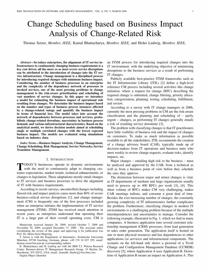
The distinction between major and minor changes is vital,as IT departments of medium and large organizations usuallyneed to process up to 400 RFCs per week [3], [4]. Thissheer volume of RFCs makes CM very challenging, makesCAB meetings tedious, and consume a great deal of time.Besides the ever-increasing number of changes, the constantlygrowing complexity of IT infrastructures further complicatesthe problem. Furthermore, classifying changes in modern ITenvironments is a challenging problem because of the multipleinterdependencies and uncertainties to manage. Consider thefollowing example, illustrated in Fig. 1, which we find in manycompanies. A business application runs several customer rela-tionship management (CRM) processes, from lead generationto sales order generation. The application itself is hosted onone or more physical resources and has dependencies to otherapplications (or services) and infrastructural components. Thescenario on the left-hand side shows a pictorial of a TivoliChange and Configuration Management Database (CCMDB)discovery [5], where Application A uses Application B. Down-time of Application B means an impact on Application A. This

IEEE TRANSACTIONS ON NETWORK AND SERVICE MANAGEMENT , VOL. X, NO. Y, MARCH 2009 2

!""#$%&'()*!*

!""#$%&'()*+*

,-.-/0-.12*

,-.-/0-31.*

!""#$%&'()*+*

,-.-/0-.12*

,-.-/0-31.*

45(%677*!* 45(%677*+*

Fig. 1: Business Process Application Dependencies

view however is not sufficient as an organization managingthe business processes will alert business users that the CRMapplication will be unavailable, which could lead to unfulfilledsales orders.

The picture on the right-hand side illustrates the morerealistic, fine-grained scenario where Application A is hostingtwo processes, e.g. lead generation and sales order generation.The actual downtime of Application B may only lead to theunavailability of lead generation but not sales order generation(which in the CRM context is a much lower risk). Furthermore,based on the fact that the affected lead generation may be alonger-running business process, one can imagine that only asubset of all running instances will be affected depending onthe state of each instance. How many instances of a particularprocess are affected further depends on the business processdemand while implementing the change, which is generallynot known a-priori but has to be approximated by meansof forecasting techniques. However, the longer the downtimefor a given service is, the more likely it is to experiencebusiness value attrition, for example due to SLA violationsand associated penalties.

In general, in today’s enterprises an increasing numberof core business processes run in an automated or semi-automated way on distributed transaction processing (DTP)systems. These systems typically have a large-scale and com-plex architecture that has grown over time.

DTP systems of medium or large companies typicallyconsist of tens of processes that are composed of hundreds ofheterogeneous, distributed IT services. Furthermore, modernIT service infrastructures are continuously transformed to-wards virtualized, shared hardware pools and Service-OrientedArchitectures (SOA) [6].

In such environments, applications as well as hardwarefunctionality can be viewed as services shared in a larger valuenetwork and invoked in the context of various processes.

Services can be described using standards such as theInterface Description Language (IDL) or the Web ServiceDescription Language (WSDL), defining for example theinterfaces of services offered as Web services, and invokedvia a suitable Internet protocol.

We distinguish between different types of services. Anatomic service in our definition is a service with a well-defined transaction boundary that provides a simple singleoperation (e.g. generate IP or assignServerName). A businessprocess is executed by invoking atomic services, other servicesthat may be composed of atomic services (e.g. short-runningtransactions), or other business processes. Furthermore, each

atomic service is executed on an IT resource.Considering the number of business processes in an en-

terprise and the complexity of the dependency network ofprocesses to invoked services, managing such an infrastructureis a highly complex task. Changes in this kind of environmentpose exceptionally high risks as the impact of failures islikely to be business-critical as many business processes mightdepend on a service. Seemingly routine tasks, such as movinga server or reconfiguring a router, might result in unplanneddowntime of core business processes. Therefore, efficient andreliable CM aimed at continuous service delivery consideringthe dependency chains is essential. We believe that CM shouldtake this level of detail into account to determine and minimizethe risk of downtime for business value generating services.

Whereas business process automation and management hasbeen a dominant topic in information systems research inrecent years, surprisingly little has been published on businessimpact and risk analysis of transitions of services involved inbusiness processes.

In this paper we focus on how to schedule service changesin complex service-oriented enterprise information systems inorder to minimize the business impact of potential change-related outage of uncertain duration. By business impact wemean the monetization of change-related impacts on depen-dent, active business process instances. A solution to thisproblem is required to automatically consider business processdemand forecasting as well as downtime estimation and itsuncertainty, as well as the dependency network from a businessprocess down to affected resources, applications, or otherservices required by business processes.

A decision model is then required to allow organizationsthe scheduling of single or multiple correlated changes withthe lowest expected overall costs.

In the remainder of this paper we propose an analyticalmodel to monetize the estimated business impact of changesand develop a change scheduling decision model based on theanalytical model.

This paper is structured as follows. In section II we reviewrelated work in this field. Section III discusses techniques toestimate and quantify operational risks of service transitionsand how to map these risks to financial loss. Subsequently,in section IV we introduce a deterministic decision modeland probabilistic extensions to determine efficient changeschedules in different business scenarios with steady andvolatile process demand. We further provide model extensionsto take into account change correlations and other sources ofrisk like violating change windows. In section V we describean approach to refine the schedule over time by updatingdemand forecasts and exploiting more reliable informationof process demand behavior and process state that becomesavailable over time. In section VI we evaluate the models byconducting simulations and we present and discuss simulationoutcomes. Section VII offers a brief summary and discussesfuture working plans.

II. RELATED WORK

In this section we review previous work in IT changerisk management and change scheduling related to the work

IEEE TRANSACTIONS ON NETWORK AND SERVICE MANAGEMENT , VOL. X, NO. Y, MARCH 2009 3

described in this paper. This paper is an extended version ofa conference paper published in the proceedings of the IEEENetwork Operations and Management Symposium 2008 [7].The novel contributions of this paper beyond those of the workdescribed in the conference version are indicated at the end ofthis section.

The definition of risk itself varies broadly according tothe specific domain one looks at. In our work we considerrisk as uncertainty of outcome’, as it is the most generaldefinition of risk [8]. In our case, the outcome is change-related cost materialized as financial loss, as we are interestedin the business impact of changes. To analyze the impact,i.e., resulting costs for the business, we draw on a two-stageapproach; first we scan for possible outcomes and quantifythese in terms of monetary consequences, and second, weweight these outcomes by their probabilities. This approachis known as probabilistic risk analysis, as introduced in [9].

In IT change management, most approaches found inthe literature, like perceived risk approaches, allow for riskanalyses that cannot be directly mapped to business or finan-cial impact, or provide general guidance to change manage-ment considering associated risk.

Publicly available best-practice ITSM frameworks and stan-dards such as the IT Infrastructure Library (ITIL) [10] orControl OBjectives for Information, and related technology(COBIT) [11], provide guidance on how to perform servicemanagement tasks and are validated across a diverse set ofenvironments and situations. Managing service changes ortransitions with respect to associated risks has recently becomea major focus of these frameworks. For example, the Officeof Government Commerce (OGC) released in the latest ITILversion 3.0 a guideline on how to manage service transitionsefficiently, in particular with regard to associated risks [8].However, ITIL and related best-practice frameworks providehigh-level guidance for tasks like managing a change, but donot provide guidance on how to do the actual change manage-ment implementation, e.g., on how to quantify, and managechange-related risks in a particular business environment.

Some commercial tools and dashboards are available toassist in managing and scheduling changes, but do not directlymap risk to expected financial impact [12]–[15].

Scheduling is a field that has received a lot of attention inthe past decades. Numerous scheduling problems have beenstudied and many solution methods have been used [16].In particular, resource constraint scheduling problems havebeen well studied [17]. Surprisingly little has been publishedon scheduling IT service changes, in particular consideringassociated risk.

Keller and Hellerstein present the CHAnge Managementwith Planning and Scheduling (CHAMPS) system to auto-mate steps in the execution of changes. The authors proposedecision models to solve different scheduling problems likemaximizing the number of changes or minimizing the costsassociated with change-related downtime. The authors assumeknowledge of cost functions for performing a change at time t,while we focus on how to derive cost functions from change-related downtime risk and uncertain process demand [18].

Goolsbey presents an approach to qualitatively evaluate IT

change risk, but does not quantitatively analyze risk [19].Closest in spirit to our work are the works by Rebouas et al.,

Trastour et al., and Sauve et al. They address the problem ofscheduling changes by minimizing the financial loss imposedby SLA violations. The authors explicitly consider uncertaintyin change implementation durations and costs resulting fromexceeding change windows [20]–[22]. Again, for minimizingfinancial loss, costs for performing a change at time t areassumed to be known, while our focus is on how to derivethese costs based on estimating the impact on dependentbusiness processes.

Our work serves to fill the gap in work addressing the quan-tification of service change-related risk to active and dependentbusiness processes, enabling the scheduling of service changeswith minimum impact on the business.

In the published conference version we focused onanalyzing the business impact of a change-related service’soutage on dependent, short-running business process instances.We considered smooth business process demand scenarios andwe assumed to have fairly reliable demand forecasts.

In this journal version we introduce and evaluate a modelfor scheduling multiple changes in the presence of volatileprocess demand for short-running as well as for more infre-quent longer-running business transactions. We further con-sider uncertain and volatile process demand behavior. Weextended the formulations of the conference version to allowfor the controlling and adjusting of scheduling plans over time,explicitly considering the stochastic nature of future demandand service downtime duration. Furthermore, we take intoaccount the progress (state) of long-running processes and weconducted more exhaustive sets of simulations based on dataof a telecommunication provider’s DTP system.

III. SERVICE TRANSITION AND ASSOCIATEDRISK TO BUSINESS PROCESSES

The goal of service transition management is to deploynew service releases into the production environment withminimum impact on the business. Implementing a change isinherently coupled with potential downtime of one or moreservices, and risk to the business.

We distinguish between unexpected and expected downtime.In the case of unexpected downtime, mostly there is nochange-related downtime but inherently a certain probabilityof an outage of unknown length. An example might be thehot deployment of an update that fails in 0.5% of casesand the previous state needs to be restored and reconfiguredmanually, which takes between five minutes and thirty minutestime where a service is unavailable. Considering expecteddowntime (e.g., average time period required for cable unplug-ging and plugging when replacing a switch), an estimator forthe average downtime duration might be known beforehand,but downtimes deviates from change to change, even thoughpossibly within tight boundaries.

From a statistics point of view, in both cases change-relateddowntime is a random variable following a certain probabilitydistribution.

As described in section I, service transition in Service-Oriented DTP systems is coupled with exceptionally high risk

IEEE TRANSACTIONS ON NETWORK AND SERVICE MANAGEMENT , VOL. X, NO. Y, MARCH 2009 4

and complexity, as there are multiple interdependencies anduncertainties to manage and many business processes mightdepend on a service. It is therefore imperative that IT organi-zations analyze and eliminate as many change-related risk aspossible by increasing the visibility of IT interdependencies.Therefore, a clear picture and a formal description of thebusiness process and service dependency structure is vital atthe beginning.

A. Dependency structure

Existing process and service definitions, for example for-malized in the Web Service Business Process Execution Lan-guage (WS-BPEL) or the Business Process Modeling Notation(BPMN), can be used to derive parts of the dependency struc-ture, although such definitions typically contain only serviceswith a certain level of abstraction from hardware functionalityand do not cover the whole dependency structure. Furthermore,they address many aspects not of immediate interest here.

To derive dependency structures, ITIL proposes the usageof a configuration management database (CMDB). In terms ofITIL, so-called configuration items (CI) should be created andcatalogued in a CMDB that acts as a repository for CIs andtheir relationships. A CI is defined as any identifiable itemthat supports business services or processes, from hardwarecomponents to business processes themselves. In the spirit ofSOA, we can map every service to a CI and vice versa.

We will now introduce a notation that is used throughoutthis paper to formalize process and service dependencies.The model parameters can be derived from information in anexisting CMDB or in business process models as long as theCIs and their relationships are described.

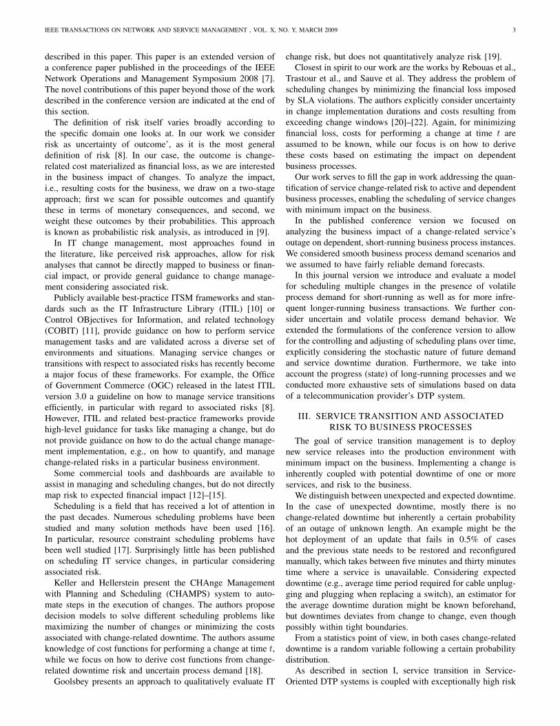
Let S := I ∪ J ∪ K be the set of all CIs, where thesubsets I , J , and K are mutually disjoint. Let I be the subsetof |I| different business process types i. Let J denote thesubset of |J | second layer service definitions j, describingan aggregated service on the layer below the business pro-cess layer. This layer represents automated workflows thatmerely string together several atomic services k where Kdenotes the set of |K| atomic services. Given all relationsuab modeling a dependency with either (a ∈ I and b ∈ J)or (a ∈ J and b ∈ K), the full dependency graph of thethree-layer system is derived (modeling four or more layers isstraightforward). A relationships uij indicates that a particularbusiness process type i uses workflow j in process step uij .We set uij := 0 if a business process i definition does notinclude an aggregated service j. In the same manner we modelthe dependencies of lower-level services by assigning atomicservice types k to aggregated services flows j correspondinglyby setting ujk to the step in j’s definition. Fig. 2 illustratesthe resulting dependency model. This dependency model pro-vides the means of automatically deriving which higher-levelservices and business processes might be affected by a specificservice downtime. However, to estimate the business impact,additional information is required, for example how costs canbe assigned to a process disruption or delay, or how manyinstances of business processes will be disrupted or delayed.

!"#$%&##'

()*+&##'

,-*.$+!'

/&)0$+&'

1*.2*#$-&''

/&)0$+&'

!"

'#"

'$"

%!#34'

%#$34'

Fig. 2: Three-Layer Service Dependency Model

B. Cost of a business process disruption or delay

The business impact in terms of costs associated withbusiness process disruptions or delays depends strongly onthe business an enterprise is running, the type of a businessprocess, the time of day, and the day of week. Prior work onestimating these costs mostly measured the direct loss of rev-enue for online companies (Web shops, online travel agencies,etc.) or other services that cannot possibly function if servicesare down [23]. For lost revenue that is directly assignable toworkload lost during a service or process failure, Walsh et al.propose simply multiplying the amount of workload that isexpected to be lost from the simulated element failures by acost-per-unit ratio [24].

However, Patterson – among others – stated that salesprocesses of such businesses are not the only ones that loseincome if the availability or performance of processes isaffected [25]. In Patterson’s model, cost is a function of lostrevenue and lost productivity, as there is for example a lossto a company in wasting employees’ time if they cannot gettheir work done. There are more, although less obvious, coststhat can be included in such a business impact model, such aspenalty payments imposed for missed deadlines, late fees foruntimely delivery, costs of opportunity of lost future revenue,or erosion of company and/or IT department reputations.

Some models like Hewlett Packard’s model of downtimecosts include the calculation of estimates of significant othercharges as mentioned above on an application-by-applicationbasis without considering service dependencies [26].

Total costs need to be considered by an organization whenservices or whole business processes are outsourced to an ITservice provider because outsourcing typically involves thetransfer of responsibility as well. The higher the estimatedloss resulting from delayed or disrupted business processeswill be, the more incentives are advised for a service supplierto mitigate downtime that may lead to disruption or delay.

A common business practice is therefore the inclusion ofService Level Agreements (SLA) in contracts between anorganization and a supplier, involving financial penalties ifagreements are missed. Therefore, from a service provider’spoint of view, the function to map delays or disruptions ofbusiness processes into costs is explicitly formalized in SLAs,

IEEE TRANSACTIONS ON NETWORK AND SERVICE MANAGEMENT , VOL. X, NO. Y, MARCH 2009 5

typically including a process’ maximum response or executiontime Li,max and the definition of penalties pi to pay onSLA violations. Depending on individual SLAs, penalties arepaid per maximum response time violation, if the number ofservice level violations during a given time span exceeds adefined threshold value, or other agreements. Note that intoday’s profit center-oriented enterprises, SLAs are typicallydefined between a company’s departments and its central ITdepartment as well. In our work we assume SLAs to be definedbeforehand and we aim at minimizing total SLA-based penaltypayments with our change-scheduling model.

C. Process demand and process state

The number of affected business process instances dependson the number of active instances and their states during achange-related service downtime. Business forecasting tech-niques are used to estimate the demand for a certain businessprocess during a particular period of time. In our conceptualmodel, for the sake of computational efficiency we divide timeinto small discrete time intervals t (t = 1, . . . , T ), wherein weassume fixed demand levels. Let Di be i’s overall demandprofile (i.e., the demand probability distributions Dit of allconsidered time intervals). Demand forecasts for time intervalt, dit, can be derived for example by setting dit to Dit’s meanvalue or to a certain percentile of Dit’s distribution.

Let ∆tdj indicate service j’s change-related downtime lengthin time intervals. Multiplying the number of expected instancesof all process types i with uij (uij > 0) during ∆tdj withassociated penalties overrates change-related costs, as not allrunning process instances will necessarily be affected.

Consider business process instances that already passed thestep invoking the changed service. These instances will not beaffected, nor is there an impact on running process instancesthat will execute the changed service after its downtime, oncethe service is again available. Furthermore, processes andservices might be queued, with a certain chance to rollbackand execute affected process instances still within time.

A procedure is described below to estimate the number ofSLA violations if queuing is not possible. Later we extendour discussion by including queuing processes and services.We start out with a deterministic model, assuming reliableknowledge of process demand and change-related downtime,followed by introducing a probabilistic model to account foruncertainty in both demand and downtime.

D. Deterministic business impact model for smooth demand

Consider an RFC for service j with a downtime ∆tdj –known a priori – starting at j’s change time tj . For esti-mating the business impact we approximate the fractions ofthe demand per dependent process type i, dp

ijt that will bepenalized (please note that the penalized demand is labeledwith subscript p) because of j’s outage. Multiplying thisnumber with a penalty payment pi, associated with each SLAviolation of a business process type i, the costs cjt of j’soutage are given in (1).

cjt =∑

i

pidpijt (1)

To estimate dpijt we proceed as follows. Because in our basic

model we assume that services cannot be queued, all processinstances executing j during time period [tj , tj + ∆tdj ] areautomatically disrupted. We assume equal arrival rates ofbusiness process requests per time interval (principle of in-difference). This assumption is tight as long as the forecastingtime intervals (timeslots) are kept small. Of interest is thedemand for a business process i not only during the change-related downtime [tj , tj + ∆tdj ] but also before tj , as runningprocess instances starting before tj might reach service jduring [tj , tj + ∆tdj ]. Let Ls

j be the execution time of servicej and let Li be i’s overall process execution duration. Weassume deterministic values for Ls

j and Li, where Li equalsthe sum of execution times of services invoked by i.

As in our basic model we assume smooth business processdemand profiles around tj , the number of active i-instancesequals dit ·Li, the demand for i per timeslot multiplied by i’sduration. Multiplying this value with the probability Ls

j/Li

that an i-instance executes j at tj , gives us an estimate forthe number of active i-instances immediately disrupted in tj .The number of i-instances reaching j in [tj , tj + ∆tdj ] is – onaverage – dit · ∆tdj , the process demands per timeslot in tjmultiplied by the downtime duration. Thus, the total expectedcost of a process’s SLA violations can be estimated using (2).

cjt =∑

i

pidit(Lsj + ∆tdj ) (2)

This cost approximation is appropriate in scenarios with rathersteady demand in [tj−max {Li,∆tdj}, tj+max {Li,∆tdown

j }]where the sum of business process instances starting in atimeslot almost equals the sum of instances finished in atimeslot. Here, the step at which a business process usesservice j is irrelevant for our calculation. Furthermore, themodel assumes that services cannot be queued and continuedat a later time.

E. Impact of queuing

We will now look at the estimated cost of changing jif queuing is supported. If queuing is supported, not allbusiness process instances that execute j during [tj , tj + ∆tdj ]are automatically disrupted, as process instances may rollback and re-execute j after tj + ∆tdj . Let Lmax

i denote i’smaximum execution time as defined in an SLA, and let bi(bi := Lmax

i − Li) represent a time buffer calculated as thedifference between the maximum and the regular executiontime of a process i if all required services are available.Obviously, if bi ≤ ∆tdj , all considered i-instances will exceedLmax

i , and if (∆tdj + Lsj) < bi, no i-instance will be delayed

or disrupted. If (∆tdj < bi < ∆tdj + Lsj), the percentage of i-

instances successfully delivered in time after a rollback andre-execution of j is given in (3).

bi −∆tdjLs

j

(3)

If bi > ∆tdj , all running i-instances invoking j in [tj , tj +∆tdj ]are deliverable in time. If bi < ∆tdj , the rate of successfully

IEEE TRANSACTIONS ON NETWORK AND SERVICE MANAGEMENT , VOL. X, NO. Y, MARCH 2009 6

delivered i-instances invoking j in [tj , tj + ∆tdj ] is bi/∆tdj .The total change-related penalty payments are given in (4).

cjt =∑

i

ditLi ·

(1−max

(0,min( bi∆td

j

Lsj, 1))

+ min(1, bi

∆tdj

)

)(4)

F. Volatile process demand

When a CAB is faced with rather volatile demand forbusiness processes, a finer-grained approach is required todetermine the number of disrupted process instances, as thenumber of process instances requested in tj might deviatewidely from the number of requests expected in precedent andsubsequent timeslots. Hence, here the process demand levelsin each timeslot and the position of j’s execution in i needsto be taken into account.

In scenarios without a queuing option, the number ofchange-related SLA violations can be estimated in the fol-lowing way. Let Li,(j−1) be i’s time required to execute allservices preceding step uij where j is invoked. Consequently,dp

ijt equals i’s total demand during [(tj − Li,(j−1)), (tj −Li,(j−1)) + Ls

j ] (instances executing j in tj) and i’s demandduring [(tj − Li,(j−1) − ∆tdj ), (tj − Li,(j−1))] (instances in-voking j during j’s outage). Hence, the total demand for ithat is penalized as a result of changing j in t, dp

ijt, is thedemand during [(tj − Li,(j−1) −∆tdj ), (tj − Li,(j−1)) + Ls

j ].By forecasting the aggregated demand during the period oftime as mentioned above (dp

ijt), total penalty payments cjt

can be estimated using (1).If queuing is a valid option, as in our basic model, we need

a fine-grained determination of dpijt. To approximate change-

related downtime costs cjt, again we forecast the processdemand during the period given in (5) and substitute the termon the left-hand side in (4), dit · Li by the resulting sum.

[(tj − Li,(j−1) −∆tdj ), (tj − Li,(j−1)) + Lsj ] (5)

G. Probabilistic demand and downtime distribution

So far, we used deterministic approximations for expectedchange-related downtime and demand levels per timeslot. Inreality, these values are stochastic variables following certainprobability distribution. Ignoring the probabilistic nature ofdemand and downtime might be acceptable for very narrowprobability distributions, but otherwise this is not advisableas it may lead to inaccurate cost estimation and poor changescheduling decision making, as described later in this paper.

Suppose an RFC for service j and a depending businessprocess i with high penalties to pay on execution time viola-tion. Let the mean change-related downtime of j, as observedin the past, be 10, but varying broadly. Suppose there is adecision to make to either start the change at t=0 or at t=50.The demand for i is expected to be slightly lower duringt=0-9 than during t=50-59 but increases rapidly from t=10onwards, while demand is expected to be of constant levelafter t=59. The deterministic model would certainly select t=0.A stochastic model explicitly taking into account uncertaintyof downtime would select t=50, which would be the betterdecision as the risk of high change-related costs is reduced.

However, putting too much stochastic information into amathematical model makes it intractable at least for mediumand large problem sizes and limits its practical applicability.Hence, to consider the stochastic nature of the variables whilekeeping the calculation computable, we draw on a stochasticformulation with simple recourse, as introduced for exampleby de Boer [27] or Birge and Louveaux [28]. The principle isillustrated in Fig. 3 with normally distributed downtime. We

!"#$%$&'&()*+,-.&()

*

! ! !!!!!!!!!!!"#$%&*

/01*

/02*

/03*

/04*

* *

/*

+#5-67,*867,*.'#(.9*

**4************000*******************-*********** * * ****************:*

Fig. 3: Probabilistic Modeling of Downtime

separate the distribution into N sequential discrete sectionsn (n=1, . . . , N ). The cumulated probability of a section isthen interpreted as one of N downtime singletons, whereaswe suppose downtime can only take these discrete values:∆tdj ∈ {∆tdj1,∆t

dj2, . . . ,∆t

djN} with certain probabilities

P (∆tdjn == ∆tdj ).Using the formulas (1) and (4), or their extensions for

volatile demand as described in the previous subsections, foreach of the N discrete downtime values ∆tdjn, the expectedcosts cjtn of changing j in t can be determined. The expectedcosts are then derived as the sum of the weighted costexpectation, computed as given in (6).

cjt =∑

n

∑i

cjtnP (∆tdj == ∆tdjn) (6)

The left part of the formula computes the costs of a changeof j in t if the downtime would be exactly ∆tdjn. The termon the right-hand side of the formula is a correction for theuncertainty (probability) in downtime: a weight. Likewise wemodel stochastic business process demand in a timeslot bycalculating change-related costs for different possible demandlevels, and weighting these demand levels with their associatedprobabilities.

For reasons of brevity, we refer below to the deterministiccost estimations in (2) and (4) even though all statements arevalid for probabilistic cost estimations as well.

Please note that additional stochastic sources exist, likeservice execution times and – as a result – process execu-tion times, which can be addressed in the same manner asstochastic downtime and demand.

IEEE TRANSACTIONS ON NETWORK AND SERVICE MANAGEMENT , VOL. X, NO. Y, MARCH 2009 7

H. Non-linear processes and multiple service invocations

The determination of change-related penalties as introducedin the previous section assumes linear business processes andservice flows with a predetermined sequence of service exe-cutions. In practice, business processes take different branchesbased on certain conditions and business process variations doexist. One branch might include a changed service while othersdo not. Hence, a finer-grained demand forecast is requiredfor each possible branch, as ignoring conditional brancheswould overrate the number of expected penalty payments.By analyzing the demand history of executed branches, adifferentiated forecast for each branch can be derived. Eachbranch can then be modeled as an individual process type.

Process definitions that involve the invocation of a service jseveral times, for example in iterative sequences, cannot be de-modulated in the same manner by defining each possible flowas a separate process, as such processes are more vulnerableto delay and disruption.

Reconsidering (2), in smooth demand scenarios we canestimate change-related costs by multiplying the costs derivedby (2) by the number of occurrences of j in a process idefinition if and only if downtime never exceeds the timelag between two j-occurrences. The same holds for costs ininfrastructures with queuing options as given in (4). In the caseof volatile demand, the interval where demand is aggregatedas given in (5) needs to be extended. One additional intervalper occurrence of j (e.g., each loop iteration) in i’s processdefinition needs to be included, where the term Li,(j−1) in (5)is adjusted for each occurrence of j in i’s definition.

If there is a certain probability that downtime overlaps withtwo or more j-occurrences, the procedure described in theprevious paragraph needs to be modified in order to avoiddouble or triple counting of penalty costs per process instance.For reasons of brevity, we sketch the principle idea of aheuristic that we apply in that case without going into detailhere. First, for each occurrence of j in a process definition weestimate change-related costs in isolation (by ignoring otheroccurrences of j). Subsequently, we employ probabilities thatdowntime overlaps two or more particular occurrences of jas weights for the costs per j-occurrence. Expected costs arethen the sum of costs for each j-occurrence.

IV. CHANGE SCHEDULING DECISION MODEL

In the next subsection, we will introduce a schedulingdecision model for uncorrelated changes. Based on this model,extensions are proposed to consider other types of opera-tional risks and costs associated with service transitions (i.e.,changes). Subsequently, we address the handling of correlatedchanges. The models aim to find optimal change timeslots withminimum resulting business impact in terms of cost.

A. Basic scheduling model

We will now introduce mathematical programming modelsto determine the schedule for a set of uncorrelated changeswith minimum expected overall service level violation costs.

We assume that a penalty is paid per SLA violation. In theprevious chapter we estimated the costs of changing a servicej in a timeslot t.

Given these estimates, finding the optimal change schedulefor uncorrelated changes is possible by scanning all timeslotsand choosing the change timeslot with the lowest expectedcosts. To formalize the decision model, we introduce a binarydecision variable xjt indicating whether j’s change is startedin t or not. Let JRFC be the set all RFCs.

The objective function, aimed at minimizing the total sumof change-related penalty payments for all i-instances invokingj is given in (7). ∑

j∈JRF C

∑i:uij>0

∑t

(cijtxjt) (7)

We set the first timeslot of our change planning period to t=0and assume to obtain JRFC before t=0. Please note that inpractice some changes – in particular urgent changes – willbe requested on a continuous time base rather than bundled.Means of addressing this are either to apply online schedulingalgorithms or to recalculate the optimization problem eachtime a new RFC is submitted, or in a certain frequency (e.g.,once an hour or once a day). In the literature, the secondprocedure is usually called optimization with rolling horizon.As we divide time into timeslots, time-related parameters areof positive integer type (tj ,∆tdj , t

∗j , bi, Li, L

sj ∈ Z

+0 ).

Penalty, cost, and demand parameter are of positive realtype (dit, dijt, pi, cijt ∈ R+

0 ).

B. Change deadlines and waiting costs

As further constraints we introduce change implementationdeadlines t∗j . Depending on the severity of a change, thereis generally an urgency associated with a change, defining adeadline when a change needs to be implemented and theservice is again available. Considering a planned, predictablechange-related downtime (e.g., a server reboot), this constraintcan be formulated using (8).∑

t≤t∗j−∆td

j

xjt = 1,∀j ∈ JRFC (8)

Equation (8) defines it as mandatory to meet change deadlines.Considering the stochastic nature of change-related servicedowntime, depending on the underlying distribution it can nolonger be guaranteed to meet deadlines and only a certainprobability can be assigned to punctual change implementa-tion. Therefore (8) is relaxed by claiming that a change mustat least start before the change deadline, as given in (9).∑

t≤t∗j

xjt = 1,∀j ∈ JRFC (9)

Note that exceeding a deadline might entail a predefinedpenalty or extra payments for each additional timeslot thata service is down, either to repair the service in the case ofunplanned downtime, or time to fulfill a change in the caseof planned downtime. Hence, the later a change is started, thehigher the expected costs of a deadline violation will be since

IEEE TRANSACTIONS ON NETWORK AND SERVICE MANAGEMENT , VOL. X, NO. Y, MARCH 2009 8

the probability of completing change fulfillments before theirdeadline will decrease continuously.

Assuming a variable penalty model where αj denotes theadditional costs per timeslot j’s change deadline is exceeded,(11) minimizes the expected overall deadline violation cost.

min∑

j∈JRF C

∑i:uij>0

∑n

∑t

(αiP (∆tdj ==∆tdjn)·max(0, xjtt+∆tdjn − t∗j )

)(10)

As in (6), we model the random variable downtime usinga stochastic formulation with simple recourse. Again, theformula computes the deadline violation costs when startinga change of j in t if the downtime would be exactly ∆tdjn,weighted by the probability that the realization of the down-time ∆tdj equals ∆tdjn. To consider deadline violation cost inthe scheduling model, formulation (11) needs to be added tothe objective function in (7).

For reasons of clarity, in the following equations we onlyassume downtime to be random; demand or service executiontimes can be modeled stochastically as well, as shown earlier.

Furthermore, the moment an RFC is submitted, there mayalready be a need felt for the change to be implemented, asthe business may suffer until this has been done. For example,this may be due to a service being unavailable, as wouldhappen if the change request was initiated as a result of anincident, or there may be other negative impact causes, likelost opportunities such as would occur for a change meant tobring in a new required service. With γj as the implicit costsof waiting one more timeslot, waiting costs are considered inthe objective functions as formulated in (11).

min(∑

j∈JRF C

∑n

∑t

(γjxjt(t+ ∆tdjn)·P (∆tdj == ∆tjnd)

)(11)

C. Change windowsTo mitigate the risk of downtime during operational working

hours, change implementations are usually restricted to a setof change windows, e.g. weekends or nighttimes. Violatinga change window restriction might have serious impacts onthe business, as that means a critical service is down attimes when this service is frequently requested. Therefore,penalties are to be paid for exceeding a change window.Let Tcj be the set of change windows w (w = 1, . . . ,W ),where each change window has an associated timeslot rangeof [tstart

jw , tendjw ]. Again, considering downtime as a random

variable, risk of change window violations increases the later achange is started in a change window. With βj quantifying thecost per timeslot a change window is exceeded for a changeof service j, and the restriction that a change must (at least)start inside a change window (tj ∈ Tcj), the formula aimed atminimizing change windows violation costs is given in (12).

min∑

j∈JRF C

∑t

(max

(0, βj(txjt + ∆tdj )−

min(tendjw : tend

jw > tj)) )

(12)

Although (12) models downtime in a deterministic way, down-time modeled as a random variable can be done as in previousformulas.

D. Dependent changes

So far in our formulations we handle multiple independentchanges. As changes might be correlated (e.g. multiple ser-vices must be changed in a mandatory order to re-engineer awhole business process), we now extend the model formulationto consider correlated or dependent changes. First, changesmight be started in a certain sequence (tj < t(j+1)), or achange must be implemented before the next change may bescheduled (tj + ∆tdj < t(j+1)). Here, the constraint in ourscheduling model is (txit < tx(j+1)t), or (txjt + ∆tdj <tx(j+1)t), respectively.

Besides a mandatory change scheduling order, changesmight be statistically correlated, for example in terms of areduction of aggregated downtime when executing changestogether. Imagine two patches to a server operating system,both requiring a reboot. On the one hand, applying thesepatches together might reduce the overall change duration,as only one reboot is required. On the other hand, forexample due to potential incompatibilities, installing bothpatches at once might result in higher risk in terms ofhigher downtime variance. Let M(∆tdj ) be the mean valueof downtime resulting from changing j, and let M(∆td(j+1))be (j + 1)’s mean change-related downtime, assuming thatj’s change is implemented before changing (j + 1). Fur-thermore, let M(∆tdj ,∆t

d(j+1)) be the mean downtime of

changing j and (j + 1) together (likewise we proceed forvariance V ). We consider two changes to j and (j + 1) ascorrelated if M(∆tdj ) + M(∆td(j+1)) 6= M(∆tdj ,∆t

d(j+1)) or

V (∆tdj ) + V (∆td(j+1)) 6= V (∆tdj ,∆td(j+1).

We treat each change item combination with significantdeviant aggregated statistical values as one single change.Whereas arbitrary statistical moments can be chosen, as anexample we focused on mean and variance. The decision tomake is to either schedule all statically dependent changesseparately or to schedule the new aggregated change instead.If the question is to either change j or (j + 1) separately or,alternatively, to implement the aggregated change (j, j + 1),the XOR constraint can be formulated as given in (13).∑

t

xjt + x(j+1)t + 2x(j,j+1) = 2 (13)

The deadline for (j, j + 1) is then set to min (t∗j , t∗(j+1)).

E. Example scheduling model formulation

In the preceding subsections we formulated componentsor model parts, which will now be assembled to derive afull scheduling decision model. Depending on infrastructureassumption (with or without queuing), business process de-mand profiles, and the amount of stochastic information to beconsidered, different model variants with different parts aresuitable. Hence, in (14) we will give an example schedulingmodel assuming smooth and predictive demand, a scenariowith queuing, and stochastic change-related downtime mod-eled as a discrete random variable. Furthermore, we considerchange window violation costs, change deadlines with costsper timeslot a deadline is exceeded, and two changes for

IEEE TRANSACTIONS ON NETWORK AND SERVICE MANAGEMENT , VOL. X, NO. Y, MARCH 2009 9

service j=2 and j=3 in a mandatory change order.

min∑

j∈JRF C

∑t:uij>0

∑n

∑t

[xjtP

(∆tdj == ∆tdjn

)·

(pidit

(Ls

j∆tdjn

))+(

max(0, βj

(txjt + ∆tdjn −min

(tendjw : tend

jw > tj))))

+(max

(0, αi(xjtt+ ∆tdjn − t∗j

))]

s.t.∑t≤t∗

jxjt = 1 ∀j ∈ JRFC

xjt ∈ {0, 1} ∀j ∈ JRFC , ∀t ≤ T

tj ,∆tdj ,∆t

djn, t

∗j , bi, t

endjw ∈ Z+

0

dit, dijt, pi, cijt, cjt, bi ∈ R+

Li, Lsj , βj , αi ∈ R+

n ∈ {1, . . . , N}

w ∈ {1, . . . ,W}

t ∈ {1, . . . , T}

(14)

The objective function minimizes the expected sum of overallcosts for service delays or disruptions, change window vio-lations, and exceeding change deadlines. The first constraintensures that each requested change is initiated before itsdeadline, the second constraint ensures the mandatory changeorder, and the subsequent constraints restrict the scope ofdecision variables and model parameters.

V. RESCHEDULING

The decision models select change timeslots with the lowestexpected overall costs based on business process demand fore-casting, assumed service downtime distributions, and penal-ties defined in SLAs. In particular if uncertainty in futureprocess demand is high, it is advisable to check and – ifnecessary – adjust a change schedule determined in t=0 beforeapproaching a time interval tj (with j ∈ JRFC). In that way,further knowledge of process demand levels and better demandpredictions can be derived to reschedule the change start times.For example, if demand forecasting in (tj-50) predicts muchhigher business process demand than initially expected, thereis a decision to make on whether to retain tj or to start thechange later or earlier.

However, when deciding to start changes later, increasingdelays or waiting costs and a higher probability of violatingchange deadline and change window restrictions has to betaken into account. In our simulations described later in thispaper we recalculate the schedule if the business processdemand forecasts computed earlier differed by more than5% from the demand predicted in order to avoid unnec-essary reschedules. Alternatively, one could reschedule at apredefined frequency or use online scheduling mechanismsinstead of recalculating complete scheduling plans. Note thatin particular when using online-scheduling mechanism, theimpact of adjusting the change time of a service on the whole

scheduling plan needs to be considered (in case of correlatedchanges).

When approaching tj , besides considering more accuratenear-term demand forecasting, we further refine our scheduleby considering the states (progress) of currently active processinstances. If in (tj-1) the percentage of running process in-stances currently executing service j exceeds our expectations,the estimated change-related costs increase and we try toderive an alternative schedule with lower costs based oncurrent cost expectations.

VI. SIMULATION

In this section, we evaluate the proposed scheduling modelsin numerous discrete event simulations based on data provi-sioned by a telecommunication provider.

We simulate scenarios with two different DTP systems,varying, non-deterministic process demand behavior, anddifferent probabilistic change-related downtime distributions.Benchmark criterion is total change-related cost when schedul-ing RFCs with the proposed deterministic model (DET) orthe probabilistic model (PROB) instead of choosing an ar-bitrary change start timeslot at the beginning of a changewindow (random selection model (RAND)). Furthermore, werelate resulting costs to the lowest possible costs, determinedby computing an optimal change schedule (OPTIMUM) expost. OPTIMUM is determined by scanning the total solutionspace with knowledge of process demand and change-relateddowntime durations and then choosing the change start timewith minimum associated costs.

The remainder of this section is structured as follows. First,the target DTP systems for our simulations are introduced.Subsequently, the simulation set-up is described. Finally, wereport and discuss simulation outcomes.

A. Target systems

As our scenario we consider two DTP systems of a largetelecommunications company. Data on system configurationas well as data on process and service dependencies is provi-sioned. Historical data on demand for processes and data onservice execution times are available via log files.

The first system, SYSTEM A, is an Enterprise ApplicationIntegration (EAI) system related to the management of thecompany’s retail customer segment. This system runs mainlyautomated business processes like billing, order entry, orderupdate, or customer data registration. Most of the processesare initiated by customers and are realized by executing trans-actions. Transactions consist of services running on distributedservers. The system runs 18 business processes involving 34transactions, which execute 61 different atomic services. Forexample, a process of adding a new customer requires theexecution of services like a credit check, the assignment ofa mobile phone number, entries in the CRM system andthe billing system, the activation of GPS services, and manymore steps. In this system, a transaction is comprised ofmultiple atomic services and a business process is comprisedof multiple transactions. The system exhibits a network ofdependencies, as one single transaction type is called by up to

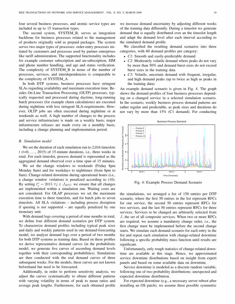
IEEE TRANSACTIONS ON NETWORK AND SERVICE MANAGEMENT , VOL. X, NO. Y, MARCH 2009 10

four several business processes, and atomic service types areincluded in up to 15 transaction types.

The second system, SYSTEM B, serves as integrationbackbone for business processes related to the managementof products originally sold as prepaid packages. The systemserves two major types of processes: order-entry processes ini-tiated by customers and processes used by partner enterpriseslike tariff administration. The supported functionality includesfor example customer subscription and un-subscription, SIMand phone number handling, and age and status verification.The complexity of SYSTEM B in terms of the number ofprocesses, services, and interdependencies is comparable tothe complexity of SYSTEM A.

In both DTP systems, business processes have stringentSLAs regarding availability and maximum execution time. Be-sides On-Line Transaction Processing (OLTP) processes, typ-ically requested and processed during daytime, long-runningbatch processes (for example churn calculations) are executedduring nighttime with less stringent SLA-requirements. How-ever, OLTP jobs are often executed during nighttime or atweekends as well. A high number of changes to the processand service infrastructure is made on a weekly basis; majorinfrastructure releases are made every on a monthly basis,including a change planning and implementation period.

B. Simulation model

We set the duration of each simulation run to 2,016 timeslotst (t=0, . . . , 2015) of 15-minute durations, i.e., three weeks intotal. For each timeslot, process demand is represented as theaggregated demand observed over a time span of 15 minutes.

We set the change windows to weekends (Friday 8pmMonday 8am) and for weekdays to nighttimes (from 8pm to8am). Change-related downtime during operational hours (i.e.,a change window violation) is penalized according to (10).By setting t∗j = 2015 ∀j ∈ JRFC we ensure that all changesare implemented within a simulation run. Waiting costs arenot considered. For OLAP processes we set the maximumexecution time to three timeslots, and for batch jobs to seventimeslots. All SLA violations – including process disruptionif queuing is not supported – are equally penalized by onemonetary unit.

With demand logs covering a period of nine months in total,we define four different demand scenarios per DTP system.To characterize demand profiles including typical peak sizesand daily and weekly patterns used in our demand-forecastingmodel, we analyze demand logs over a period of two monthsfor both DTP systems as training data. Based on these profileswe derive representative demand curves (in the probabilisticmodel, we generate five curves of ascending demand levelstogether with their corresponding probabilities). Simulationsare then conducted with the real demand curves of threesubsequent weeks. For the models, these curves are not knownbeforehand but need to be forecasted.

Additionally, in order to perform sensitivity analysis, weadjust the curves systematically to obtain different patternswith varying volatility in terms of peak to mean ratios andaverage peak lengths. Furthermore, for each obtained profile

we increase demand uncertainty by adjusting different weeksof the training data differently. During a timeslot we generatedemand that is equally distributed over an the timeslot lengthand adapt the demand level after each interval according tothe simulated demand profile.

We classified the resulting demand scenarios into threecategories, with 60 demand profiles per category:• C1: Smooth and easily-predictable demand• C2: Moderately volatile demand where peaks do not vary

by more than 50% and demand burst-sizes do not exceedburst sizes in the training data

• C3: Volatile, uncertain demand with frequent, irregular,and high demand peaks (up to twice as high as peaks inthe training data)

An example demand scenario is given in Fig. 4. The graphshows the demand profiles of four business processes depend-ing on a changed service in a selected simulation scenario.In the scenario, weekly business process demand patterns arerather regular and predictable, as peak sizes and durations donot vary by more than 15% (C1 demand). For conducting

Business Process Demand

Time (Timeslot)

Dem

and L

evel (N

um

ber

of R

equests

per

Tim

eslo

t)

0 1000 2000 3000 4000 5000 6000

2.5

3.0

3.5

4.0

Process 1

Process 4

Process 7

Process 10

!"#$%&##'()*+&##',&-.%/'

()*+&##'0'

()*+&##'1'

()*+&##'2'

()*+&##'30'

,&-.%/'4&5&6'78"-9&)'*:';&<"&#=#'>&)'?$-

&#6*=@'

''''''''''''''''''''''''''A&&B'3' ' ' ''''''''''''A&&B'C' ' ' '''''''''''A&&B'0'

?$-&'7?$-&#6*=#@'

D''''''''''''''''''CE''''''''''''''''ED'''''''''''''''2E''''''''''''''''3DD''''''

Fig. 4: Example Process Demand Scenario

the simulations, we arranged a list of 150 entries per DTPscenario, where the first 50 entries in the list represent RFCsfor one service, the second 50 entries represent RFCs fortwo services, and the last 50 entries represent RFCs for threeservices. Services to be changed are arbitrarily selected fromJ , the set of all composite services. When two or more RFCsare required, we assume a mandatory change order, i.e., thefirst change must be implemented before the second changestarts. We simulate each demand scenario for each entry in thelist and repeat each simulation with change-related downtimefollowing a specific probability mass function until results aresignificant.

Unfortunately, only rough statistics of change-related down-time are available at this stage. Hence, we approximatedservice downtime distributions based on insight from expertpanels and based on some available data on downtime.

Service downtime is modeled as a discrete random variable,following one of two probability distributions: unexpected andexpected downtime distribution.

For expected downtime (e.g., a necessary server reboot afterinstalling an OS patch), we assume three possible symmetric

IEEE TRANSACTIONS ON NETWORK AND SERVICE MANAGEMENT , VOL. X, NO. Y, MARCH 2009 11

Binomial distributions (PLANNED 1 - PLANNED 3) with amean of three, four, or five timeslots with increasing variance,where downtime singletons could take values out of [0,6],[0,8], or [0,10] time intervals. As an example with a meandowntime of three time intervals, and singletons in [0,6], onthe right-hand side of Fig. 5 the Binomial(6, 0.5) probabilitydistribution is depicted.

For unexpected downtime we consider a fat tail probabilitydistribution as no change-related downtime usually occurs, ex-cept in some cases where then time is required for reparation.We use three Zipf-Mandelbrot distributions (Unplanned 1Unplanned 3) with different variance, as we parameterize thedistributions with population sizes of seven, nine or eleventimeslots, a power exponent of three, and zero shifts (theleftmost singleton is set to zero instead of one). On the left-hand side of Fig. 5, an unexpected downtime distribution witha population size of seven (0-6 timeslots), a power exponentof three and zero shift is depicted.

DET is parameterized with the median downtime andwith mean demand per timeslot, while PROB minimizesthe weighted expected outcome for all possible downtimedurations for ten possible demand scenarios. According to

!!"!!!!!!!!!!!!###!!!!!!!!!!!!!!!!!!!!!!!!!!!!!!!!!!!!!!!!!!!!!!!!!!!!!!!!!!!!!!!!!!!!!!!!$!

%!

! !

"!

"#&!

! !

"!

!!"!!!!!!!!!!!!###!!!!!!!!!!!!!!!!!!!!!!!!!!!!!!!!!!!!!!!!!!!!!!!!!!!!!!!!!!!!!!!!!!!!!!$!

Fig. 5: Planned versus Unplanned Downtime Probability

the available log-files, service execution times vary only in-between tight boundaries and in large set of preliminarysimulations, solution qualities of the models did not sig-nificantly differ whether execution times were modeled asrandom variables or deterministic values. Hence, to keep themodels computationally tractable, we model service executiontimes as deterministic by taking their means. Please note thatthe validity of this proceeding needs to be re-checked whenconsidering target systems with a higher variance in serviceexecution times.

Within one simulation run, for all changes we assume equaldowntime probability distributions.

Although queuing is used in the company’s DTP system,we repeat all simulations without a queuing option.

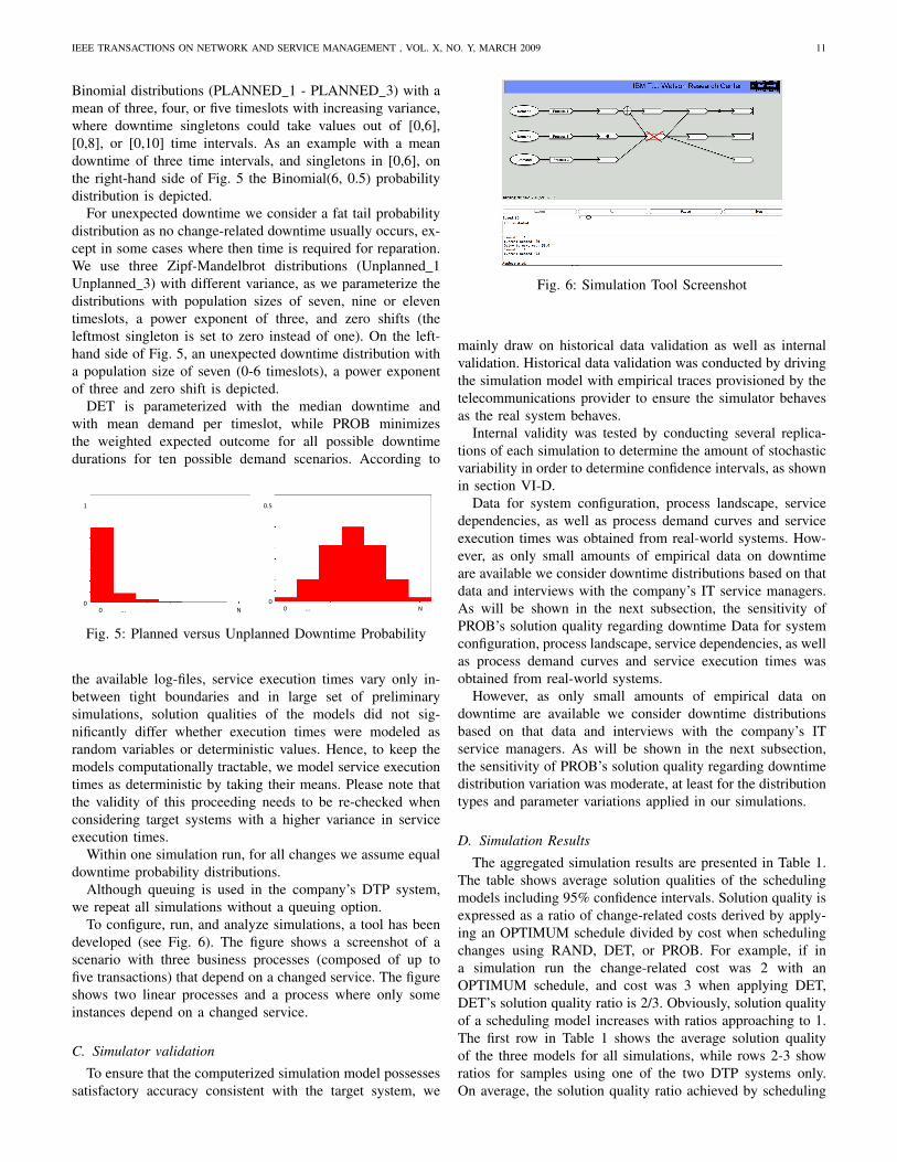
To configure, run, and analyze simulations, a tool has beendeveloped (see Fig. 6). The figure shows a screenshot of ascenario with three business processes (composed of up tofive transactions) that depend on a changed service. The figureshows two linear processes and a process where only someinstances depend on a changed service.

C. Simulator validation

To ensure that the computerized simulation model possessessatisfactory accuracy consistent with the target system, we

Fig. 6: Simulation Tool Screenshot

mainly draw on historical data validation as well as internalvalidation. Historical data validation was conducted by drivingthe simulation model with empirical traces provisioned by thetelecommunications provider to ensure the simulator behavesas the real system behaves.

Internal validity was tested by conducting several replica-tions of each simulation to determine the amount of stochasticvariability in order to determine confidence intervals, as shownin section VI-D.

Data for system configuration, process landscape, servicedependencies, as well as process demand curves and serviceexecution times was obtained from real-world systems. How-ever, as only small amounts of empirical data on downtimeare available we consider downtime distributions based on thatdata and interviews with the company’s IT service managers.As will be shown in the next subsection, the sensitivity ofPROB’s solution quality regarding downtime Data for systemconfiguration, process landscape, service dependencies, as wellas process demand curves and service execution times wasobtained from real-world systems.

However, as only small amounts of empirical data ondowntime are available we consider downtime distributionsbased on that data and interviews with the company’s ITservice managers. As will be shown in the next subsection,the sensitivity of PROB’s solution quality regarding downtimedistribution variation was moderate, at least for the distributiontypes and parameter variations applied in our simulations.

D. Simulation Results

The aggregated simulation results are presented in Table 1.The table shows average solution qualities of the schedulingmodels including 95% confidence intervals. Solution quality isexpressed as a ratio of change-related costs derived by apply-ing an OPTIMUM schedule divided by cost when schedulingchanges using RAND, DET, or PROB. For example, if ina simulation run the change-related cost was 2 with anOPTIMUM schedule, and cost was 3 when applying DET,DET’s solution quality ratio is 2/3. Obviously, solution qualityof a scheduling model increases with ratios approaching to 1.The first row in Table 1 shows the average solution qualityof the three models for all simulations, while rows 2-3 showratios for samples using one of the two DTP systems only.On average, the solution quality ratio achieved by scheduling

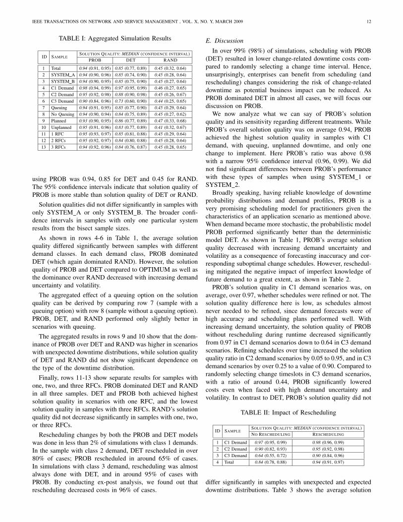
IEEE TRANSACTIONS ON NETWORK AND SERVICE MANAGEMENT , VOL. X, NO. Y, MARCH 2009 12

TABLE I: Aggregated Simulation Results

ID SAMPLESOLUTION QUALITY: MEDIAN (CONFIDENCE INTERVAL)

PROB DET RAND

1 Total 0.94 (0.91, 0.95) 0.85 (0.77, 0.89) 0.45 (0.32, 0.64)2 SYSTEM A 0.94 (0.90, 0.96) 0.85 (0.74, 0.90) 0.45 (0.28, 0.64)3 SYSTEM B 0.94 (0.90, 0.95) 0.85 (0.75, 0.90) 0.45 (0.27, 0.64)4 C1 Demand 0.98 (0.94, 0.99) 0.97 (0.95, 0.99) 0.46 (0.27, 0.65)5 C2 Demand 0.95 (0.92, 0.98) 0.88 (0.90, 0.98) 0.45 (0.26, 0.67)6 C3 Demand 0.90 (0.84, 0.96) 0.73 (0.60, 0.90) 0.44 (0.25, 0.65)7 Queuing 0.94 (0.91, 0.95) 0.85 (0.77, 0.90) 0.45 (0.29, 0.64)8 No Queuing 0.94 (0.90, 0.94) 0.84 (0.75, 0.89) 0.45 (0.27, 0.62)9 Planned 0.93 (0.90, 0.95) 0.86 (0.77, 0.89) 0.47 (0.33, 0.68)10 Unplanned 0.95 (0.91, 0.96) 0.83 (0.77, 0.89) 0.41 (0.32, 0.67)11 1 RFC 0.95 (0.93, 0.97) 0.85 (0.81, 0.88) 0.45 (0.29, 0.64)12 2 RFCs 0.95 (0.92, 0.97) 0.84 (0.80, 0.88) 0.45 (0.28, 0.64)13 3 RFCs 0.94 (0.92, 0.96) 0.84 (0.76, 0.87) 0.45 (0.28, 0.65)

using PROB was 0.94, 0.85 for DET and 0.45 for RAND.The 95% confidence intervals indicate that solution quality ofPROB is more stable than solution quality of DET or RAND.

Solution qualities did not differ significantly in samples withonly SYSTEM A or only SYSTEM B. The broader confi-dence intervals in samples with only one particular systemresults from the bisect sample sizes.

As shown in rows 4-6 in Table 1, the average solutionquality differed significantly between samples with differentdemand classes. In each demand class, PROB dominatedDET (which again dominated RAND). However, the solutionquality of PROB and DET compared to OPTIMUM as well asthe dominance over RAND decreased with increasing demanduncertainty and volatility.

The aggregated effect of a queuing option on the solutionquality can be derived by comparing row 7 (sample with aqueuing option) with row 8 (sample without a queuing option).PROB, DET, and RAND performed only slightly better inscenarios with queuing.

The aggregated results in rows 9 and 10 show that the dom-inance of PROB over DET and RAND was higher in scenarioswith unexpected downtime distributions, while solution qualityof DET and RAND did not show significant dependence onthe type of the downtime distribution.

Finally, rows 11-13 show separate results for samples withone, two, and three RFCs. PROB dominated DET and RANDin all three samples. DET and PROB both achieved highestsolution quality in scenarios with one RFC, and the lowestsolution quality in samples with three RFCs. RAND’s solutionquality did not decrease significantly in samples with one, two,or three RFCs.

Rescheduling changes by both the PROB and DET modelswas done in less than 2% of simulations with class 1 demands.In the sample with class 2 demand, DET rescheduled in over80% of cases; PROB rescheduled in around 65% of cases.In simulations with class 3 demand, rescheduling was almostalways done with DET, and in around 95% of cases withPROB. By conducting ex-post analysis, we found out thatrescheduling decreased costs in 96% of cases.

E. Discussion

In over 99% (98%) of simulations, scheduling with PROB(DET) resulted in lower change-related downtime costs com-pared to randomly selecting a change time interval. Hence,unsurprisingly, enterprises can benefit from scheduling (andrescheduling) changes considering the risk of change-relateddowntime as potential business impact can be reduced. AsPROB dominated DET in almost all cases, we will focus ourdiscussion on PROB.

We now analyze what we can say of PROB’s solutionquality and its sensitivity regarding different treatments. WhilePROB’s overall solution quality was on average 0.94, PROBachieved the highest solution quality in samples with C1demand, with queuing, unplanned downtime, and only onechange to implement. Here PROB’s ratio was above 0.98with a narrow 95% confidence interval (0.96, 0.99). We didnot find significant differences between PROB’s performancewith these types of samples when using SYSTEM 1 orSYSTEM 2.

Broadly speaking, having reliable knowledge of downtimeprobability distributions and demand profiles, PROB is avery promising scheduling model for practitioners given thecharacteristics of an application scenario as mentioned above.When demand became more stochastic, the probabilistic modelPROB performed significantly better than the deterministicmodel DET. As shown in Table 1, PROB’s average solutionquality decreased with increasing demand uncertainty andvolatility as a consequence of forecasting inaccuracy and cor-responding suboptimal change schedules. However, reschedul-ing mitigated the negative impact of imperfect knowledge offuture demand to a great extent, as shown in Table 2.

PROB’s solution quality in C1 demand scenarios was, onaverage, over 0.97, whether schedules were refined or not. Thesolution quality difference here is low, as schedules almostnever needed to be refined, since demand forecasts were ofhigh accuracy and scheduling plans performed well. Withincreasing demand uncertainty, the solution quality of PROBwithout rescheduling during runtime decreased significantlyfrom 0.97 in C1 demand scenarios down to 0.64 in C3 demandscenarios. Refining schedules over time increased the solutionquality ratio in C2 demand scenarios by 0.05 to 0.95, and in C3demand scenarios by over 0.25 to a value of 0.90. Compared torandomly selecting change timeslots in C3 demand scenarios,with a ratio of around 0.44, PROB significantly loweredcosts even when faced with high demand uncertainty andvolatility. In contrast to DET, PROB’s solution quality did not

TABLE II: Impact of Rescheduling

ID SAMPLESOLUTION QUALITY: MEDIAN (CONFIDENCE INTERVAL)NO RESCHEDULING RESCHEDULING

1 C1 Demand 0.97 (0.95, 0.99) 0.98 (0.96, 0.99)2 C2 Demand 0.90 (0.82, 0.93) 0.95 (0.92, 0.98)3 C3 Demand 0.64 (0.55, 0.72) 0.90 (0.84, 0.96)4 Total 0.84 (0.78, 0.88) 0.94 (0.91, 0.97)

differ significantly in samples with unexpected and expecteddowntime distributions. Table 3 shows the average solution

IEEE TRANSACTIONS ON NETWORK AND SERVICE MANAGEMENT , VOL. X, NO. Y, MARCH 2009 13

quality of RAND, DET, and PROB in samples with onlyexpected downtime distributions with increasing variance fromPLANNED 1 to PLANNED 3 (lines 1-3). Lines 4-6 showthe average solution quality of the models in simulations withunexpected downtime distributions, with increasing variancefrom UNPLANNED 1 to UNPLANNED 3.

As can be seen, PROB dominated DET and RAND inall samples independently of downtime distributions. As dis-cussed in section III.G, deterministic models perform worsewhen probability distributions are broadened and effects donot scale linearly with realizations of a random variable. Cor-respondingly, DET’s solution quality decreased by 0.026 whencomparing the sample PLANNED 1 and PLANNED 2, whilePROB’s average solution quality decreases by 0.006 only –likewise when comparing PLANNED 2 and PLANNED 3.In samples with unplanned downtime distributions, the de-crease ratio was around 0.045 for DET and 0.01 for PROB.In general, although better performance is expected when

TABLE III: Impact of Downtime Distributions

ID SAMPLESOLUTION QUALITY: MEDIAN (CONFIDENCE INTERVAL)

PROB DET RAND

1 PLANNED 1 0.95 (0.92, 0.96) 0.87 (0.77, 0.89) 0.45 (0.31, 0.62)2 PLANNED 2 0.95 (0.91, 0.96) 0.85 (0.76, 0.89) 0.45 (0.29, 0.63)3 PLANNED 3 0.94 (0.91, 0.96) 0.82 (0.72, 0.89) 0.44 (0.29, 0.64)4 UNPLANNED 1 0.96 (0.93, 0.97) 0.87 (0.79, 0.88) 0.46 (0.32, 0.64)5 UNPLANNED 2 0.95 (0.91, 0.97) 0.85 (0.77, 0.88) 0.45 (0.30, 0.65)6 UNPLANNED 3 0.94 (0.90, 0.97) 0.83 (0.71, 0.86) 0.44 (0.30, 0.64)

stochastic influences are considered, often the benefits arelow and stochastic modeling is not worth the effort; a well-known example is seat inventory control in airline networkrevenue management. Based on the results of our simulations,in the case of the business impact of change-related downtime,probabilistic modeling does significantly lower the costs.

Comparing PROB’s solution quality in samples with one,two, or three RFCs, PROB’s simulation results did not exhibitsignificant differences for different numbers of RFCs in C1or C2 demand scenarios. In C3 scenarios, PROB’s solutionquality decreased (although moderately) with the number ofRFCs to fulfill, as inaccuracies in demand forecasting impactsthe solution quality several times.

F. Handling the computational complexity

The scheduling decision problem as formulated in our workis proven to be strongly NP-hard. Hence, the problem isonly computationally tractable for problem instances up toa certain size, in particular as the complexity grows withT, I, J,K,N,W, and JRFC .

However, for uncorrelated changes we determined thechange-related costs of changing a service j in time inter-val t by only considering timeslots which could potentiallybe affected by a service’s downtime (i.e., the range of thedowntime random variable). For this reason we were able toefficiently parallelize the computation to 16 standard Intel DualCore 2.4 MHz computers and run one simulation within lessthan 30 seconds. For simulations with a mandatory change

order we first divided the simulation time period into 16sub-periods, where each computer was instructed to choose atimeslot within a particular sub-period as change timeslot forthe first change and to solve the problem with this restriction.Choosing the result with the lowest expected cost then derivedthe solution. Simulations with three changes in a mandatorychange order are run within a period of four minutes.

However, considering broader downtime distributions hasa huge impact on the computational time required to solvea problem. For example, simulations assuming unplanneddowntime distribution with a range of 100 timeslots requiredaround 26 minutes for uncorrelated changes, and around threehours for correlated changes. Therefore, to solve probleminstances with larger sets JRFC , in particular with correlatedchanges to implement, and broader change-related downtimedistributions, the amount of considered stochastic informationcan be reduced, timeslots may be coarsened, and heuristicsmay be applied, for example to pre-select promising changetimeslot candidates.

VII. SUMMARY AND OUTLOOK

In this paper we introduced a probabilistic model foranalyzing the business impact of changes in a network ofservices. We analyzed change-related operational risks toactive business process instances and techniques to relate theserisks to financial metrics. Based on the analytical model, wedeveloped a decision model to schedule service changes in away to reduce total expected change-related costs.

In extensive sets of simulations based on industry data, weevaluated the efficiency of the model in various scenarios withtwo different DTP systems, different downtime probabilitydistributions, different numbers of services to be changed,and uncertain process demand behavior. Simulation outcomesindicate that the proposed model schedules changes withresulting costs approaching the minimum costs theoreticallypossible if future process demand is easily-predictable andchange-related downtime distributions are known; by refiningscheduling plans over time, the scheduling model still achievedsignificant cost savings even in scenarios with highly volatiledemand that was hard to predict. Although the solution qualitydecreased with demand uncertainty and the number of RFCs,the sensitivity was moderate. In no sample did PROB’s costsexceed the minimum costs by more than 11%, which indicatesrobustness. This robustness should make the scheduling modela useful tool in supporting practitioners in their decisionmaking of how to schedule changes.

To the best of our knowledge, our work is the first toformally quantify the risk of changing services to the business(processes), or to derive decision models that allow organiza-tions to schedule service changes with minimum total expectedbusiness impact.

In order to make the model usable for practitioners to sup-port their change-scheduling decision making, besides processdemand forecasting, which can usually be done with sufficientaccuracy, reliable estimators for change-related downtime dis-tributions are required to parameterize the models. This infor-mation is usually not available to hand in organizations and

IEEE TRANSACTIONS ON NETWORK AND SERVICE MANAGEMENT , VOL. X, NO. Y, MARCH 2009 14

first need to be collected based on empirical observation. Intarget systems with more variable service execution times thanin the studied DTP systems, the sensitivity of PROB’s solutionquality to the variance must be analyzed prior to applying itin such scenarios. In particular in semi-automated processeswith human working tasks such as interactive workflows, theexecution times of services usually vary broadly. Reliabledata needs to be collected in order to estimate probabilitydistributions of service execution times.

In the future, we plan to apply the models as a decisionsupport tool for change scheduling in selected businesses.Future working plans also include more exhaustive sets ofsimulations including manual or semi-automated business pro-cesses with stochastic service execution times. To keep themodel computationally tractable and therefore applicable inpractice for larger scenarios, we will work on meta-heuristicsand change timeslot pre-selection algorithms.

REFERENCES

[1] J. P. Sauve, R. A. Santos, R. R. Almeida, and J. A. B. Moura, “Onthe risk exposure and priority determination of changes in it servicemanagement,” in Managing Virtualization of Networks and Services.Berlin/Heidelberg: Springer, 2007, vol. 4785, pp. 147–158.

[2] OGC, Service Support (It Infrastructure Library Series). London, UK:The Stationery Office, 2000.

[3] “The bottom line project. it change management challenges – results of2006 web survey,” Computing Systems Department, Federal Universityof Campina Grande, Tech. Rep. DSC005-06, 2006.

[4] OGC, “Itil change management maturity benchmark study,” EvergreenConsulting, Tech. Rep., 2006.

[5] IBM, “Tivoli change and configuration man-agement database,” 2009, [Online]. Available:http://www.ibm.com/software/tivoli/products/ccmdb/.

[6] O. Huehn and C. Markl, “Performance modeling for sla-compliantbut cost-effective it-service provisioning,” in Proc. 17th Workshop onInformation Technology and Systems (WITS), Montreal, Canada, 2007.

[7] T. Setzer, K. Bhattacharya, and H. Ludwig, “Decision support for servicetransition management,” in Proc. 11th IEEE Network Operations andManagement Symposium (NOMS), Salvador, Brazil, 2008.

[8] OGC, Management of Risk, Guidance for Practioners. London, UK:The Stationery Office, 2007.

[9] S. Kaplan and B. J. Garrick, “On the quantitative definition of risk,” inRisk Analysis, 1981, vol. 1, pp. 11–27.

[10] OGC, “Official itil website,” 2009, [Online]. Available: http://www.best-management-practice.com/IT-Service-Management-ITIL.

[11] IT-Governance-Institute, COBIT 4.1. Isaca, 2007.[12] IBM, “It service management - change and configuration management:

Reducing risk by understanding your infrastructure.” 2008, [Online].Available: http://www-03.ibm.com/solutions/tsolutions/doc/.

[13] Cisco, “Business management case study: How cisco it usessoftware configuration management to minimize business,”2007, [Online]. Available: http://www.cisco.com/web/about/ciscoitatwork/casestudies/business management dl2.html.

[14] BMC, “Bmc remedy change manage-ment dashboard,” 2009, [Online]. Available:http://www.bmc.com/products/documents/25/43/62543/62543.pdf.

[15] Hewlett-Packard, “Hp release control software,” 2009, [Online]. Avail-able: https://h10078.www1.hp.com.

[16] M. Pinedo, Scheduling: Theory, Algorithms, and Systems. Prentice Hall,2001.

[17] E. Demeulemeester and W. Herroelen, “A branch-and-bound procedurefor the generalized resource-constrained project scheduling problem,”Operations Research, vol. 45, no. 2, p. 201212, 1997.

[18] A. Keller, J. Hellerstein, J. Wolf, K.-L. Wu, and V. Krishnan, “Thechamps system: change management with planning and scheduling,” inProc. IEEE Network Operations and Management Symposium (NOMS),Seoul, Korea, 2004.

[19] J. Goolsbey, “Risk-based it change management,,” Pacific NorthwestNational Laboratory - IT Services Division, Tech. Rep., 2007.

[20] R. Rebouas, J. Sauv, A. Moura, C. Bartolini, and D. Trastour, “Adecision support tool for optimizing scheduling of it changes,” inProc. 10th IFIP/IEEE Symposium on Integrated Management, Munich,Germany, 2007.

[21] D. Trastour, M. Rahmouni, and C. Bartolini, “Activity-based schedul-ing of it changes,” in Inter-Domain Management - Lecture Notes inComputer Science. Berlin/Heidelberg, Germany: Springer, 2007, vol.4543/2007, pp. 73–84.

[22] J. Sauve, R. Santos, R. Reboucas, A. Moura, and C. Bartolini, “Changepriority determination in it service management based on risk exposure,”IEEE Transactions on Network and Service Management, vol. 5, no. 3,pp. 178–187, 2008.

[23] R. Kembel and R. Cummings, “Fibre channel: A comprehensive intro-duction,” Northwest Learning Association, Tech. Rep., 2007.

[24] J. Walsh, A. Rockall, and A. Sudarsky, “Method and apparatus toestimate downtime and cost of downtime in an information technologyinfrastructure,” U.S. Patent 20030187967, March 2002.

[25] D. A. Patterson, “A simple way to estimate the cost of downtime,” inProc. 16th System Administration Conference LISA, Philadelphia, USA,2002.

[26] “How to calculate cost of downtime,” Silverton Consulting, Tech. Rep.,2007, [Online]. Available: email: info@silvertonconsulting.com.

[27] S. V. d. Boer, R. Freling, and N. Piersma, “Stochastic programming formultiple-leg network revenue management,” ORTEC Consultants, Tech.Rep., 1999.

[28] J. R. Birge and F. Louveaux, Introduction to Stochastic Programming.New York, USA: Springer, 1997.

Thomas Setzer received his Masters degree inBusiness Engineering from the University of Karl-sruhe, Germany, and his Ph.D. degree in InformationSystems from the Technische Universitat Munchen(TUM), Germany. He worked as an engineer forthe European Parliament and Cinebank Media. Heis currently working at TUM as assistant professoron IT Management topics, in particular data cen-ter virtualization and automation. Thomas won theINFORMS ISS Design Science Award 2008 and hiswork is funded by the German Research Foundation.

Kamal Bhattacharya graduated with a PhD inTheoretical Physics from Gottingen University, Ger-many. Currently Kamal manages a team at IBMResearch exploring new ideas in the area of ITOptimization. His research focuses on topics arounddata center consolidation, application migration, andbusiness value driven strategies for IT Service Man-agement. Prior to joining IBM Research he has beenworking as an IT architect at IBM Global Servicesand received two Outstanding Tech. Achievementawards and several IBM Research Division awards.

Heiko Ludwig received his Masters and PhD de-grees from the University of Bamberg, Germany.He is a Research Staff Member at IBMs T.J. Wat-son Research Center. He is working on issues ofservice management and service platforms, primar-ily managing large-scale, loosely-coupled, cross-domain distributed systems, including service out-sourcing and cloud computing. He has publishednumerous papers and articles and serves as editorand conference organizer in various capacities.