Embed Size (px)
Citation preview
Using Matrix Approximation for High-Dimensional Discrete OptimizationProblems: Server Consolidation based on Cyclic Time-Series Data
T. Setzera, M. Bichlerb
aKarlsruhe Institute of Technology, Englerstraße 14, 76131 Karlsruhe, GermanybTechnische Universitat Munchen, Boltzmannstraße 3, 85748 Garching, Germany, [email protected]
Abstract
We consider the assignment of enterprise applications in virtual machines to physical servers, also known as server
consolidation problem. Data center operators try to minimize the number of servers, but at the same time provide suf-
ficient computing resources at each point in time. While historical workload data would allow for accurate workload
forecasting and optimal allocation of enterprise applications to servers, the volume of data and the large number of
resulting capacity constraints in a mathematical problem formulation renders this task impossible for any but small
instances. We use singular value decomposition (SVD) to extract significant features from a large constraint matrix
and provide a new geometric interpretation of these features, which allows for allocating large sets of applications
efficiently to physical servers with this new formulation. While SVD is typically applied for analytical purposes like
time series decomposition, noise filtering, or clustering, in this paper features are used to transform the original al-
location problem in a low-dimensional integer program with only the extracted features in a much smaller constraint
matrix. We evaluate the approach using workload data from a large Data center and show that it leads to high solution
quality, but at the same time allows for solving considerably larger problem instances than what would be possible
without data reduction and model transform. The overall approach can also be applied to other large integer problems,
as they can be found in applications of multiple or multi-dimensional knapsack or bin packing problems.
Keywords: Matrix Approximation, Multi-Dimensional Packing, Server Consolidation, Dimensionality Reduction
1. Introduction
Today’s larger data centers are typically hosting thousands of enterprise applications from various customers such
as Enterprise Resource Planning (ERP) modules or database applications with different workload characteristics. The
underlying IT infrastructures may contain hundreds of physical servers and various other hardware components. There
is even a trend to increase the size of data centers to leverage economies of scale in their operation (Digital Realty
Trust 2010).
To reduce the number of required servers, server virtualization has been increasingly adopted during the past few
years (Hill et al. 2009). Server virtualization refers to the abstraction of hardware resources and allows the hosting of
Email addresses: [email protected] (T. Setzer), [email protected] (M. Bichler)
Preprint submitted to EJOR May 11, 2012
multiple virtual machines (VM) including business applications plus underlying operating system on a single physical
server. The capacity of a physical server is then shared among the VMs, leading to increased utilization of physical
servers. While traditional capacity planning in Operations Research relies on queuing theory or simulation to predict
the performance of a single dedicated system given available resources and resource demands (Huhn et al. 2010), new
challenges arise in the capacity planning for virtualized data centers.
We consider the problem of assigning enterprise applications with time-varying demands for multiple hardware re-
sources such as CPU, memory, or I/O bandwidth efficiently to servers with finite capacities. In this domain, economic
efficiency means the use of computing resources so as to minimize the number of servers required to provide a given
set of VMs. Applications installed in VMs must get enough resources in order to conform to pre-defined service level
agreements. This new capacity planning problem has been described as the server consolidation problem (Speitkamp
and Bichler 2010).
1.1. Server Consolidation
Data centers usually measure resource utilization for each VM and for each physical server. For example CPU
utilization and allocated memory of a server are typically logged in five-minute intervals. Such log data can then be
used for characterizing and predicting future resource demands and determining efficient VM allocations. Industry
practice usually follows simple approaches to consolidate servers based on peak workloads observed in the past.
For example, administrators collect maximum VM demands for various resources over several weeks and derive a
respective VM demand vector. VMs are then assigned to a physical server at a time until the demand exceeds the
capacity.
Many enterprise applications exhibit predictable workloads with daily or weekly seasonalities (Parent 2005, Rolia
et al. 2005). Enterprise applications with predictable workloads are actually the prime candidates for server consol-
idation projects as these allow for reliable resource planning and high potential server savings. For example, email
servers typically face high loads in the morning and after the lunch break when most employees download their emails,
payroll accounting is often performed at the end of the week, while workload of a data warehouse server has a daily
peak very early in the morning when managers typically access their reports.
The problem can be modelled using a multi-dimensional bin-packing (MBP) problem formulation. We will briefly
introduce the formulation as a succinct description of the server consolidation problem, as it will provide a basis for
the contribution in this paper. Suppose that we are given J VMs j = 1, . . . , J to be hosted by I servers i = 1, . . . , I
or fewer. Different types of resources k = 1, . . . ,K such as CPU, I/O, or main memory may be considered and each
server has a certain capacity sik of each resource k. yi is a binary decision variable indicating if server i is used, ci
describes the cost of a server (for example, energy costs per hour), and the binary decision variable xi j indicates which
VM j is allocated to which server i. The planning period is divided into time intervals indexed by t = 1, . . . ,T . These
intervals might be minutes or hours per day if we have daily periodicity. Let r jkt be the capacity that VM j requires of
resource k in time period t. The server consolidation problem can now be formulated as the MBP in (1).
2
min∑i
ci · yi
s.t.∑i≤I
xi j = 1 ∀ j ≤ J∑j≤J
r jkt · xi j ≤ sik · yi ∀i ≤ I,∀k ≤ K,∀t ≤ T
yi, xi j ∈ {0, 1} ∀i ≤ I,∀ j ≤ J
(1)
The objective function minimizes total server costs. The first set of constraints ensures that each VM is allocated
to one of the servers, and the second set of constraints ensures that the aggregated resource demand of multiple VMs
does not exceed a server’s capacity per host server, time interval, and resource type. As we will show in Section 4,
r jkt can typically be estimated with sufficient quality from workload data.1
Speitkamp and Bichler (2010) have shown that the consideration of daily workload cycles using an MBP formu-
lation can lead to 31% savings in physical servers. These results are only based on smaller instances of up to 50
Enterprise Resource Planning (ERP) applications or around 200 Web applications, but considering only CPU and
aggregating the workload data to 15-minute time intervals. Although the consideration of memory and I/O is essential
in most projects, the resulting MIPs would not be tractable except for small problem sizes with ten or twenty VMs.
When daily workload cycles are assumed and resource requirements for all five-minute time intervals per day are con-
sidered, resource demand behavior is described by 288 distinct time intervals (T = 288). So the number of resource
constraints in (1) grows with O(T KI) and there are O(IJ) binary variables.
Linear programming-based heuristics, which allow for the consideration of important technical allocation con-
straints have also been evaluated, but did not lead to a significant increase in scaleability. Although server consol-
idation based on mathematical programming has shown to yield considerable savings in server cost, this curse of
dimensionality is a barrier not only to this but any practical application in data centers, where often hundreds of VMs
need to be considered. The problem is important for IT (information technology) service managers, because data
centers regularly need to assign or reassign a set of VMs to a new hardware infrastructure.
1.2. Solving High-Dimensional Resource Allocation Problems
The sheer volume of workload data of hundreds of VMs is a challenge when applying mathematical optimization
to solve the resource allocation problem. There is a significant literature on solving large-scale integer programs with
1Nowadays, VM managers such as VMWare or Xen allow for a dynamic reallocation of VMs during runtime (Clark et al. 2005). As of now,
there is little understanding of the dynamics and the stability of the overall system that might emerge as a result of automated reallocations of VMs.
Such reallocations require a significant amount of CPU and memory resources on the physical servers as well as network bandwidth. Repeated
daily demand peaks might lead to many reallocations for short time periods when dynamic reallocations are used. Therefore, stable allocations of
virtual machines to servers, which do not require reassignments during a defined period of time, are a preferred means of capacity management by
most IT (information technology) service managers.
3
many variables which consist of sparse, specially structured constraint matrices using techniques such as column gen-
eration. An overview of such techniques can be found in Barnhart et al. (1996). In the server consolidation problem,
however, the constraint matrix has many constraints rather than many variables. Furthermore, the constraint matrix
is not sparse and it does not exhibit a special block diagonal structure as is required for Danzig-Wolfe composition
algorithms and branch-and-price approaches.
A literature review of Wascher et al. (2007) reveals that research on cutting and packing problems still is rather
traditionally oriented, stressing areas which include clearly-defined standard problems with one, two, or (sometimes)
three dimensions. Heuristics and approximations with good computational results have been developed for specific
packing problems with one up to three dimensions (Lodi et al. (1999), Faroe et al. (2003), Grainic et al. (2009)).
Polynomial time approximation schemes (PTAS) have also been developed for MBP, but the gaps between upper
and lower bounds on the solution quality increase with the number of dimensions, which limits their applicability
to problems with a low number of dimensions. For d-dimensional vector packing, for instance, no polynomial-time
approximations are at hand with performance guarantees better than ln(d) + 1, as achieved by Bansal et al. (2006)
using a polynomial-time randomized algorithm. For practical problems with a larger number of dimensions d, such
as the server consolidation problem, this performance guarantee is inacceptable.
If the problem size considering all resource types and time intervals is intractable, IT managers can reduce the
dimensionality of the problem by aggregating or even ignoring dimensions. Reducing the number of resource types
by ignoring for instance I/O or memory can lead to capacity violations on these resources and will therefore not be an
option. However, the number of time intervals can be reduced by aggregating sets of consecutive intervals and taking
the maximum over these intervals. So, instead of five-minute intervals, one can only consider hourly intervals. At
certain times, when VM resource demands do not vary significantly in an aggregated time interval, such a reduction
would not impact the solution quality in terms of the number of servers required. If there are short, time-delayed
demand peaks for VMs in an one-hour interval, the demand for the entire hour will be overestimated. This will lead
to a higher number of servers than necessary.
This paper is based on the formulation of the description of the server consolidation problem and the workload data
in Speitkamp and Bichler (2010). This allows us for a comparison with their results. We will propose an approach
to solve substantially larger problem sizes based on singular value decomposition and a new model formulation,
which is based on the extracted features. This allows us to solve practically relevant problem sizes, at the same time
maintaining a high solution quality.
1.3. Contributions
Overall, we propose a new approach to solving high-dimensional packing and covering problems with a very
large constraint matrix based on a low-rank approximation of the constraint matrix. Although we focus on server
consolidation, the method is more general and could be applied to other high-dimensional packing problems where
the singular value spectrum of the constraint matrix exhibits a significant initial decay, i.e., when the data in the
4
constraint matrix can be compressed efficiently using linear dimensionality reduction techniques.
Our paper makes the following contributions: First, we provide a geometric interpretation of key features ex-
tracted from the low-dimensional space spanned by the dominant singular vectors derived from the high-dimensional
workload data of hundreds of VMs, which forms the constraint matrix of a discrete optimization problem. Second,
the main contribution of this paper is an optimization formulation based on a geometric interpretation of the features
to determine resource allocation in virtualized data centers. Third, we provide the results of extensive experimental
analyses of the solution quality measured by the number of servers required. We will show that the feature-based op-
timization computes feasible solutions for very large problems with hundreds of servers, while a problem formulation
using the original workload data is often limited to dozens of servers.
The remainder of this paper is structured as follows. In Section 2 we review dimensionality reduction using SVD.
In Section 3 we develop a mathematical model to solve the consolidation problem based on the features derived using
SVD, and show how SVD coordinates can be used to track workload behavior. In Section 4 we evaluate the model
using data from a professional data center. Finally, in Section 5 we conclude and discuss the managerial impact of the
proposed solution for IT service management and other domains.
2. Workload Analysis and Feature Extraction
Feature extraction is an important area in statistics, machine learning, and pattern recognition used to reduce the
dimensionality of data. For the problem considered in this work, for each VM the description of demand over time
(time dimensionality) for multiple resources (resource dimensionality) must be reduced. Feature reduction techniques
can be used to transform the input data into a set of features, which extract relevant information from the input data.
There is a large body of literature on feature extraction and also multivariate time series analysis, which can be used
for such purposes (see Hair et al. (2009) for an overview).
We will focus on singular value decomposition (SVD) for the following reasons. Golub and van Loan (1990) have
shown that SVD derives the best approximation of a matrix with a matrix of a given rank. In other words, given a
defined number of target dimensions to approximate high-dimensional data, i.e., a large number of constraints, the
application of SVD will result in the lowest possible aggregated approximation error. The decomposition can be com-
puted in quadratic time and fast SVD approximations exist (P. Drineas et al. 2003, Frieze et al. 1998). In addition, SVD
is a model-free approach and no parameters need to be defined or adjusted. Furthermore, it is applicable to arbitrary
data matrices including non-square and not fully ranked workload matrices. In contrast to similar approaches such
as Principle Component Analysis (PCA), SVD preserves the absolute scales of workload levels, which is important
if the resulting features are then to be used in a resource allocation task. We will briefly introduce the mathematical
concepts relevant to this paper.
5
2.1. Truncated Singular Value Decomposition
In our context, we refer to a data dimension as the utilization of a particular resource in a particular time interval,
i.e., a unique tuple (k,t). The resulting K time T tuples describing an item’s workload time series for K resources can
be represented as a point in an L-dimensional Hilbert space, with L = K · T . To reduce dimensionality, we want to
project these points from an L-dimensional to an E-dimensional space so that E << L. Let R be the J × L matrix of J
items, where l indicates a unique tuple (t,k), such that r jl describes how much capacity an item j requires in dimension
l, i.e., of resource k in time period t. Hence, each row vector in R corresponds to workload time series for one or more
resources of a single VM.
Golub and van Loan (1990) have proven that a matrix R can be factorized by SVD to UΣVT , where R’s singular
valuesσe in the diagonal matrix Σ (with e ∈ {1, . . . , rank(R)}) are ordered in non-increasing fashion, U contains the left
singular vectors (the Eigenvectors of RT R), and VT contains the right singular vectors (the Eigenvectors of RRT ). Here,
VT denotes the conjugate transpose of V . All left and right singular vectors are mutually orthogonal and normalized
by their ’length’, defined in terms of the L2 norm (i.e., an extension of the Euclidean distance√
(a2 + b2 + c2) in a
three-dimensional space).
An interpretation of this factorization is that the workload behavior of an item j (the jth row vector in R) can then
be expressed by a linear combination of the right singular vectors as these define new axes, which form a basis of R’s
row space. Sometimes in the literature, the columns of V are called the principle components, since they form the
basis for our data, i.e., for the row space of the data matrix. The eth singular value is a scaling factor for the eth axis
(as it is associated with the eth right singular vector), and the eth element in the jth row in U indicates the coordinate
of j’s workload along the new dimension e. These coordinates are the features we extract from R
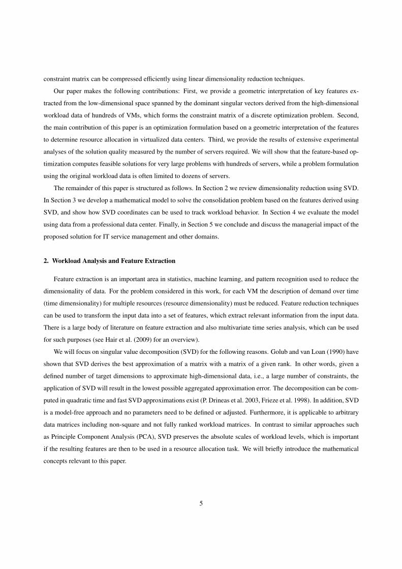
As an illustration how SVD works, consider workload r jl of items j in L = 2 dimensions (e.g., the maximum
workload demand for one resource K = 1 observed during daytimes (rl:=1) and nighttimes (rl:=2). Resulting data
points of item workloads are shown in Figure 1. For each j, coordinates (or features) u j1 in the first subspace, i.e.,
v 2
v1
r1
r 2
u11
item 1
u12
r12
r11
Figure 1: Item Workload Data Projections
along v1, the first right singular vector in VT , are calculated by perpendicular projection of the original points onto v1
6

as shown for item 1. These coordinates show the best one-dimensional approximation of the data because v1 captures
as much of data variation as possible in one direction. In other words, v1 is a regression line running through the
points in the direction where the data is most widely spread.
Item coordinates u j2 regarding the second right singular vector v2 (v2⊥v1) then capture the maximum variance
after removing the projections along v1. In this two-dimensional example, v2 captures all of the remaining variance.
In general, the number of singular vectors equals R’s rank.
Truncated SVD (tSVD) only considers the E dominant subspaces, i.e., the E row vectors of VT and the E column
vectors of U corresponding to the E largest singular values in Σ. Hence the rest of the matrix is discarded and the
original matrix R is approximated by∑E
e=1 ueσe(ve)T . The idea is that variation below a particular threshold E can be
ignored, if R’s effective rank does not exceed E (i.e., the rank corresponding to the E dominant singular values which
are ’significantly’ greater than zero), as the singular values associated with the right singular vectors sort them in the
order of the explained variation from most to least significant. Depending on the decay of singular values, very large
matrices can be approximated with high accuracy using only a very small set of singular vectors. Workload time series
of enterprise applications usually exhibit daily or weekly cycles and can be approximated well with only a small set
of subspaces. The resulting approximation errors are analyzed in the next subsection.
2.2. Matrix Norms and Approximation Errors
Let RE :=∑E
e=1 ueσe(ve)T be R’s approximation derived with the first E subspaces. Let then RεE := R − RE be
RE’s approximation error matrix (or residual matrix) with elements rεjl. Although the tSVD is no longer an exact
factorization of R, Eckart and Young (1936) have proven that RE is – in a useful sense for our purposes – the closest
approximation to R possible with a matrix of rank E taking the Frobenius norm || · ||F or the spectral norm || · ||2
(also known as matrix 2-norm) as a measure. Such matrix norms extend the concept of vector norms or distances to
matrices. They have shown that it is impossible to find a matrix A with rank E that satisfies (2).
||RεE ||F > ||R − A||F OR ||Rε
E ||2 > ||R − A||2 (2)
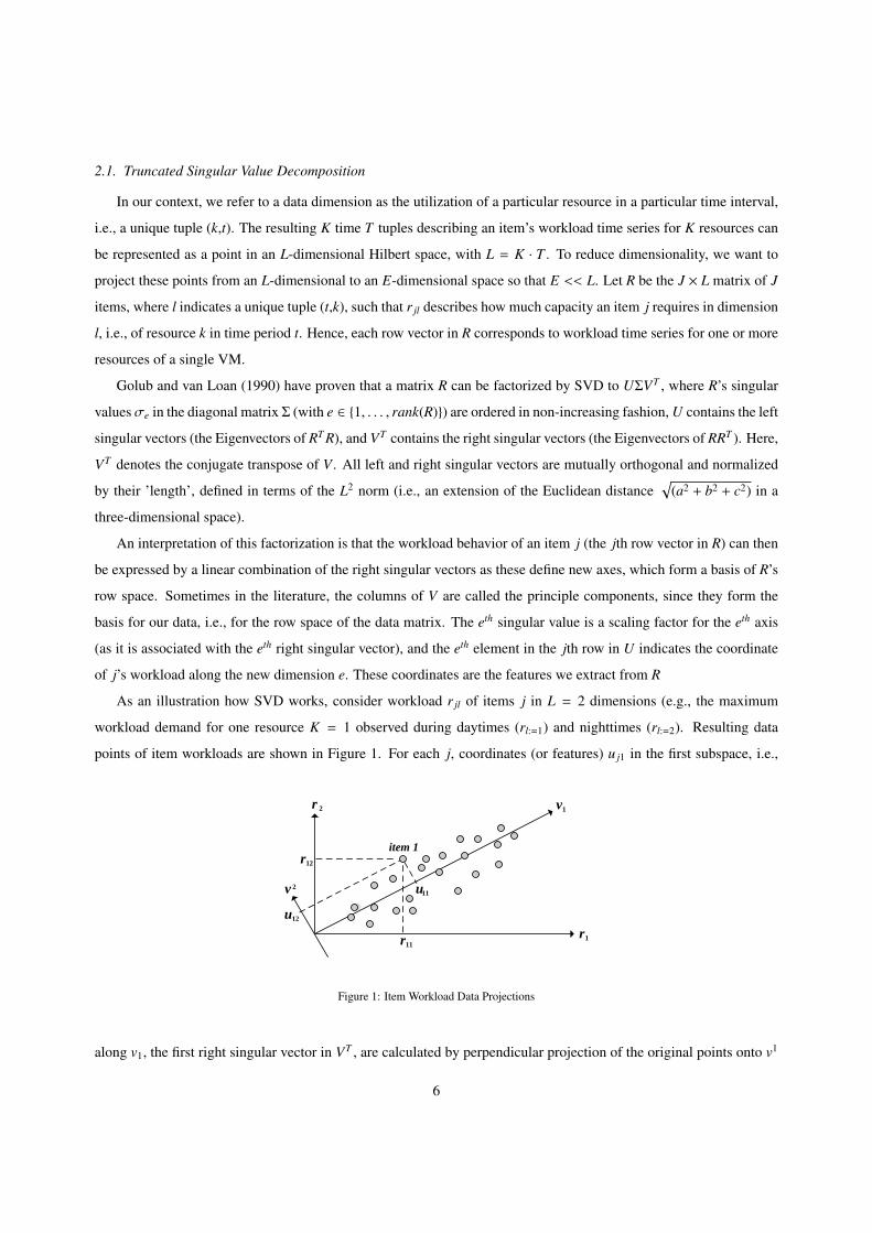
Consider the scenario depicted on the left-hand side of Figure 2. The graphs describe one-hour aggregates of
diurnal CPU workloads of 16 arbitrarily chosen enterprise applications taken from a data center log file from a large
European IT service provider. The underlying workload matrix R is of rank 16. Workload levels are described in
percent relative to the overall CPU performance of a server. The graph on the right-hand side of the figure shows the
reconstruction of the VM workload curves with E := 3, i.e., using the first three SVD subspaces. The graphs in Figure
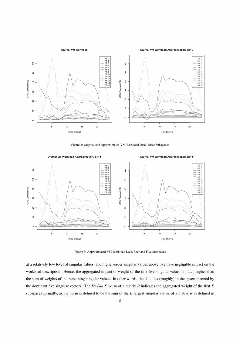
3 show the data reconstruction when using four and five subspaces, respectively. While the data approximation with
three SVD subspaces already yields the principal workload behavior, the approximation with five subspaces captures
the workload behavior, in particular for VM with higher workload that are of particular interest for our purposes,
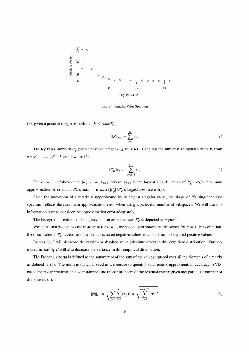
with high accuracy. The approximation works well due to the significant initial decay in R’s singular value spectrum
shown in Figure 4. The spectrum exhibits a sharp drop at the beginning and then continues with a moderate decay
7
Diurnal VM Workload
Time Interval
CP
U D
eman
d (%
)
5 10 15 20
010
2030
4050
60
VM 1VM 2VM 3VM 4VM 5VM 6VM 7VM 8VM 9VM 10VM 11VM 12VM 13VM 14VM 15VM 16
Diurnal VM Workload Approximation, E:= 3
Time Interval
CP
U D
eman
d (%
)
5 10 15 200
1020
3040
5060
VM 1VM 2VM 3VM 4VM 5VM 6VM 7VM 8VM 9VM 10VM 11VM 12VM 13VM 14VM 15VM 16
Figure 2: Original and Approximated VM Workload Data, Three Subspaces
Diurnal VM Workload Approximation, E:= 4
Time Interval
CP
U D
eman
d (%
)
5 10 15 20
010
2030
4050
60
VM 1VM 2VM 3VM 4VM 5VM 6VM 7VM 8VM 9VM 10VM 11VM 12VM 13VM 14VM 15VM 16
Diurnal VM Workload Approximation, E:= 5
Time Interval
CP
U D
eman
d (%
)
5 10 15 20
010
2030
4050
60
VM 1VM 2VM 3VM 4VM 5VM 6VM 7VM 8VM 9VM 10VM 11VM 12VM 13VM 14VM 15VM 16
Figure 3: Approximated VM Workload Data, Four and Five Subspaces
at a relatively low level of singular values, and higher-order singular values above five have negligible impact on the
workload description. Hence, the aggregated impact or weight of the first five singular values is much higher than
the sum of weights of the remaining singular values. In other words, the data lies (roughly) in the space spanned by
the dominant five singular vectors. The Ky Fan E norm of a matrix R indicates the aggregated weight of the first E
subspaces formally, as the norm is defined to be the sum of the E largest singular values of a matrix R as defined in
8
5 10 15
050
150
250
Singular Value Spectrum
Singular Value
Abs
olut
e W
eigh
t
Figure 4: Singular Value Spectrum
(3), given a positive integer E such that E ≤ rank(R).
||R||KE :=E∑
e=1
σe (3)
The Ky Fan F-norm of RεE (with a positive integer F ≤ rank(R)−E) equals the sum of R’s singular values σe from
e = E + 1, . . . , E + F as shown in (4).
||RεE ||KF :=
E+F∑e=E+1
σe (4)
For F := 1 it follows that ||RεE ||K1 = σE+1, where σE+1 is the largest singular value of Rε
E . RE’s maximum
approximation error equals RεE’s max-norm max j,l|rεjl| (R
εE’s largest absolute entry).
Since the max-norm of a matrix is upper-bound by its largest singular value, the shape of R’s singular value
spectrum reflects the maximum approximation error when using a particular number of subspaces. We will use this
information later to consider the approximation error adequately.
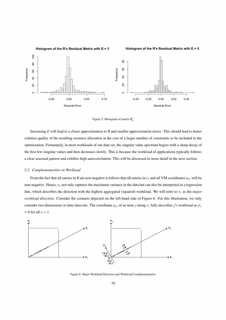
The histogram of entries in the approximation error matrices RεE is depicted in Figure 5.
While the first plot shows the histogram for E = 3, the second plot shows the histogram for E = 5. Per definition,
the mean value in RεE is zero, and the sum of squared negative values equals the sum of squared positive values.
Increasing E will decrease the maximum absolute value (absolute error) in this empirical distribution. Further-
more, increasing E will also decrease the variance in this empirical distribution.
The Frobenius norm is defined as the square root of the sum of the values squared over all the elements of a matrix
as defined in (5). The norm is typically used as a measure to quantify total matrix approximation accuracy. SVD-
based matrix approximation also minimizes the Frobenius norm of the residual matrix given any particular number of
dimensions (5).
||R||F :=
√√√ J∑j=1
L∑l=1
(r jl)2 =
√√√rank(R)∑e=1
(σe)2 (5)
9
Histogram of the R's Residual Matrix with E:= 3
Absolute Error
Frequency
-0.05 0.00 0.05 0.10
020
4060
80100
Histogram of the R's Residual Matrix with E:= 5
Absolute Error
Frequency
-0.04 -0.02 0.00 0.02 0.04
020
4060
80Figure 5: Histogram of matrix RεE
Increasing E will lead to a closer approximation to R and smaller approximation errors. This should lead to better
solution quality of the resulting resource allocation at the cost of a larger number of constraints to be included in the
optimization. Fortunately, in most workloads of our data set, the singular value spectrum begins with a sharp decay of
the first few singular values and then decreases slowly. This is because the workload of applications typically follows
a clear seasonal pattern and exhibits high autocorrelation. This will be discussed in more detail in the next section.
2.3. Complementarities in Workload
From the fact that all entries in R are non-negative it follows that all entries in v1 and all VM coordinates u j1 will be
non-negative. Hence, v1 not only captures the maximum variance in the data but can also be interpreted as a regression
line, which describes the direction with the highest aggregated (squared) workload. We will refer to v1 as the major
workload direction. Consider the scenario depicted on the left-hand side of Figure 6. For this illustration, we only
consider two dimensions or time intervals. The coordinate u j1 of an item j along v1 fully describes j’s workload as σe
= 0 for all e > 1.
v1
r 1
r2
v2 ab
cd+0.2
+0.1-0.2-0.1
0
r 2
r1
v1
Figure 6: Major Workload Direction and Workload Complementarities
10
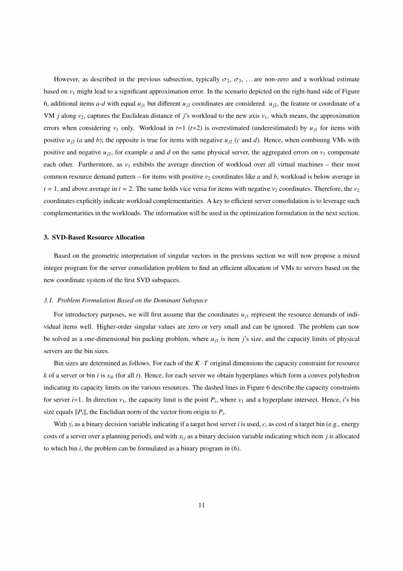
However, as described in the previous subsection, typically σ2, σ3, . . . are non-zero and a workload estimate
based on v1 might lead to a significant approximation error. In the scenario depicted on the right-hand side of Figure
6, additional items a-d with equal u j1 but different u j2 coordinates are considered. u j2, the feature or coordinate of a
VM j along v2, captures the Euclidean distance of j’s workload to the new axis v1, which means, the approximation
errors when considering v1 only. Workload in t=1 (t=2) is overestimated (underestimated) by u j1 for items with
positive u j2 (a and b); the opposite is true for items with negative u j2 (c and d). Hence, when combining VMs with
positive and negative u j2, for example a and d on the same physical server, the aggregated errors on v1 compensate
each other. Furthermore, as v1 exhibits the average direction of workload over all virtual machines – their most
common resource demand pattern – for items with positive v2 coordinates like a and b, workload is below average in
t = 1, and above average in t = 2. The same holds vice versa for items with negative v2 coordinates. Therefore, the v2
coordinates explicitly indicate workload complementarities. A key to efficient server consolidation is to leverage such
complementarities in the workloads. The information will be used in the optimization formulation in the next section.
3. SVD-Based Resource Allocation
Based on the geometric interpretation of singular vectors in the previous section we will now propose a mixed
integer program for the server consolidation problem to find an efficient allocation of VMs to servers based on the
new coordinate system of the first SVD subspaces.
3.1. Problem Formulation Based on the Dominant Subspace
For introductory purposes, we will first assume that the coordinates u j1 represent the resource demands of indi-
vidual items well. Higher-order singular values are zero or very small and can be ignored. The problem can now
be solved as a one-dimensional bin packing problem, where u j1 is item j’s size, and the capacity limits of physical
servers are the bin sizes.
Bin sizes are determined as follows. For each of the K · T original dimensions the capacity constraint for resource
k of a server or bin i is sik (for all t). Hence, for each server we obtain hyperplanes which form a convex polyhedron
indicating its capacity limits on the various resources. The dashed lines in Figure 6 describe the capacity constraints
for server i=1. In direction v1, the capacity limit is the point Pi, where v1 and a hyperplane intersect. Hence, i’s bin
size equals ||Pi||, the Euclidian norm of the vector from origin to Pi.
With yi as a binary decision variable indicating if a target host server i is used, ci as cost of a target bin (e.g., energy
costs of a server over a planning period), and with xi j as a binary decision variable indicating which item j is allocated
to which bin i, the problem can be formulated as a binary program in (6).
11
min∑i
ci · yi
s.t.∑i≤I
xi j = 1 ∀ j ≤ J∑j≤J
u1j · xi j ≤ ||Pi||yi ∀i ≤ I
yi, xi j ∈ {0, 1} ∀i ≤ I,∀ j ≤ J
(6)
The objective is to minimize total costs and the first constraint ensures that each item is allocated exactly once. The
second constraint ensures that the aggregated v1-based workload estimate of items assigned to a bin does not exceed
the bin’s capacity limit.
3.2. Consideration of Higher-Order Subspaces
Typically, higher-order singular values of R are non-zero and one needs to take into account the deviations from
the workload estimates in dimension v1. Let us first focus on E = 2 as v2 is the major direction of the deviation from
v1. Higher dimensions of E > 2 can then be handled analogously.
In order to avoid overload situations, u j2, the deviations from v1 need to be added to the v1 coordinates of each item.
As we have seen in Section 2.3, positive and negative coordinates u j2 describe complementarities in the workload.
Combining only items with positive u j2 in a bin increases the approximation error from v1, while the opposite is the
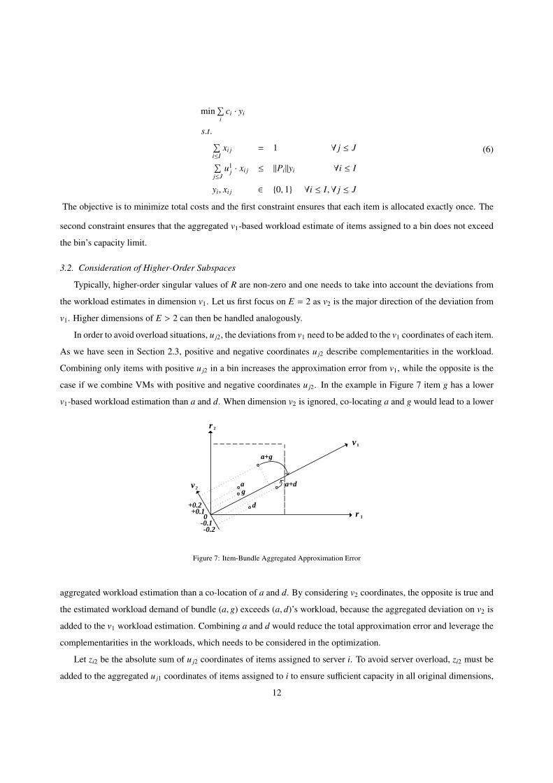
case if we combine VMs with positive and negative coordinates u j2. In the example in Figure 7 item g has a lower
v1-based workload estimation than a and d. When dimension v2 is ignored, co-locating a and g would lead to a lower
v1
r 1
r 2
v2ag
d+0.2+0.1
-0.2
0
a+d
a+g
-0.1
Figure 7: Item-Bundle Aggregated Approximation Error
aggregated workload estimation than a co-location of a and d. By considering v2 coordinates, the opposite is true and
the estimated workload demand of bundle (a, g) exceeds (a, d)’s workload, because the aggregated deviation on v2 is
added to the v1 workload estimation. Combining a and d would reduce the total approximation error and leverage the
complementarities in the workloads, which needs to be considered in the optimization.
Let zi2 be the absolute sum of u j2 coordinates of items assigned to server i. To avoid server overload, zi2 must be
added to the aggregated u j1 coordinates of items assigned to i to ensure sufficient capacity in all original dimensions,
12
i.e., for all time intervals and for all resources. The resulting program considering deviations from v1 is shown in (7),
where we assign variables for positive and negative zi2.
min∑i
ci · yi
s.t.∑i≤I
xi j = 1 ∀ j ≤ J∑j≤J
(u j2 · xi j) − z+i2 + z−i2 = 0 ∀i ≤ I∑
j≤J(u j1 · xi j) + z+
i2 + z−i2 ≤ ||Pi||yi ∀i ≤ I
yi, xi j ∈ {0, 1} ∀i ≤ I,∀ j ≤ J
z+i2, z
−i2 ≥ 0 ∀i ≤ I
(7)
We will refer to this problem formulation in (7) as SVD-based packing or SVPack. Again, the objective is to
minimize server costs and the first constraint ensures that each VM is allocated exactly once. The second constraint
determines z+i2 and z−i2, which are either positive or negative deviations on v2 required in the third constraint. The third
constraint ensures that the aggregated v1-based workload estimate of VMs assigned to a target plus the deviations z+i2
and z−i2 do not exceed the target’s capacity limit. Variations along v3, v4, . . . can be considered similar to those in v2,
if the respective singular values are significant. For each e {2 <e <E} and each server i we introduce a constraint to
determine z+ie and z−ie and add those variables to the left-hand side of the third constraint type in (7). The number of
constraints in SVPack grows with O(EJ), the number of decision variables with O(JI + I). Section ?? and Section 4.3
provide a detailed analysis of the number of variables and constraints in MBP and SVPack.
3.3. Workload Analysis and Visualization
SVD provides a powerful method to extract relevant features from large data sets. While the main focus of this
paper is on server consolidation, we also want to discuss applications of SVD to derive metrics that can support
management decisions. Here, we will focus on the monitoring of relevant workload characteristics over time.
Server consolidation aims at finding an efficient allocation of VMs to servers, such that reallocations are unneces-
sary, if workload patterns do not change. In virtualized data centers, some VMs are withdrawn over time, while new
ones need to be deployed. Also, workload patterns can change over time. For example, a VM hosting an e-commerce
application might face increased workload around Christmas. In order to avoid overload situations, a controller needs
to monitor workload developments and migrate VMs before the overall workload on a physical server hits the server’s
capacity bounds.
However, migrations cause significant CPU and network bandwidth overheads and must be triggered early, before
a system’s workload becomes too high. During the duration of a migration, additional CPU cycles up to 70% of the
actual CPU demand of a VM are required, and the network bandwidth usage can saturate even a 1 GB/s network link
for minutes to transfer the memory of a VM from one server to another. The CPU overhead is mainly due to additional
13
I/O operations for main memory transfer from the source to the target server and the memory management via shadow
pages.
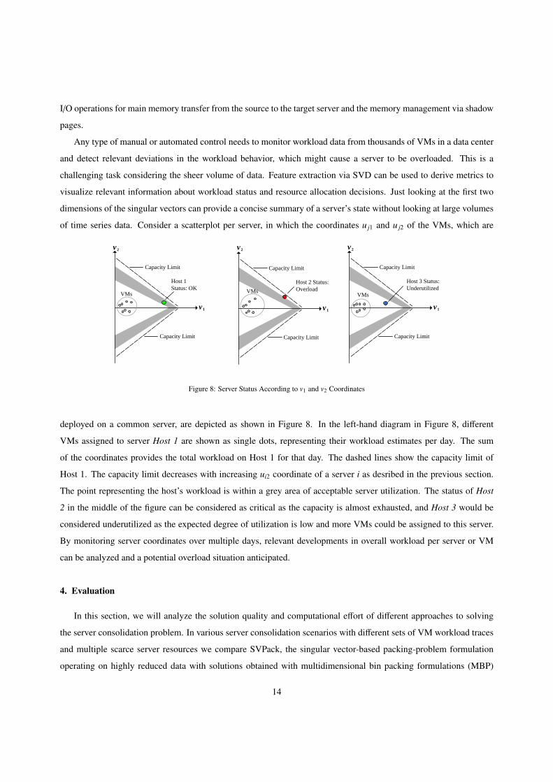
Any type of manual or automated control needs to monitor workload data from thousands of VMs in a data center
and detect relevant deviations in the workload behavior, which might cause a server to be overloaded. This is a
challenging task considering the sheer volume of data. Feature extraction via SVD can be used to derive metrics to
visualize relevant information about workload status and resource allocation decisions. Just looking at the first two
dimensions of the singular vectors can provide a concise summary of a server’s state without looking at large volumes
of time series data. Consider a scatterplot per server, in which the coordinates u j1 and u j2 of the VMs, which are
v 1
v 2
VMs
Host 1 Status: OK
Capacity Limit
Capacity Limit
v 1
VMsHost 2 Status: Overload
Capacity Limit
Capacity Limit
v1
VMs
Host 3 Status: Underutilized
Capacity Limit
Capacity Limit
v2 v 2
Figure 8: Server Status According to v1 and v2 Coordinates
deployed on a common server, are depicted as shown in Figure 8. In the left-hand diagram in Figure 8, different
VMs assigned to server Host 1 are shown as single dots, representing their workload estimates per day. The sum
of the coordinates provides the total workload on Host 1 for that day. The dashed lines show the capacity limit of
Host 1. The capacity limit decreases with increasing ui2 coordinate of a server i as desribed in the previous section.
The point representing the host’s workload is within a grey area of acceptable server utilization. The status of Host
2 in the middle of the figure can be considered as critical as the capacity is almost exhausted, and Host 3 would be
considered underutilized as the expected degree of utilization is low and more VMs could be assigned to this server.
By monitoring server coordinates over multiple days, relevant developments in overall workload per server or VM
can be analyzed and a potential overload situation anticipated.
4. Evaluation
In this section, we will analyze the solution quality and computational effort of different approaches to solving
the server consolidation problem. In various server consolidation scenarios with different sets of VM workload traces
and multiple scarce server resources we compare SVPack, the singular vector-based packing-problem formulation
operating on highly reduced data with solutions obtained with multidimensional bin packing formulations (MBP)
14
operating on different aggregation levels of the original workload data. We will take the number of servers required
to host a set of VMs in a certain scenario as a metric for solution quality. First, we describe the available data set and
the research design, before discussing the main results.
4.1. Data and Component Day Extraction
The workload data provided by a large European data center operator describes the CPU, I/O, and main memory
usage monitored in intervals of five minutes over ten consecutive weeks for 458 enterprise applications. The applica-
tions stem from a diverse set of customers in various industries and include Web servers, application servers, database
servers, and ERP applications.
Similar to Parent (2005), we found that a majority of the business applications hosted in data centers exhibit
quite regular and cyclic workload patterns. As mentioned above, regular, periodic patterns in workload data can
be leveraged in server consolidation, where the selection of VMs with complementary workload traces allows the
multiplexing of resources over time and the utilizing of resources more efficiently.
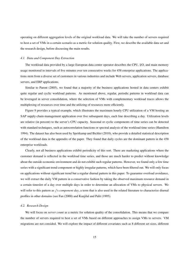
Figure 9 provides a typical example, which illustrates the maximum hourly CPU utilization of a VM hosting an
SAP supply-chain-management application over five subsequent days, each line describing a day. Utilization levels
are relative (in percent) to the server’s CPU capacity. Seasonal or cyclic components of time series can be detected
with standard techniques, such as autocorrelation functions or spectral analysis of the workload time series (Hamilton
1994). The dataset has also been used by Speitkamp and Bichler (2010), who provide a detailed statistical description
of the workload data in the appendix of the paper. They found that daily cycles are the dominant pattern in the 458
enterprise workloads.
Clearly, not all business applications exhibit periodicity of this sort. There are marketing applications where the
customer demand is reflected in the workload time series, and those are much harder to predict without knowledge
about the outside economic environment and do not exhibit such regular patterns. However, we found only a few time
series with a significant trend component or highly irregular patterns, which have been filtered out. We will only focus
on applications without significant trend but a regular diurnal pattern in this paper. To guarantee overload avoidance,
we will extract the daily VM pattern in a conservative fashion by taking the observed maximum resource demand in
a certain timeslot of a day over multiple days in order to determine an allocation of VMs to physical servers. We
will refer to this pattern as j’s component day, a term that is also used in the related literature to characterize diurnal
profiles in other domains (see Fan (2000) and Kanjilal and Palit (1995).
4.2. Research Design
We will focus on server count as a metric for solution quality of the consolidation. This means that we compare
the number of servers required to host a set of VMs based on different approaches to assign VMs to servers. VM
migrations are not consided. We will explore the impact of different covariates such as 8 different set sizes, different
15
Workload Profile over Five Days, VM 5
Time (hour)
Util
izat
ion
Leve
l (C
PU
)
5 10 15 20
05
1015
2025
30
Utilization, Day 1Utilization, Day 2Utilization, Day 3Utilization, Day 4Utilization, Day 5
Figure 9: Daily workload traces of an ERP application
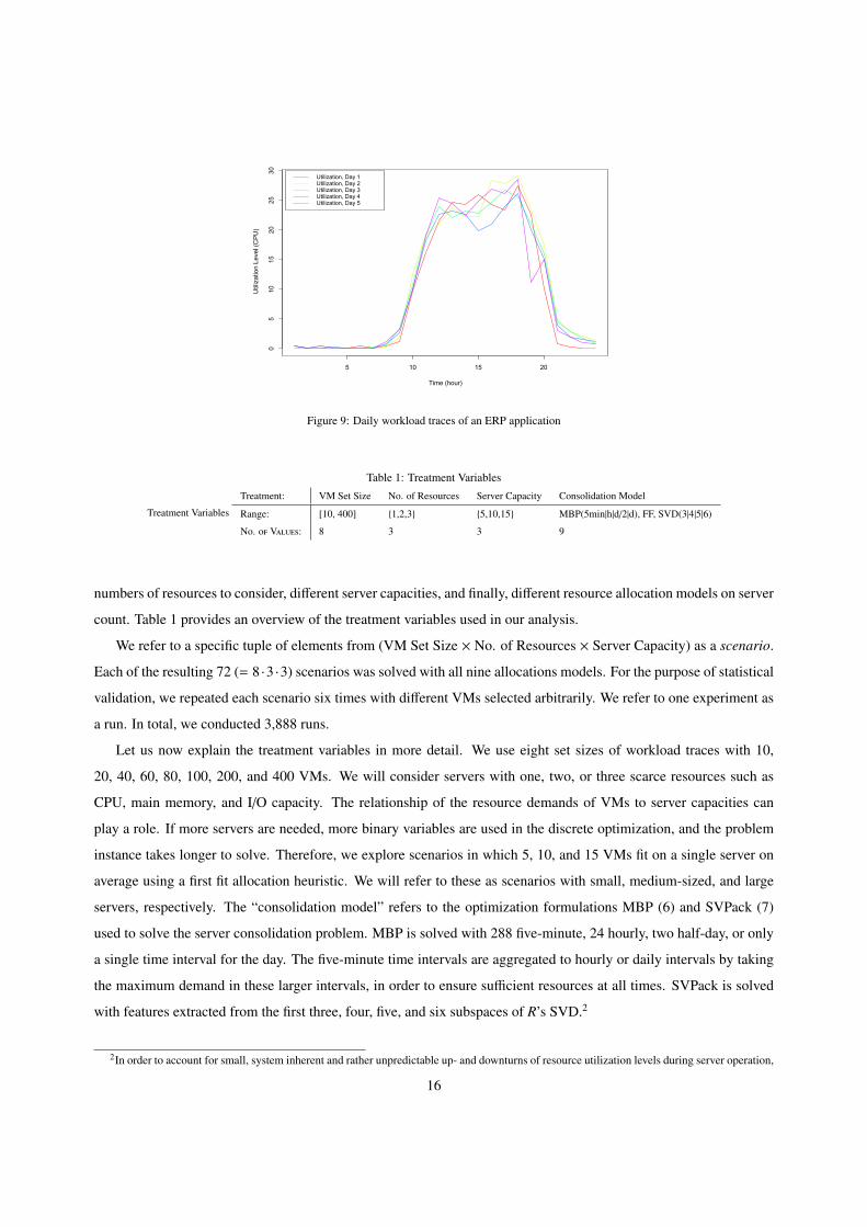
Table 1: Treatment Variables
Treatment Variables
Treatment: VM Set Size No. of Resources Server Capacity Consolidation Model
Range: [10, 400] {1,2,3} {5,10,15} MBP(5min|h|d/2|d), FF, SVD(3|4|5|6)
No. of Values: 8 3 3 9
numbers of resources to consider, different server capacities, and finally, different resource allocation models on server
count. Table 1 provides an overview of the treatment variables used in our analysis.
We refer to a specific tuple of elements from (VM Set Size × No. of Resources × Server Capacity) as a scenario.
Each of the resulting 72 (= 8 ·3 ·3) scenarios was solved with all nine allocations models. For the purpose of statistical
validation, we repeated each scenario six times with different VMs selected arbitrarily. We refer to one experiment as
a run. In total, we conducted 3,888 runs.
Let us now explain the treatment variables in more detail. We use eight set sizes of workload traces with 10,
20, 40, 60, 80, 100, 200, and 400 VMs. We will consider servers with one, two, or three scarce resources such as
CPU, main memory, and I/O capacity. The relationship of the resource demands of VMs to server capacities can
play a role. If more servers are needed, more binary variables are used in the discrete optimization, and the problem
instance takes longer to solve. Therefore, we explore scenarios in which 5, 10, and 15 VMs fit on a single server on
average using a first fit allocation heuristic. We will refer to these as scenarios with small, medium-sized, and large
servers, respectively. The “consolidation model” refers to the optimization formulations MBP (6) and SVPack (7)
used to solve the server consolidation problem. MBP is solved with 288 five-minute, 24 hourly, two half-day, or only
a single time interval for the day. The five-minute time intervals are aggregated to hourly or daily intervals by taking
the maximum demand in these larger intervals, in order to ensure sufficient resources at all times. SVPack is solved
with features extracted from the first three, four, five, and six subspaces of R’s SVD.2
2In order to account for small, system inherent and rather unpredictable up- and downturns of resource utilization levels during server operation,
16
We have also implemented a simple multidimensional first fit heuristic (FF), which stacks one VM on top of
the other until the capacity in one dimension is violated. Such heuristics do not consider side constraints and are
therefore not applicable in most practical settings, but the results help us evaluate the solution quality of branch-and-
cut algorithms in our experiments, which could not be solved to optimality.
All calculations are performed on a 2.4 Ghz Intel Duo with 4GB RAM using R for SVD calculation and IBM
ILOG CPLEX 12.2 as the branch-and-cut solver. MBP with five-minute time intervals MBP(5min) serves as a lower
bound for all other allocations, as this formulation uses all available data. No formulation which operates on reduced
data can lead to a better solution. However, even for MBP(5min) with only 40 or 60 VMs and two or three resources
the computation time for many problem instances exceeds days. For larger problems with a few hundred VMs we
could not even find a feasible solution that improves a FF solution with MDP(5min) because of the huge main memory
requirements to store intermediate node-sets, which finally caused the solver to abort processing.
We will therefore use the objective function value of the LP relaxation of the MBP(5min) formulation (6) as a
lower bound. In other words, we will assume that we can assign also parts of a VM on different physical servers. This
allocation is technically not feasible, but easy to calculate and serves as a convenient lower bound for any feasible
allocation considering that an entire VM needs to be hosted on a physical server.
Consultants typically want to analyze consolidation problems with different side constraints and different selec-
tions of VMs when working with a customer. Such problems need to be solved within a much smaller timeframe.
MIP solvers allow the termination of the processing after a certain time limit and return the best integer solution found
so far. The difference between the best LP relaxation in the branch-and-bound tree and the best integer solution found
can serve as a worst-case estimate for optimality of the allocation. We found that even for large problems with 200 or
400 VMs, typically a feasible solution found within 30 minutes could not or could only marginally be improved after
a computation time of a day or even a week. So, we have used a time limit of 30 minutes for each problem and used
the best integer solution found. Note that the time to compute the SVD of R never exceeded ten seconds, even for the
largest instances.
4.3. Results
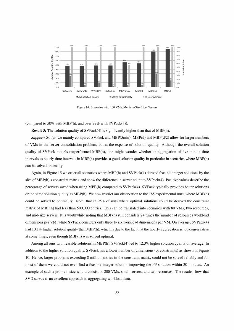
Aggregated results of our experiments are shown in Figure 10. For each consolidation model, the first (left)
two bars are associated with the primary (left) Y-axis of the diagram and show the average solution quality of the
consolidation model and the standard deviation of this solution quality. Again, solution quality was measured in
number of servers required in the allocation relative to the objective function value of the LP relaxation of MBP(5min).
IT service managers can parameterize the right-hand side vectors of the models with slightly lower capacity constraints learned from workload
history, leaving a safety resource buffer to avoid unplanned overload situations. In other words, the consolidation models are parameterized with
the remaining resource capacity set to 100% without changing the structure of the models. In this work we exclude the computation of safety
buffers and focus on the efficiency of consolidation models.
17
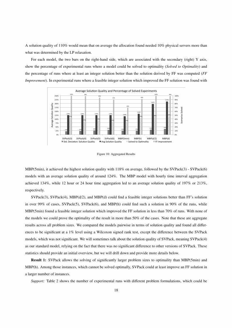
A solution quality of 110% would mean that on average the allocation found needed 10% physical servers more than
what was determined by the LP relaxation.
For each model, the two bars on the right-hand side, which are associated with the secondary (right) Y axis,
show the percentage of experimental runs where a model could be solved to optimality (Solved to Optimality) and
the percentage of runs where at least an integer solution better than the solution derived by FF was computed (FF
Improvement). In experimental runs where a feasible integer solution which improved the FF solution was found with
21% 23% 26% 30%24% 25%
31% 35%
124% 124% 124% 124%118%
134%
197%
213%
43%
34%36%
33% 32%
43% 45%47%
100% 99%95%
91%
69%
92%
100% 99%
0%
10%
20%
30%
40%
50%
60%
70%
80%
90%
100%
0%
25%
50%
75%
100%
125%
150%
175%
200%
225%
250%
SVPack(3) SVPack(4) SVPack(5) SVPack(6) MBP(5min) MBP(h) MBP(d/2) MBP(d)
Scen
ariosSolved
AverageSoluFo
nQuality
AverageSoluFonQualityandPercentageofSolvedExperiments
Std.DeviaFon:SoluFonQuality AvgSoluFonQuality SolvedtoOpFmality FFImprovement
Figure 10: Aggregated Results
MBP(5min), it achieved the highest solution quality with 118% on average, followed by the SVPack(3) - SVPack(6)
models with an average solution quality of around 124%. The MBP model with hourly time interval aggregation
achieved 134%, while 12 hour or 24 hour time aggregation led to an average solution quality of 197% or 213%,
respectively.
SVPack(3), SVPack(4), MBP(d/2), and MBP(d) could find a feasible integer solutions better than FF’s solution
in over 99% of cases, SVPack(5), SVPack(6), and MBP(h) could find such a solution in 90% of the runs, while
MBP(5min) found a feasible integer solution which improved the FF solution in less than 70% of runs. With none of
the models we could prove the optimality of the result in more than 50% of the cases. Note that these are aggregate
results across all problem sizes. We compared the models pairwise in terms of solution quality and found all differ-
ences to be significant at a 1% level using a Wilcoxon signed rank test, except the difference between the SVPack
models, which was not significant. We will sometimes talk about the solution quality of SVPack, meaning SVPack(4)
as our standard model, relying on the fact that there was no significant difference to other versions of SVPack. These
statistics should provide an initial overview, but we will drill down and provide more details below.
Result 1: SVPack allows the solving of significantly larger problem sizes to optimality than MBP(5min) and
MBP(h). Among those instances, which cannot be solved optimally, SVPack could at least improve an FF solution in
a larger number of instances.
Support: Table 2 shows the number of experimental runs with different problem formulations, which could be
18
solved to optimality (Optimal), where no optimal, but a feasible equal or better than the FF solution could be found
(Feasible), and where no feasible solution could be found which was at least as good as an FF solution (No Solution)
grouped by VM set size and server size, the two key drivers for the size of an underlying constraint matrix.
With MBP(5min), no scenario with more than 40 VMs could be solved to optimality. In scenarios with small host
servers, we could not compute an optimal solution even in scenarios with only 20 VMs and three resources within 30
minutes in two-thirds of the runs. Furthermore, in such scenarios with small servers and VM set sizes of 100 or more,
no feasible integer solution equal or better than FF could be found at all with MBP(5min).
In MBP(h) problems with up to 100 VMs could be solved to optimality, and for problems with fewer than 200
servers at least feasible integer solutions which improved the FF solutions were found. In scenarios with small host
servers, solutions are found for VM set sizes up to 100. With MBP(d) and SVPack(4) we found feasible solutions for
all scenarios. Only in two runs with small servers and 400 VMs could MBP(d) not find a feasible solution. Also, in
two out of six runs we could find no feasible integer solution with SVPack(4), in scenarios with 400 VMs and small
or medium-sized servers.
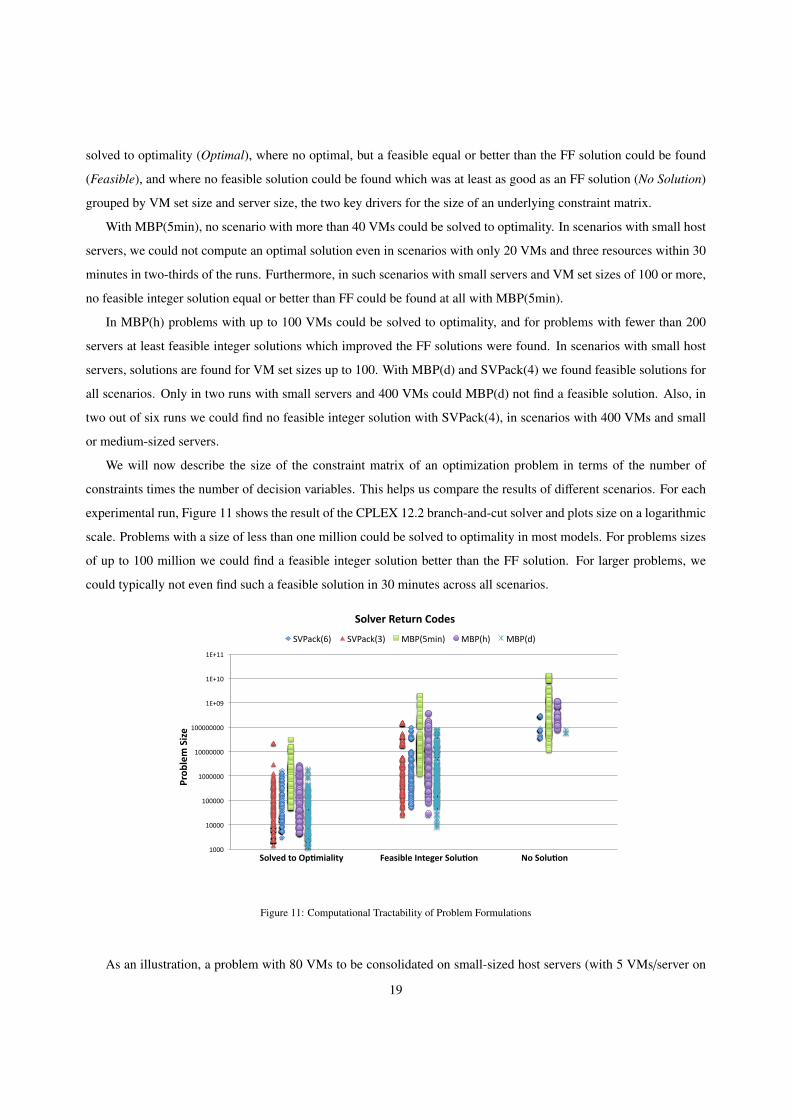
We will now describe the size of the constraint matrix of an optimization problem in terms of the number of
constraints times the number of decision variables. This helps us compare the results of different scenarios. For each
experimental run, Figure 11 shows the result of the CPLEX 12.2 branch-and-cut solver and plots size on a logarithmic
scale. Problems with a size of less than one million could be solved to optimality in most models. For problems sizes
of up to 100 million we could find a feasible integer solution better than the FF solution. For larger problems, we
could typically not even find such a feasible solution in 30 minutes across all scenarios.
1000
10000
100000
1000000
10000000
100000000
1E+09
1E+10
1E+11
Prob
lem Size
Solved to Op1miality Feasible Integer Solu1on No Solu1on
Solver Return Codes
SVPack(6) SVPack(3) MBP(5min) MBP(h) MBP(d)
Figure 11: Computational Tractability of Problem Formulations
As an illustration, a problem with 80 VMs to be consolidated on small-sized host servers (with 5 VMs/server on
19
average), with two resource types under consideration, leads to the following problem sizes shown in Table 3.
With an MBP(5min) formulation with a problem size of 12 million, the problem is already such that it can not
be solved to optimality and mostly not even feasible solutions can be found. Besides its computational complexity,
the allocated memory in scenarios with 200 VMs exceeded 80 Gigabyte main memory with MBP(5min). With four
Gigabyte main memory available, the CPU was waiting more than 99% of the time for data swapped between main
memory and harddisk before the solver finally aborted the computation. In contrast, if SVPack(3) or SVPack(4) is
used, the very same problem can be solved to optimality. Even in the largest scenario with 400 VMs and small host
servers the solver could at least find an integer solution for the S VPack(3) formulation that required fewer or equal
servers than the solution derived with FF in all but four runs in 30 minutes.
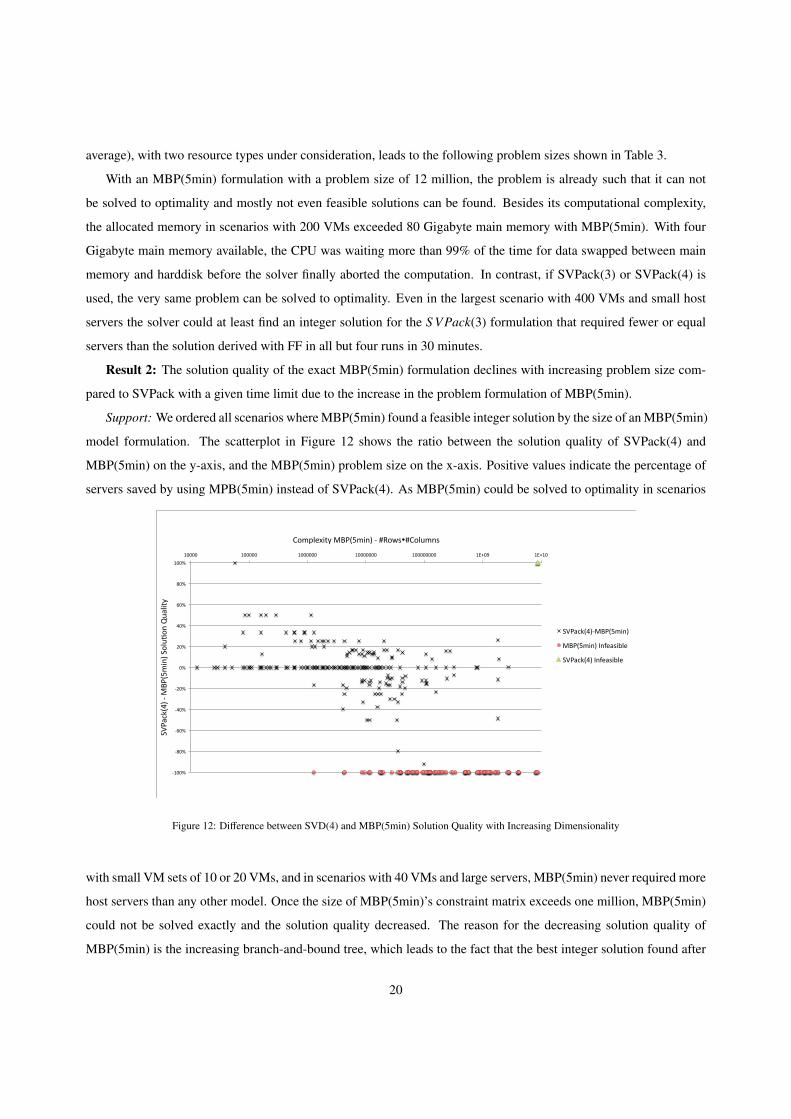
Result 2: The solution quality of the exact MBP(5min) formulation declines with increasing problem size com-
pared to SVPack with a given time limit due to the increase in the problem formulation of MBP(5min).
Support: We ordered all scenarios where MBP(5min) found a feasible integer solution by the size of an MBP(5min)
model formulation. The scatterplot in Figure 12 shows the ratio between the solution quality of SVPack(4) and
MBP(5min) on the y-axis, and the MBP(5min) problem size on the x-axis. Positive values indicate the percentage of
servers saved by using MPB(5min) instead of SVPack(4). As MBP(5min) could be solved to optimality in scenarios
-‐100%
-‐80%
-‐60%
-‐40%
-‐20%
0%
20%
40%
60%
80%
100%
10000 100000 1000000 10000000 100000000 1E+09 1E+10
SVPack(4) -‐ M
BP(5min) Solu>
on Quality
Complexity MBP(5min) -‐ #Rows#Columns
SVPack(4)-‐MBP(5min)
MBP(5min) Infeasible
SVPack(4) Infeasible
Figure 12: Difference between SVD(4) and MBP(5min) Solution Quality with Increasing Dimensionality
with small VM sets of 10 or 20 VMs, and in scenarios with 40 VMs and large servers, MBP(5min) never required more
host servers than any other model. Once the size of MBP(5min)’s constraint matrix exceeds one million, MBP(5min)
could not be solved exactly and the solution quality decreased. The reason for the decreasing solution quality of
MBP(5min) is the increasing branch-and-bound tree, which leads to the fact that the best integer solution found after
20
30 minutes is typically much worse than the optimal solution. Note that with MBP(5min), even problems with 60
VMs, two resource, and mid-size host servers, or problems with 40 VMs, small servers and three resources led to a
constraint matrix with more than 1.3 million entries. It is also important to note that we ignored the major portion
of runs with larger problems where no feasible integer solution could be found with MPB(5min) in Figure 12 (these
instances are marked red).
Even in small scenarios with less than one million entries in the constraint matrix of MBP(5min), SVPack achieved
the some solution quality as MBP(5min) in the majority of runs. On average, in small scenarios with a constraint
matrix of less than four million entries in MBP(5min) the solution quality of SVPack(4) was 7.8% worse. In scenarios
with MBP(5min) problem sizes between four million and 15 million entries, there was no significant difference in the
solution quality (Wilcoxon rank test, p = 0.7292). In scenarios exceeding 15 million entries, MBP(5min) only found
a feasible solution in less than 40% of the runs.
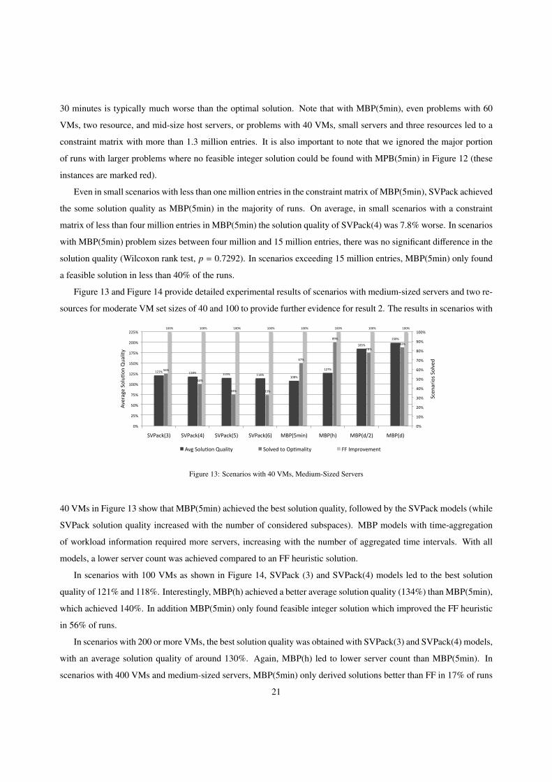
Figure 13 and Figure 14 provide detailed experimental results of scenarios with medium-sized servers and two re-
sources for moderate VM set sizes of 40 and 100 to provide further evidence for result 2. The results in scenarios with
121% 118% 115% 114%108%
127%
185%
199%
56%
44%
33% 33%
67%
89%
78%
83%
100% 100% 100% 100% 100% 100% 100% 100%
0%
10%
20%
30%
40%
50%
60%
70%
80%
90%
100%
0%
25%
50%
75%
100%
125%
150%
175%
200%
225%
SVPack(3) SVPack(4) SVPack(5) SVPack(6) MBP(5min) MBP(h) MBP(d/2) MBP(d)Scen
ariosSolved
AverageSoluFo
nQuality
AverageSoluFonQualityandNumberofSolvedExperiments40VMs,Medium‐SizedServers
AvgSoluFonQuality SolvedtoOpFmality FFImprovement
Figure 13: Scenarios with 40 VMs, Medium-Sized Servers
40 VMs in Figure 13 show that MBP(5min) achieved the best solution quality, followed by the SVPack models (while
SVPack solution quality increased with the number of considered subspaces). MBP models with time-aggregation
of workload information required more servers, increasing with the number of aggregated time intervals. With all
models, a lower server count was achieved compared to an FF heuristic solution.
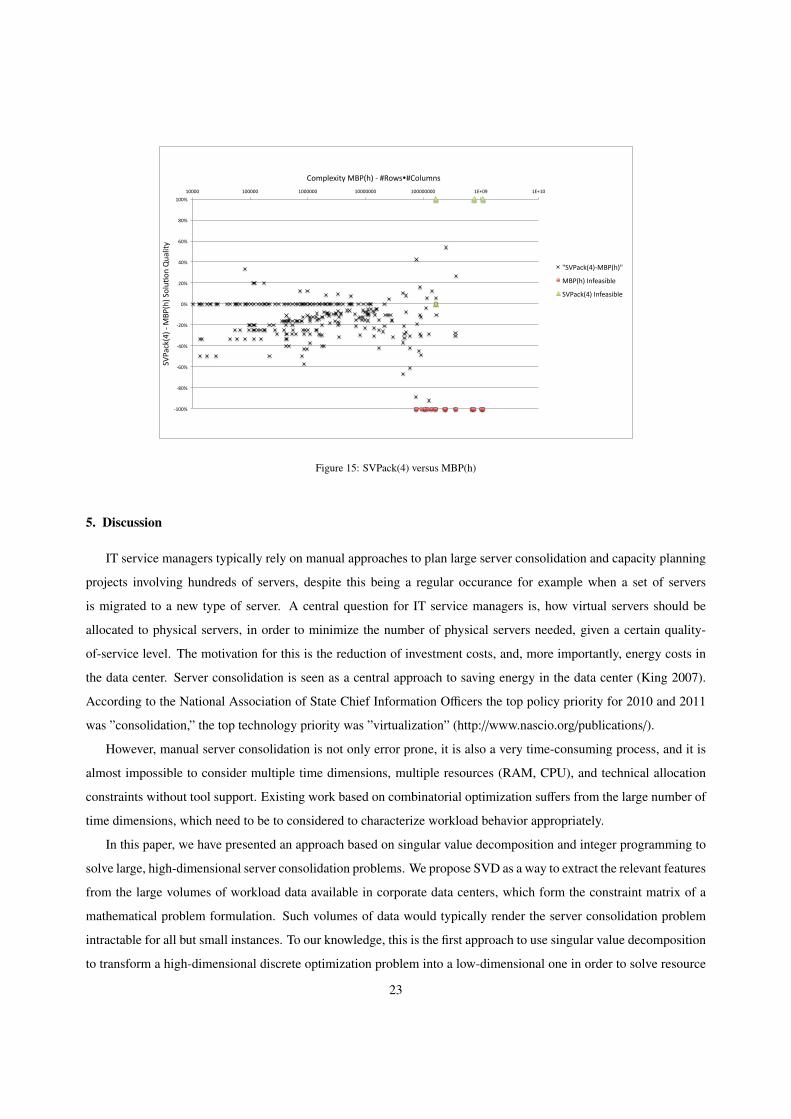
In scenarios with 100 VMs as shown in Figure 14, SVPack (3) and SVPack(4) models led to the best solution
quality of 121% and 118%. Interestingly, MBP(h) achieved a better average solution quality (134%) than MBP(5min),
which achieved 140%. In addition MBP(5min) only found feasible integer solution which improved the FF heuristic
in 56% of runs.
In scenarios with 200 or more VMs, the best solution quality was obtained with SVPack(3) and SVPack(4) models,
with an average solution quality of around 130%. Again, MBP(h) led to lower server count than MBP(5min). In
scenarios with 400 VMs and medium-sized servers, MBP(5min) only derived solutions better than FF in 17% of runs
21
121% 118% 122% 122%
140%134%
201%
216%
28%
6%
11%
3%6% 6%
33%
17%
100% 100% 100% 100%
56%
100% 100% 100%
0%
10%
20%
30%
40%
50%
60%
70%
80%
90%
100%
0%
25%
50%
75%
100%
125%
150%
175%
200%
225%
SVPack(3) SVPack(4) SVPack(5) SVPack(6) MBP(5min) MBP(h) MBP(d/2) MBP(d)
Scen
ariosSolved
AverageSoluFo
nQuality
AverageSoluFonQualityandNumberofSolvedExperiments100VMs,Medium‐SizedServers
AvgSoluFonQuality SolvedtoOpFmality FFImprovement
Figure 14: Scenarios with 100 VMs, Medium-Size Host Servers
(compared to 50% with MBP(h), and over 99% with SVPack(3)).
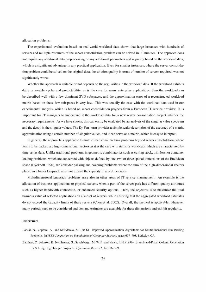
Result 3: The solution quality of SVPack(4) is significantly higher than that of MBP(h).
Support: So far, we mainly compared SVPack and MBP(5min). MBP(d) and MBP(d/2) allow for larger numbers
of VMs in the server consolidation problem, but at the expense of solution quality. Although the overall solution
quality of SVPack models outperformed MBP(h), one might wonder whether an aggregation of five-minute time
intervals to hourly time intervals in MBP(h) provides a good solution quality in particular in scenarios where MBP(h)
can be solved optimally.
Again, in Figure 15 we order all scenarios where MBP(h) and SVPack(4) derived feasible integer solutions by the
size of MBP(h)’s constraint matrix and show the difference in server count to SVPack(4). Positive values describe the
percentage of servers saved when using MPB(h) compared to SVPack(4). SVPack typically provides better solutions
or the same solution quality as MBP(h). We now restrict our observation to the 185 experimental runs, where MBP(h)
could be solved to optimality. Note, that in 95% of runs where optimal solutions could be derived the constraint
matrix of MBP(h) had less than 500,000 entries. This can be translated into scenarios with 80 VMs, two resources,
and mid-size servers. It is worthwhile noting that MBP(h) still considers 24 times the number of resources workload
dimensions per VM, while SVPack considers only three to six workload dimensions per VM. On average, SVPack(4)
had 10.1% higher solution quality than MBP(h), which is due to the fact that the hourly aggregation is too conservative
at some times, even though MBP(h) was solved optimal.
Among all runs with feasible solutions in MBP(h), SVPack(4) led to 12.3% higher solution quality on average. In
addition to the higher solution quality, SVPack has a lower number of dimensions (or constraints) as shown in Figure
10. Hence, larger problems exceeding 8 million entries in the constraint matrix could not be solved reliably and for
most of them we could not even find a feasible integer solution improving the FF solution within 30 minutes. An
example of such a problem size would consist of 200 VMs, small servers, and two resources. The results show that
SVD serves as an excellent approach to aggregating workload data.
22
-‐100%
-‐80%
-‐60%
-‐40%
-‐20%
0%
20%
40%
60%
80%
100%
10000 100000 1000000 10000000 100000000 1E+09 1E+10
SVPack(4) -‐ M
BP(h) Solu;
on Quality
Complexity MBP(h) -‐ #Rows#Columns
"SVPack(4)-‐MBP(h)"
MBP(h) Infeasible
SVPack(4) Infeasible
Figure 15: SVPack(4) versus MBP(h)
5. Discussion
IT service managers typically rely on manual approaches to plan large server consolidation and capacity planning
projects involving hundreds of servers, despite this being a regular occurance for example when a set of servers
is migrated to a new type of server. A central question for IT service managers is, how virtual servers should be
allocated to physical servers, in order to minimize the number of physical servers needed, given a certain quality-
of-service level. The motivation for this is the reduction of investment costs, and, more importantly, energy costs in
the data center. Server consolidation is seen as a central approach to saving energy in the data center (King 2007).
According to the National Association of State Chief Information Officers the top policy priority for 2010 and 2011
was ”consolidation,” the top technology priority was ”virtualization” (http://www.nascio.org/publications/).
However, manual server consolidation is not only error prone, it is also a very time-consuming process, and it is
almost impossible to consider multiple time dimensions, multiple resources (RAM, CPU), and technical allocation
constraints without tool support. Existing work based on combinatorial optimization suffers from the large number of
time dimensions, which need to be to considered to characterize workload behavior appropriately.
In this paper, we have presented an approach based on singular value decomposition and integer programming to
solve large, high-dimensional server consolidation problems. We propose SVD as a way to extract the relevant features
from the large volumes of workload data available in corporate data centers, which form the constraint matrix of a
mathematical problem formulation. Such volumes of data would typically render the server consolidation problem
intractable for all but small instances. To our knowledge, this is the first approach to use singular value decomposition
to transform a high-dimensional discrete optimization problem into a low-dimensional one in order to solve resource
23
allocation problems.
The experimental evaluation based on real-world workload data shows that large instances with hundreds of
servers and multiple resources of the server consolidation problem can be solved in 30 minutes. The approach does
not require any additional data preprocessing or any additional parameters and is purely based on the workload data,
which is a significant advantage in any practical application. Even for smaller instances, where the server consolida-
tion problem could be solved on the original data, the solution quality in terms of number of servers required, was not
significantly worse.
Whether the approach is suitable or not depends on the regularities in the workload data. If the workload exhibits
daily or weekly cycles and predictability, as is the case for many enterprise applications, then the workload can
be described well with a few dominant SVD subspaces, and the approximation error of a reconstructed workload
matrix based on these few subspaces is very low. This was actually the case with the workload data used in our
experimental analysis, which is based on server consolidation projects from a European IT service provider. It is
important for IT managers to understand if the workload data for a new server consolidation project satisfies the
necessary requirements. As we have shown, this can easily be evaluated by an analysis of the singular value spectrum
and the decay in the singular values. The Ky Fan norm provides a simple scalar description of the accuracy of a matrix
approximation using a certain number of singular values, and it can serve as a metric, which is easy to interpret.
In general, the approach is applicable to multi-dimensional packing problems beyond server consolidation, where
items to be packed are high-dimensional vectors as it is the case with items or workloads which are characterized by
time-series data. Unlike traditional problems in geometric combinatorics such as cutting stock, trim loss, or container
loading problems, which are concerned with objects defined by one, two or three spatial dimensions of the Euclidean
space (Dyckhoff 1990), we consider packing and covering problems where the sum of the high-dimensional vectors
placed in a bin or knapsack must not exceed the capacity in any dimensions.
Multidimensional knapsack problems arise also in other areas of IT service management. An example is the
allocation of business applications to physical servers, when a part of the server park has different quality attributes
such as higher bandwidth connection, or enhanced security options. Here, the objective is to maximize the total
business value of selected applications on a subset of servers, while ensuring that the aggregated workload estimates
do not exceed the capacity limits of these servers (Chen et al. 2002). Overall, the method is applicable, whenever
many periods need to be considered and demand estimates are available for these dimensions and exhibit regularity.
References
Bansal, N., Caprara, A., and Sviridenko, M. (2006). Improved Approximation Algorithms for Multidimensional Bin Packing
Problems. In IEEE Symposium on Foundations of Computer Science, pages 697–708, Berkeley, CA.
Barnhart, C., Johnson, E., Nemhauser, G., Savelsbergh, M. W. P., and Vance, P. H. (1996). Branch-and-Price: Column Generation
for Solving Huge Integer Programs. Operations Research, 46:316–329.
24
Chen, B., Hassin, R., and Tzur, M. (2002). Allocation of Bandwidth and Storage. IIE Transactions, 34(5):501–507.
Clark, C., Fraser, K., Hansen, S. H, J. G., Jul, E., Limpach, C., Pratt, I., and Warfield, A. (2005). Live Migration of Virtual
Machines. In 2nd ACM/USENIX Symposium on Networked Systems Design and Implementation.
Digital Realty Trust (2010). Annual Study of the U.S. Data Center Market. Technical report, Digital Realty Trust.
Dyckhoff, H. (1990). A Typology of Cutting and Packing Problems. European Journal of Operational Research, 44(3):145–159.
Eckart, C. and Young, G. (1936). A Principal Axis Transformation for Non-Hermitian Matrices. Bulletin of the American Mathe-
matical Society, 25(2).
Fan, L. (2000). Singular Value Decomposition Expansion for Electrical Demand Analysis. IMA Journal of Mathematics Applied
in Business and Industry, 11:37–48.
Faroe, O., Pisinger, D., and Zachariasen, M. (2003). Aproximation Algorithms for the Oriented Two-Dimensional Bin Packing
Problem. INFORMS Journal on Computing, 15:158–166.
Frieze, A., Kannan, R., and Vempala, S. (1998). Fast Monte-Carlo Algorithms for Finding Low-Rank Approximations. Journal of
the ACM, 51(6).
Golub, G. H. and van Loan, C. F. (1990). Matrix Computations. The Johns Hopkins University Press.
Grainic, T., Perboli, G., and & Tadei, R. (2009). TS2Pack: A Two-Stage Tabu Search Heuristic for the Three-Dimensional Bin
Packing Problem. European Journal of Operational Research, 195:744–760.
Hair, J., Black, B., B., B., and E., A. R. (2009). Multivariate Data Analysis. Prentice Hall.
Hamilton, J. D. (1994). Time Series Analysis. Princeton University Press.
Hill, J., Senxian, J., and Baroudi, C. (2009). Going, Going, Green: Planning for the Green IT Ecosystem. Technical report,
Aberdeen Group.
Huhn, O., Markl, C., and Bichler, M. (2010). Short-Term Performance Management by Priority-Based Queueing. Service Oriented
Computing and Applications, 4:169–180.
Kanjilal, P. P. and Palit, S. (1995). On Multiple Pattern Extraction Using Singular Value Decomposition. IEEE Transactions on
Signal Processing, 43(6).
King, R. (2007). Averting the IT Energy Crunch. Technical report, Bloomberg Business Week.
Lodi, A., Martello, S., and Vigo, D. (1999). Aproximation Algorithms for the Oriented Two-Dimensional Bin Packing Problem.
European Journal of Operational Research, 112:158–166.
P. Drineas, P., E. Drinea, E., and Huggins, P. S. (2003). An Experimental Evaluation of a Monte-Carlo Algorithm for Singular
Value Decomposition. Lectures Notes in Computer Science.
Parent, K. (2005). Consolidation Improves IT’s Capacity Utilization. Technical report, Court Square Data Group.
Rolia, J., Cherkasova, L., and Arlitt, M. (2005). A Capacity Management Service for Resource Pools. In Proc. Workshop on
Software and Performance, Palma de Mallorca, Spain.
Speitkamp, B. and Bichler, M. (2010). A Mathematical Programming Approach for Server Consolidation Problems in Virtualized
Data Centers. IEEE Transactions on Services Computing, 3(4):266–278.
25
Wascher, G., Hausner, H., and Schumann, H. (2007). An Improved Typology of Cutting and Packing Problems. European Journal
of Operational Research, 183(3).
26
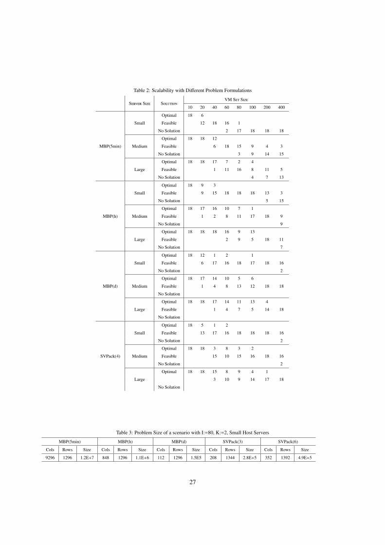
Table 2: Scalability with Different Problem Formulations
Server Size SolutionVM Set Size
10 20 40 60 80 100 200 400
MBP(5min)
Optimal 18 6
Small Feasible 12 18 16 1
No Solution 2 17 18 18 18
Optimal 18 18 12
Medium Feasible 6 18 15 9 4 3
No Solution 3 9 14 15
Optimal 18 18 17 7 2 4
Large Feasible 1 11 16 8 11 5
No Solution 4 7 13
MBP(h)
Optimal 18 9 3
Small Feasible 9 15 18 18 18 13 3
No Solution 5 15
Optimal 18 17 16 10 7 1
Medium Feasible 1 2 8 11 17 18 9
No Solution 9
Optimal 18 18 18 16 9 13
Large Feasible 2 9 5 18 11
No Solution 7
MBP(d)
Optimal 18 12 1 2 1
Small Feasible 6 17 16 18 17 18 16
No Solution 2
Optimal 18 17 14 10 5 6
Medium Feasible 1 4 8 13 12 18 18
No Solution
Optimal 18 18 17 14 11 13 4
Large Feasible 1 4 7 5 14 18
No Solution
SVPack(4)
Optimal 18 5 1 2
Small Feasible 13 17 16 18 18 18 16
No Solution 2
Optimal 18 18 3 8 3 2
Medium Feasible 15 10 15 16 18 16
No Solution 2
Optimal 18 18 15 8 9 4 1
Large 3 10 9 14 17 18
No Solution
Table 3: Problem Size of a scenario with I:=80, K:=2, Small Host Servers
MBP(5min) MBP(h) MBP(d) SVPack(3) SVPack(6)
Cols Rows Size Cols Rows Size Cols Rows Size Cols Rows Size Cols Rows Size
9296 1296 1.2E+7 848 1296 1.1E+6 112 1296 1.5E5 208 1344 2.8E+5 352 1392 4.9E+5
27