Change of Time Methods

in

Quantitative Finance

Anatoliy SwishchukUniversity of Calgary

Department of Mathematics & Statistic2500 University Drive NW

Calgary, AB,Canada T2N 1N4

Preface

”Time changes everything except something within us, which is alwayssurprised, by change”, -Thomas Hardy.

The present book is devoted to the history of change of time methods(CTM), connection of CTM with stochastic volatilities and finance, and manyapplications of CTM. A reader may consider this book as a brief introductionto the theory of CTM and as a handbook that can be used to apply tomany real life problems. As Winston Churchill once said, ’...I only readfor pleasure or for profit,’ similarly, someone may read the present book forpleasure, someone for profit (but see disclaimer below!) and many for both.The author’s intension was to satisfy all the readers who like change of timemethods, stochastic volatilities and finance. There is one book that the mostclose to the present book-’Change of Time and Change of Measure’ by O.Barndorff-Nielsen and A. Shiryaev (Springer, 2010). The difference betweenthe present book and the latter book is that the present book focuses moreon applications and presents some novel models, e.g., the delayed versionof Heston model, that not covered by the monograph of Barndorff-Nielsenand Shiryaev. For some extent, someone may consider the present book as auseful complement to the latter monograph. I hope that the present book willattract a wide audience from graduate students and quants to researchers inmathematical finance, and also to practicioners in finance and energy areas.

Anatoliy SwishchukUniversity of CalgaryCalgary, Alberta, CanadaAugust 2015

Disclaimer

We make no warranties that the approaches contained in this book are free oferror or that they will meet your requirements for any particular application.They should not be relied on for solving a problem, using these approaches,whose incorrect solution could result in loss of money or property. If you douse the approaches, it is at your own risk. The author and publisher disclaimall liability for direct or consequencial damages resulting from your use of theapproaches.

Dedication

To my late parents

Achowledgements

I would like to thank very much to many of my colleagues and graduatestudents, with whom I duscussed or obtained some results presented in thebook, and also to all the participants of the ’Lunch at the Lab’ finance semi-nar at our Department of Mathematics and Statistics, University of Calgary,where all the results were first presented and tested.

Many thanks go to my family, wife Mariya, son Victor and daughter Julia(who found and recommended the picture in the Preface), whose continuoussupport encouraged me on writing and creating.

Chapter 1: Introduction to the Change of Time

Methods: History, Stochastic Volatility, Fi-

nance

”Both Aristotle and Newton believed in absolute time...Time was completelyseparate from and independent of space...However, we have had to change ourideas about space and time...”-Stephen Hawking ’A Brief History of Time’

1 Introduction to the Change of Time Meth-

ods

In this Chapter, we consider a history for the change of time methods (CTM),connection of CTM with finance and stochastic volatilities.

Let (Ω,F ,Ft, P ) be a filtered probability space, t ≥ 0. We shall frequentlyuse in this book the notion of: 1) Brownian motion Bt (or Wiener processWt): a process with independent Gaussian (normal) increments and con-tinuous trajectories (A. Einstein (1905) used it when analysing the chaoticmotion of particles in a liquid); 2) stochastic differential equation dXt =a(Xt, t)dt + σ(Xt, t)dBt (describing diffusion process Xt with drift a anddiffusion σ) with local Lipschitz and linear growth conditions for the coeffi-cients a and σ; 3) martingale Mt (stochastic model for fair game), meaningE|Mt| < +∞ and E(Mt|Fs) = Ms, s ≤ t, where Mt is a stochastic process onthe above mentioned filtered probability space; 4) Levy process Lt (processthat contains deterministic drift, diffusion and jumps) (i.e., stochasticallycontinuous process with stationary and independent increments) (see, e.g.,Jacod & Shiryaev (1987), Applebaum (2003)).

The main idea of change of time method is to find a simple representationfor a stochastic process with a complicated structure, using some simpleprocess and change of time process. For example, if we consider a Brownianmotion Bt (or Levy process Lt) as a simple process and Xt as a complicatedprocess, that satisfies the following stochastic differential equation dXt =a(Xt, t)dt + σ(Xt, t)dBt (or dXt = a(Xt, t)dt + σ(Xt, t)dLt) on the latterfiltered probability space, then the question is: can we represent Xt in thefollowing form

Xt = BTt , (or Xt = LTt)

where Tt is a change of time process? In many cases, the answer is ’yes’.In this book, we shall show you those cases and many applications of them.In general, the procedure of change of time means that we proceed from old(or physical, calendar) time t to a new (operational, business) time t′ witht′ = Tt in a such way to be able to construct our initial complicated processXt (old one) through a simple process Xt (new one) that satisfies the relationXt = XTt . If we define t = T ′

t , then Xt′ = XT ′t, t′ > 0.

1

1.1 A Brief History of Change of Time Method

To the best of the author’s knowledge, Wolfgang Doeblin (see Doeblin W.(1940), Levy (1955), Lindvall (1991) and also Bru and Yor (2002) for details)was the first one who introduced change of time method into the theory ofstochastic processes. He took the martingale point of view in his analysisof the paths of an inhomogeneous real-valued diffusion Xt, t ≥ 0, startingfrom x, with drift coefficient a(x, t) and diffusion coefficient σ(x, t). If wedefine Yt := Xt − x−

∫ t0a(Xs, s)ds and ht :=

∫ t0σ2(Xs, s)ds, then he proved

first that Yt and Y 2t − ht are martingales without mentioning the notion

of martingale (see Doeblin (1940)). Secondly, Doeblin introduced the timechange θ(τ) := inft : mt > τ, τ > 0 and showed that B(τ) := Yθ(τ) isa Brownian motion. In fact, he proved that there exists a Brownian motionB(s), s ≥ 0, such that Yt := B(ht). All in all, Doeblin has obtained therepresentation of Xt as

Xt = x+B(ht) +

∫ t

0

a(Xs, s)ds. (1)

Of course, at that time the general notion of martingale did not exist (seefor more details Bru and Yor (2002)). The notion of positive martingale andits denomination (which Doeblin does not use) are due to Ville, in his 1939thesis (see Ville (1939)) (martingale property was also used by Levy underanother name, ’condition C’, since 1934). A several years later, K. Ito (1942a,1942b (see also Ito (1951a, 1951b)) presented Xt in the form of stochasticdifferential equation

Xt = x+

∫ t

0

a(Xs, s)ds+

∫ t

0

σ(Xs, s)dB(s), (2)

where B(s) is a Brownian motion. If we compare Doeblin’s and Ito’s repre-sentaions (1) and (2), then we can obtain∫ t

0

σ(Xs, s)ds = B(ht). (3)

The latter result (3) would be understood, of course, in a general settingmany years later with the Dambis (1965) and Dubins-Schwartz (1965) rep-resentation of a continuouus martingale Mt as

Mt = B(< M >t), (4)

where B(u) is a Browinian motion and < . > is the quadratic variation. Theidea of associating with a diffusion Xt a compensated process Yt which followsthe trajectories of a standard Brownian motion is presented in the works ofLevy on additive processes (see Levy (1934, 1937, 1948)) and in the seminalpaper of Kolmogorov (1931). However, as Bru and Yor (2002) mentioned,”Doeblin’s method goes much further and the change of time which he adopts

2

seems to be original.It is usually attributed to Volkonskii (1958); see e.g.Dynkin (1965); Williams (1979). In any case, there does not seem to bemuch use for random time-changes in the study of diffusion before the endof the fifties”. Though, we would like to mention that Bochner (1949) alsoused the notion of ’change of time’, namely, time-changed Brownian motion,before the beginning of fifties.

Girsanov (1960) used change of time method to find a nontrivial weaksolution to the following stochastic differential equation dXt = |Xt|αdBt,where X0 = 0, Bt is a Brownian motion and 0 < α < 1/2.

It worth to mention here that the change of time method is closely asso-ciated with the embedding problem: to embed a process X(t) in Brownianmotion is to find a Brownian motion (or Wiener process) B(t) and an in-creasing family of stopping times Tt such that B(Tt) has the same jointdistribution as X(t). Skorokhod (1965) first treated the embedding problem,showing that the sum of any sequence of independent random variables withmean zero and finite variation could be embedded in Brownian motion usingstopping times. See also Monroe (1972).

Dambis (1965), Dubins & Schwartz (1965) independently showed thatevery continuous martingale could be embedded in Brownian motion (inthe sense of (4) above). Feller (1936, 1966) introduced subordinated pro-cess X(Tt) for a Markov process X(t) with Tt a process having indepen-dent increments. Tt was called ’randomized operational time’. Huff (1969)showed that every process of pathwise bounded variation could be embed-ded in Brownian motion. Knight (1971) discovered a multivariate extensionof the Dambis (1965) and Dubins & Schwartz (1965) result. Monroe (1972)proved that every right continuous martingale could be embedded in a Brow-nian motion. Meyer (1971) and Papangelou (1972) independently discoveredKnight’s (1971) result for point processes.

Clark (1973) introduced change of time method into financial economics.Monroe (1978) proved that a process can be embedded in Brownian motionif and only if this process is a local semimartingale. Johnson (1979) intro-duced a time-changed stochastic volatility model in continuous time. Ikeda& Watanabe (1981) introduced and studied the change of time to find thesolutions of stochastic differential equations. Rosinski & Woyczynski (1986)considered time changes for integrals over a stable Levy processes. Levyprocesses can also be used as a time change for other Levy processes (sub-ordinators). Johnson & Shanno (1987) studied pricing of options using atime-changed stochastic volatility model.

Madan & Seneta (1990) introduced variance gamma process (i.e., Brown-ian motion with drift time changed by a gamma process). Kallsen & Shiryaev(2001) showed that the Rosinski-Woyczynski-Kallenberg result can not be ex-tended to any other Levy processes other than the symmetric α-stable pro-cesses.Kallenberg (1992) considered time change representations for stableintegrals. Geman, Madan & Yor (2001) considered time changes (’businesstimes’) for Levy processes .

3

Barndorff-Nielsen, Nicolato & Shephard (2002) studied the relationshipbetween subordination and stochastic volatility models using a change of time(they called it the Tt-’chronometer’). Carr, Geman, Madan, Yor (2003) usedsubordinated processes to construct stochastic volatility for Levy processes,(Tt being ’business time’).

Carr, Geman, Madan & Yor (2003) also used a change of time to introducestochastic volatility into a Levy model to achieve leverage effect and a long-term skew.

Swishchuk (2004) applied change of time method for pricing varinace,volatility, covariance and correlation swaps for Heston model. Change oftime method was applied to option pricing for mean-reverting models inenergy markets in Swishchuk (2008b). Pricing of Levy-based interest ratederivatives based on change of time method was considered in Swishchuk(2008a). An overview of change of time method in mathematical finance andits applications was presented in Swishchuk (2007). Applications of changeof time method to multi-factor Levy-based model for pricing of financial anaenergy derivatives was considered in Swishchuk (2009).

The book ’Option Prices as Probabilities’ by C. Profeta, B. Roynette andM. Yor (Springer, 2010) is also relies on time change methods.

The recent book ’Change of Time and Change of Measure’ by Barndorff-Nielsen and Shiryaev (2010) states the main ideas and results of the stochastictheory of ’change of time and change of measure’.

1.2 Change of Time Method and Stochastic Volatility

The volatility is a measure for variation of price St of a financial instrumentover time t ≥ 0. We use the symbol σ for volatility and it corresponds tostandard deviation which quantifies the amount of variation or dispersionof a set of data values St. Of course, σ can be positive constant, positivedeterministic function of time σ(t) or a stochastic process σ(t, ω), ω ∈ Ω, e.g.,that satisfies some stochastic differential equation. The model for volatilitythat initiated the stochastic volatility model was implied volatility model:this volatility σ ≡ σ(K,T ) can be derived from the Black-Scholes formulafor the European call option price and demonstrates the smile effect, e.g.,dependency of volatility from strike price K and maturity T (see Fouque,Papanicolaou and Sircar (2000)). This smile effect tells us that the Balck-Scholes model with a constant volatility is not adequate to statistical andprobabilitical structures of observable prices St. Merton (1973) was the firstone who replaced the constant volatility σ by a deterministic function σ =σ(t), t ≥ 0. In such models there is no smile effect across strike, howeversmile effect appears for different maturiries. Another way to obtain smileeffect with nonstochastic volatility is to add to the deterministic volatilityσ(t) one more variable, namely, phase one, S : σ ≡ σ(t, S) (see Dupire(1994)). We can go further and assume that volatility depends not onlyfrom t and S, but also on all proceding values Su, u ≤ t, i.e., the volatility

4

σ(t, Su;u ≤ t)) depends on all past observed prices, or volatility dependson its own past values. The latter case will be considered in Chapter 8.Besides smile effect, mean reversion (i.e., returning of the volatility to themean) is another important property of stochastic volatility. That’s why mostof modern models of stochastic volatility are assumed that the volatility isgenerated by another source of randomness than initial Brownian motion Bt,say by process Yt, which correlates with Bt, and this process follows somemean-reversion process, say, Ornstein-Uhlenbeck or CIR process (see Contand Tankov (2004)).

The connection of change of time with stochastic volatility can be de-scribed by the following representation: Xt = XT (t) =

∫ t0σ(s, ω)dXs, where

Xt is a given process, σ(t, ω) is a stochastic volatility, Xt is a simple initialprocess and T (t) is a change of time process. In many cases in finance, theprocess Xt is a Brownian motion or Levy process. In general case, the processXt is a semimartingale, meaning Xt = X0 +At+Mt, where At is a process ofbounded variation and Mt is a local martingale (see, e.g., Barndorff-Nielsenand Shiryaev (2010)).

The most typical example of this connection between change of timeand stochastic volatility is the following one. Let Mt =

∫ t0σ(s, ω)dBs, t ≥

0, where Bs is a Brownian motion, σ(s, ω) is a positive process such that∫ t0σ2sds < +∞. Then Mt can be presented in the following way:

Mt = BTt ,

where Tt :=∫σ2sds, Bt := MTt

, and Tt = infs :∫ s0σ2udu ≥ t. We note that

Bt := MTtis a Brownian motion with respect to the filtration Ft := FTt .

Another interesting example associated with the α-stable processes Lαs , 0 <α ≤ 2 (see Applebaum (2003)). LetXt =

∫ t0σ(s, ω)dLαs , T (t) :=

∫ t0|σ(s, ω)|αds <

+∞, and Tt = infs ≥ 0 : Ts > t. Then

Lαt := XTt, t ≥ 0,

is an α-stable process. The proof follows from the Doob optional samplingtheorem and the characteristic property of semimartingales (see Jacod &Shiryaev (1987)). We note that processXt can be represented through changeof time in the following way:

Xt = LαTt .

We shall use this approach in Chapters 6 and 7 for Levy-based and multi-factor financial models.

It is worth to mention that the only change of time process Tt that re-tains the Gaussian property of the time changed Brownian motion BTt isdetrministic one.

The probability literature has demonstrated that stochastic volatilitymodels and their time-changed Brownian motion relatives are fundamental(see Shephard (2005a, 2005b)).

5

1.3 Change of Time Method and Finance

The change of time method in finance is related directly to the notion ofvolatility, the measure for variation of price of a financial instrument (stock,etc.) over time t ≥ 0. Often the change of time is called an ’operational time’(the term first coined by Felller (1966)) or ’business time’ (Carr, Madan &Yor (2001)). This time measures the intensity of the variations/fluctuationsof the prices in the financial markets. The notion of change of time is veryimportant in finance because many prices in the financial markets can beexpressed in the form of Brownian motion with the changed time, called theoperational or business time.

The role of Brownian motion in finance is also hard to underestimate:besides its important role in probability and stochastic processes (centrallimit theorem, functional limit theorem and so-called time-changed Brownianmotion processes), it was the main component in modeling of the dynamicsof financial asset prices St, t ≥ 0. We would like to mention Bachelier model(1900) St = S0 +µt+σBt and Samuelson model (1965) log St

S0= µt+σBt for

asset prices St, where Bt is a Brownian motion. Another important processin finance is Poisson process, antipode to Brownian motion, which was firstused by Lundberg (1903) to model the dynamics of the capital of insurancecompanies.

Both Brownian motion and Poisson process are main components in con-structing more general class of processes in finance and insurance, Levy pro-cesses (see Levy (1934, 1935, 1937, 1954), Applebaum (2003)). To go fur-ther, we mention that even more general processes recently have been usedto construct many financial and insurance model, namely, processes with in-dependent increments and semimartingales (see Shiryaev (2008)). The latterprocesses are not necessarily homogeneus as in the case of Levy processes.As we can see later, we can obtain these kind of processes in finance if weconsider Bachelier (1903) and Samuelson (1965) models, mentioned above, inchange of time mode, namely, St = S0+µT (t)+σBTt and log St

S0= µTt+σBTt ,

respectively, where Tt is a change time process. Another important examplein finance can be constructed if we take gamma process Tt and a Brown-ian motion B(t), independent of each other, and then form a new processG(t) such that G(t) = µt + βTt + BTt . This process is called the variancegamma process (or VG process) (see Madan & Seneta (1990)). To catchthe leverage and clustering effects, other models of stock prices in financecan be obtained using, for example, exponential Levy models that includeboth stochastic volatility and change of time, and also the models based onfractional Brownian motion (see Barndorff-Nielsen and Shiryaev (2010)).

Many stochastic differential equations, that practicioners use in finance,can be solved using chnage of time method as well. One of such equations isOrnstein-Uhlenbeck equation (see Ornstein & Uhlenbeck (1930)) (we presentthis equation in general form):

dXt = (a(t)− b(t)Xt)dt+ c(t)dW (t),

6

where W (t) is a Wiener process (or Brownian motion) and a, b, c are deter-ministic functions of time t ≥ 0. The solution of this equation is:

Xt = exp(−∫ t

0

b(s)ds)[X0+

∫ t

0

a(s) exp(

∫ s

0

b(u)du)ds+

∫ t

0

c(s) exp(

∫ s

0

b(u)du)dWs].

The solution of this equation can also be presented in the following form,using chnage of time method (see Swishchuk (2007) and Ikeda & Watanabe(1981)):

Xt = exp(−∫ t

0

b(s)ds)[X0 +

∫ t

0

a(s) exp(

∫ s

0

b(u)du)ds+BTt ],

where Tt =∫ t0(c(s)) exp(

∫ s0b(u)du))2ds-change of time process, and Bt is a

new Brownian motion. The latter Brownian motion can be obtained fromthe previous one, W (t), by the following formulae:

Bt :=

∫ Tt

0

c(s) exp(

∫ s

0

b(u)du)dW (s),

where Tt = infs : Ts > t, where Tt is defined above.We shall use this approach in the next Chapter 2 to find the solutions of

many stochastic differential equations.

2 Structure of the Book

Chapter 2 is devoted to the general theory of change of time method andmany approaches in this field.

Chapter 3 gives yet one more derivation (among many others) of Black-Scholes option pricing formula using change of time method. In this chapterwe also present a brief introduction to the option pricing theory.

Chapter 4 models and prices variance, volatility, covariance and corre-lation swaps for classical Heston model of a stock price. We also give anumerical example based on S&P60 Canada Index.

Chapter 5 introduces a new delayed Heston model for pricing of varianceand volatility swaps, and also for hedging volatility swaps using varianceswaps. We use here change of time method as well, and also calibrate all theparameters based on real data. This model improves the market volatilitysurface fitting by 44% compare with classical Heston model.

Chapters 6 introduces multi-factor Levy-based financial and energy mod-els. Change of time method is used to price many financial and energyderivatives.

Chapter 7 deals with explicit option pricing formula for a mean-revertingasset in energy markets using change of time method. We also present herea numerical example for AECO natural gas index.

7

Finally, Chapter 8 deals with variance and volatility swpas in energymarkets using CTM as well.

All chapters contain their own list of References.Warning!: We note that we use throughout the book two notations for

the change of time process, namely, Tt and φt, with respect to Barndorff-Nielsen and Shiryaev’s and Ikeda and Wananabe’s books. For example, inChapters 1,2 and 7 we use Tt and in Chapters 3-5 and 8 we use φt.

3 References

Applebaum, D. Levy Processes and Stochastic Calculus, Cambridge Uni-versity Press, 2003.

Bachelier, L. Theorie de la speculation. Ann. Ecole Norm. Sup. 17,(1900), 21-86.

Barndorff-Nielsen, O.E., Nicolato, E. and Shephard, N. Some recent de-velopment in stochastic volatility modeling, Quantitative Finance, 2, 11-23,2002.

Barndorff-Nielsen, O. E. and Shiryaev, A. N. Change of Time and Changeof Measure. World Scientific. Singapore, 2010, 305 p..

Bochner, S. Diffusion equation and stochastic processes. Proc. Nat.Acad. Sci. USA, 85, 369-370, 1949.

Bru, B. and Yor, M. Comments on the life and mathematical legacy ofWolfgang Doeblin. Finance and Stochastics, 6, 3-47 (2002).

Carr, P., Geman, H., Madan, D. and Yor, M. Stochastic volatility for Levyprocesses.// Mathematical Finance, vol. 13, No. 3 (July 2003), 345-382.

Clark, P. A subordinated stochastic process model with fixed variance forspeculative prices, Econometrica, 41, 135-156, 1973.

Cont, R. and Tankov, P. Financial Modeling with Jump Processes, Chap-man & Hall/CRC Fin. Math. Series, 2004.

Dambis, K.E. On the decomposition of continuous submartingales, The-ory Probabability and its Appl., 10, 4091-410, 1965.

Doeblin, W. Sur l’equation de Kolmogoroff. Pli cachete depose le 26fevrier 1940, ouvert le 18 mai 2000. C.R. Acad. Sci. Paris, Series I, 331,1031-1187 (2000).

Dubins, L. and Schwartz, G. On continuous martingales, Proc. Nat.Acad. Sciences, USA, 53, 913-916, 1965.

Dupire, B. Pricing with a smile. Risk, 7,1, 18-20 (1994).Dynkin, E. B. Markov Processes. vol. 2. Berlin-Heidelberg-New York:

Springer, 1965.Einstein, A. Uber die von der molekularkinetischen Theorie der Warme

geforderte Bewegung von in rehunden Flussigkeiten suspendierten Teilchen,Ann. Phys. (4) 17, 549-560 (1905).

8

Feller, W. Zur der stochastischen prozesse (Existenz-und Eindeutigkeitssatze).Math. Ann., 113, 113-160 (1936).

Feller, W. Introduction to Probability Theory and its Applications, v. II,Wiley & Sons, 1966.

Fouque, J.-P., Papanicolaou, G. and Sircar, K. R. Derivatives in FinancialMarkets with Stochastic Volatilities. Springer-Verlag, 2000.

Geman, H., Madan, D. and Yor, M. Time changes for Levy processes,Math. Finance, 11, 79-96 (2001).

Girsanov, I. On transforming a certain class of stochastic processes by ab-solutely continuous subtitution of measures. Theory Probab. Appl., 5(1960),3, 285-301.

Heston, S. A closed-form solution for options with stochastic volatilitywith applications to bond and currency options, Review of Financial Studies,6, 327-343, 1993.

Huff, B. The loose subordination of differential processes to Brownianmotion, Ann. Math. Statist., 40, 1603-1609.

Ikeda, N. Watanabe, S. Stochastic Differential Equations and DiffusionProcesses. North-Holland/Kodansha Ltd., Tokyo, 1981.

Ito, K. Differential equations determining a Markoff proces.. J. Pan-JapanMath. Colloq. 1077, 1352-1400 (in Japanese) (1942a).

Ito, K. On stochastic processes (I) (Infinitely divisible laws of probability).Japan J. Math. 18, 261-301 (1942b)

Ito, K. On stochastic differential equations. Mem. Amer. Math. Soc., 4(1951a).

Ito, K. On a formula concerning stochastic differentials. Nagoya Math.J., 3, 55-65 (1951b).

Jacod, J. and Shiryaev, A. Limit Theorems for Stochastic Processes.Springer-Verlag, 1987.

Johnson, H. Option pricing when the variance rate is changing. Workingpaper, University of california, Los Angeles, 1979.

Johnson, H. and Shanno, D. Option pricing when the variance is changing,J. Financial Quant. Anal., 22, 143-152 (1987).

Kallenberg, O. Some time change representations of stable integrals, viapredictable transformations of local martingales. Stochastic Processes andTheir Applications, 40 (1992), 199-223.

Kallsen, J. and Shiryaev, A. Time change representation of stochasticintegrals, Theory Probab. Appl., vol. 46, N. 3, 522-528, 2002.

Khinchin A. Y. Asymptotische gesetze der Warsheinlichkeitsrechnung.Berlin-Heidelberg-New York: Springer, 1933 (Ergebnisse der Mathematikund ihrer Grenzgebiete, vol. 2, no. 4) (Reprint, New York: Chelsea, 1948).

Knight, F. A reduction of continuous, square-integrable martingales toBrownian motion, in: H. Dinges, ed., Martingales, Lecture Notes in Math.No. 190 (Springer, Berlin, 1971) pp. 19-31.

Kolmogorov A. N. Uber die analytischen methoden in der Wahrschein-lichkeitsrechnung. Math. Ann., 104, 149-160 (1931).

9

Levy, P. Sur les integrals dont les elements sont des variables aleatoiresindependentes. Ann. J. Sc. Norm. Sup. Pisa S. 2 (3), 337-366 (1934), 4,217-218 (1935).

Levy, P. Theorie de l’addition des variables aleatoires, Paris: Gauthier-Villars, 1937 (2nd edn. ibid, 1954).

Levy, P. Processus Stochastiques et Mouvement Brownian, 2nd ed., Gauthier-Villars, Paris, 1948 (2nd edn. ibid, 1954).

Levy, P. Wolfgang Doeblin (V. Doblin)(1915-1940). Rev. Histoire Sci.107-115 (1955).

Lindvall, T. W. Doeblin 1915-1940. Ann. Prob., 19, 929-934 (1991).Lundberg, F. Approximerad Framstallning Sannolikhetsfunktionen. II.

Aterforrsakering av Kolletivrisker. Akad. Afhandling. (Almqvist&Wiksell,Uppsala), (1903)

Madan, D. and Seneta, E. The variance gamma (VG) model for sharemarket returns, J. Business 63, 511-524, (1990).

Merton, R. Theory of rational option pricing. Bell J. Econ. and Man-agement Sci., 4, 141-183 (1973).

Meyer, P. A. Demonstration simplifiee d’un theoreme de Knight, in: Sem-inaire de Probabilites V, Lecture Notes in Math. No. 191 (Springer, Berlin,1971) pp. 191-195.

Monroe, I. On embedding right continuous martingales in Brownian mo-tion, Ann. Math. Statist., 43, 1293-1311, 1972.

Monroe, I. Processes that can be embedded in Brownian motion, TheAnnals of Probab., 6, No. 1, 42-56, 1978.

Ornstein, L. and G.Uhlenbeck. On the theory of Brownian motion. Phys-ical Review, 36 (1930), 823-841.

Papangelou, F. Integrability of expected increments of point processesand a related random change of scale, Trans. Amer. Math. Soc., 165 (1972)486-506.

Profeta, B., Roynette, B. and Yor, M. Option Prices as Probabilities.Springer-Verlag, Berlin-Hedelberg, 2010.

Rosinski, J. and Woyczinski, W. On Ito stochastic integration with re-spect to p-stable motion: Inner clock, intagrability of sample paths, doubleand multiple integrals, Ann. Probab., 14 (1986), 271-286

Samuelson, P. Rational theory of warrant pricing. Industrial ManagementRev., 6, (1965), 13-31.

Shephard, N. Stochastic Volatility: Selected Readings. Oxford: OxfordUniversity Press, 2005a.

Shephard, N. Stochastic Volatility. Working paper, Oxford: Oxford Uni-versity Press, 2005b.

Shiryaev, A. Essentials of Stochastic Finance, World Scientific, 2008.Skorokhod, A. Random Processes with Independent Increments, Nauka,

Moscow, 1964. (English translation: Kluwer AP, 1991).Skorokhod, A. Studies in the Theory of Random Processes, Addison-

Wesley, Reading, 1965.

10

Swishchuk, A. Modelling and valuing of variance and volatility swaps forfinancial markets with stochastic volatilites, Wilmott Magazine, TechnicalArticle, N0. 2, September, 2004, 64-72.

Swishchuk, A. Change of time method in mathematical finance, Canad.Appl. Math. Quart., vol. 15, No. 3, 2007, 299-336.

Swishchuk, A. Levy-based interest rate derivatives: change of time andPIDEs, Canad. Appl. Math. Quart., v. 16. No. 2, 2008a.

Swishchuk, A. Explicit option pricing formula for a mean-reverting assetin energy market, J. of Numer. Appl. Math., Vol. 1(96), 2008b, 216-233.

Swishchuk, A. Multi-factor Levy models for pricing of financial and energyderivatives, Canad. Appl. Math. Quart., v. 17, N0. 4, 2009.

Ville, J. Etude critique de la notion de collectif, These sci. math. Paris,(fascicule III de la Collection de monographies des probabilites, publiee sousla direction de M. Emile Borel). Paris: Gautier-Villars, 1939.

Volkonskii, V. A. Random substitution of time in strong Markov pro-cesses. Teor. Veroyatnost. i Primenen., 3, 332-350 (1958).

Williams, D. Diffusion, Markov Processes and Martingales I. Fiundations.New York, Wiley, 1979.

11

Chapter 2: Change of Time Methods: Defini-

tions, Theory and Applications

’It is always more easy to discover and proclaim general principles than toapply them’,-Winston Churchill.

1 Change of Time Methods: Definitions, Prop-

erties and Theory

In this Chapter, we consider a general theory of change of time method.One of probabilistic methods which is useful in solving stochastic differentialequations (SDEs) arising in finance is the change of time method. In thisIntroduction we give definition of CT, describe CTM in martingale, semi-martingale and the SDEs settings. We also point out the association ofCTM with subordinators and stochastic volatilities. Applications of CTMsuch as Black-Scholes formula, option pricing formula for a mean-revertingasset, variance and volatility swap prices for Heston and delayed Heston mod-els, and variance and volatility swap prices in energy markets are describedas well.

1.1 Change of Time Process: Definition and Proper-ties

Let (Ω,F ,Ft, P ) be a filtered probability space with a sample space Ω, σ-algebra F of subsets of Ω and probability measure P. The filtration Ft, t ≥0, is a nondecreasing right-continuous family of sub-σ-algebras of F .

Definition of Change of Time Process. A time change process is aright-continuous increasing [0,+∞]-valued and Ft-adapted process (Tt)t∈R+

such that limt→+∞ = +∞. Tt is also a stopping time for any t ∈ R+.By Ft := FTt we define the time-changed filtration (Ft)t∈R+ . The inverse

time change (Tt)t∈R+ is defined as Tt := infs ∈ R+ : Ts > t. We note

that Tt is increasing process and limt→+∞ Tt = +∞. Furthermore, Tt is anFt-stopping time. Let Xt be an Ft-adapted process and define XTt

. Then

XTtis Ft-adapted process and this process is called the time change of Xt

by Tt.One of the examples of change of time is the following. Let At be an Ft-

adapted, increasing, right-continuous random process with A0 = 0. Define

Tt = infs : As > t, t ≥ 0.

Then the process Tt is a change of time process. We call At as the processgenerating the change of time Tt. We note that the process Tt (see abovedefinition) coincides with At in this case. It means that changes of time

12

processes Tt and Tt are mutually inverse processes: someone may constructTt using Tt,

Tt = infs : Ts > t,or, may construct Tt using Tt :

Tt = infs : Ts > t.We also note that

TTt = t and TTt = t.

We would like to also mention the change of time in Lebesque-Stiltjes inte-grals, which is well-known from calculus. If we take At, A0 = 0, as a deter-ministic increasing continuous function, f(t) as a nonnegative Borel functionon [0,+∞), and put

At = infs : As > t,then we have ∫ Aa

0

f(t)dAt =

∫ a

0

f(At)dt, a > 0.

We note that At =∫s : As > t and AAt

= t. The latter expression can bewritten in the symmetric form as well:∫ Aa

0

f(t)dAt =

∫ a

0

f(At)dt, a > 0.

There are many stochastic generalizations of the last two relationships for thecase of A and f being some stochastic processes. One of them is the folllowingone: let f(t, ω) be a progressively measurable nonegative stochastic process,and let Bt(ω) be an Ft-measurable right-continuous process with boundedvariation. Then ∫ Ta

0

f(t, ω)dBt(ω) =

∫ a

0

f(Tt, ω)dBTt(ω),

where Tt is the inverse change of time process. For example, if f(t, ω) =F (T (t)), where Tt = At, and At is a continuous and strictly increasing processgenerating the change of time Tt (see above), then∫ Ta

0

F (Tt)dBt(ω) =

∫ a

0

F (t)dBTt(ω).

Of course, if Bt = t, then∫ Ta

0

F (Tt)dt =

∫ a

0

F (t)dTt,

and, if Bt = Tt, then ∫ Ta

0

F (Tt)dTt =

∫ a

0

F (t)dt.

See Ikeda and Watanabe (1981) and Barndorff-Nielsen and Shiryaev (2010)for more details.

13

1.2 CTM: Martingale and Semimartingale Settings

The general theory of time changes for martingale and semimartingale the-ories is well known (see Ikeda and Watanabe (1981)). We will give a briefoverview of those results.

The following result on martingales and change of time process belongsto Dambis (1965) and Dubins and Schwartz (1965): Suppose Mt is squareintegrable local continuous martingale such that limt→+∞ < M > (t) = +∞a.s., and define Tt := infu :< M >u> t and Ft = FTt . Then the time

changed process B(t) := MTtis an Ft-Brownian motion. Also, Mt = B(<

M >t). Thus, Mt can be presented by an Ft-Brownian motion B(t) andan Ft-stopping time < M >t . Here, < · > defines predictable quadraticvariation. One of the examples of this result was considered in section 1.2. fora continuous local martingale Mt =

∫ t0σs(ω)dB(s), where Bt is a Brownian

motion and σt(ω) is a positive process such that∫ t0σ2s(ω)ds < +∞. In tis

case, Tt = infs :∫ s0σ2u(ω)du ≥ t and Tt =

∫ t0σ2s(ω)ds.

This result was generalized by Knight (1971) for d-dimensional case: LetM i

t be square integrable local continuous martingales, i = 1, 2, ..., d, suchthat < M i,M j >t= 0 if i 6= j and limt→+∞ < M i >t= +∞ a.s. If T it =

infu :< M i >u> t, then ~B(t) = (B1(t), B2(t), ..., Bd(t)) is a d-dimensionalBrownian motion, where Bi(t) = M i

T it

, i = 1, 2, ..., d.

One of the main properties of semimartingale Xt with respect to the CTMis the following (see Liptser and Shiryaev (1989)): If Xt is a semimartingalewith respect to a filtration Ft, then the changed time process XTt

is also a

semimartingale with respect to the filtration Ft (see sec. 1.1).If we have the triplet of predictable characteristics (Bt, Ct, ν) for a semi-

martingale Xt, then the triplet of the time changed semimartingale XTtis

determined as (BTt, CTt , IGνTt) (see Kallsen and Shiryaev (2001)).

The connection of semimartingales, Brownian motions and CTM is de-scribed by the Monroe result (see Monroe (1978)): if Xt is a semimartingale,then there exists a filtered probability space with Brownian motion Bt anda change of time Tt on it such that distribution of Xt coincides with thedistribution of BTt , namely,

Xt =law BTt . (1)

Let us consider now a counting process Nt with respect to the filtrationFt and with the continuous compensator At such that Nt = At +Mt, whereMt is a local martingale. Here, < M >= A. Let us then define time changeas Tt = infs :< M >s> t. If we suppose that < M >+∞= +∞, then thefollowing process

Nt := NTt

is a standard Poisson process with the intensity parameter λ = 1. We notethat the initial counting process Nt can be expressed in the following way:

Nt = NTt ,

14

where Tt =< M >t . We note that here Mt = MTt , where Mt = Nt − t is aPoisson martingale (see Liptser and Shiryaev (2001) for more detauls).

Suppose that we have a nondecreasing Levy process Xt and a Brownianmotion Bt independent of Xt. Then we can find a change of timne Tt suchthat

Xt = BTt (2)

holds with probability one. This change of time Tt can be found as

Tt = infs : Bs = Xt.

We mention that a semimartingale Xt can be presented in the form (1) withcontinuous change of time Tt if and only if the process Xt is a continuouslocal martingale (see Huff (1969) and Cherny and Shiryaev (2002) for moredetails).

1.3 CTM: Subordinators and Stochastic Volatility

We note, that if the process Tt (see sec. 1.1) is a Levy process, then Tt iscalled subordinator. Feller (1966) introduced a subordinated process Xτt fora Markov process Xt and τt a process with independent increments. τt wascalled a ‘randomized operational time‘. Increasing Levy processes can alsobe used as a time change for other Levy processes (see Applebaum (2004),Barndorf-Nielsen et al. (2001), Barndorf-Nielsen et al. (2003), Bertoin(1996), Cont et al. (2004) and Schoutens (2003)). Levy processes of this kindare called subordinators. They are very important ingredients for buildingLevy based models in finance (see Cont et al. (2004) and Schoutens (2003)).If St is a subordinator, then its trajectories are almost surely increasing, andSt can be interpreted as a ‘time deformation‘ and used to ‘time change‘ otherLevy processes. Roughly, if (Xt)t≥0 is a Levy process and (St)t≥0 is a sub-ordinator independent of Xt, then the process (Yt)t≥0 defined by Yt := XSt

is a Levy process (see Cont et al. (2004)). This time scale has the finan-cial interpretation of business time (see Geman et. al. (2001)), that is, theintegrated rate of information arrival. Using subordinator St and a Brow-nian motion Bt that is independent of Stwe can construct many stochasticprocesses Xt = BSt . For example: for Cauchy process St = infs : Bs > t,where Bs is a standard Brownian motion independent of Bt; for generalizedhyperbolic Levy processes St is generated by the nonnegative infinitely divis-ible random variable having generalized inverse Gaussian distribution (thenormal inverse Gaussian and hyperbolic Levy processes are particular casesof the generalized hyperbolic Levy processes).

The time change method was used to introduce stochastic volatility into aLevy model to achieve the leverage effect and a long-term skew (see Carr et.al. (2003)). In the Bates (1996) model the leverage effect and long-term skewwere achieved using correlated sources of randomness in the price process and

15

the instantaneous volatility. The sources of randomness are thus required tobe Brownian motions. In the Barndorff-Nielsen et al. (2001, 2002) model theleverage effect and long-term skew are generated using the same jumps in theprice and volatility without a requirement for the sources of randomness to beBrownian motions. Another way to achieve the leverage effect and long-termskew is to make the volatility govern the time scale of the Levy process drivingjumps in the price. Carr et al. (2003) suggested the introduction of stochasticvolatility into an exponential-Levy model via a time change. The genericmodel here is St = exp(Xt) = exp(Yvt), where vt :=

∫ t0σ2sds. The volatility

process should be positive and mean-reverting (i.e., an Ornstein-Uhlenbeckor Cox-Ingersoll-Ross processes). Barndorff-Nielsen et al.(2003) reviewed andplaced in the context some of their recent work on stochastic volatility modelsincluding the relationship between subordination and stochastic volatility.

In general setting, the connection between stochastic volatility and changeof time can be described in the following way. Let Xt =

∫ t0HsdBs, where

Hs is the adapted process such that∫ t0H2sds < +∞,

∫ +∞0

H2sds = +∞, and

Bt is a Brownian motion. Then the process Bt := XTt, where Tt = infs :<

X >s> t, is a Brownian motion. Moreover, the process Xt has the followingrepresentation Xt = BTt , where Tt =< X >t=

∫ t0H2sds.

In the case of α-stable processes Y αt instead of Brownian motion Bt in the

integral Xt =∫ t0HsdY

αs , we have similar result for Tt =

∫ t0|Hs|αds < +∞

and∫ +∞0|Hs|αds = +∞. If we set Tt = infs : Ts >> t, then Y α

t = XTtis

an α-stable process and Xt = Y αTt.

The main difference between the change of time method and the sub-ordinator method is that in the former case the change of time process Ttdepends on the process Xt, but in the latter case, the subordinator St andLevy process Xt are independent.

1.4 CTM: Stochastic Differential Equations (SDEs) Set-ting

1.4.1 General Result

We consider the following generalization of the previous results to the SDEof the following form (without a drift)

(2.1) dX(t) = α(t,X(t))dW (t),

where W (t) is a Brownian motion and α(t,X) is a continuous and measurableby t and X function on [0,+∞)×R.

The reason to consider this equation is the following one: if we solve theequation, then we can solve and more general equation with a drift β(t,X)by drift transformation method or Girsanov transformation (see Ikeda andWatanabe (1981), Chapter 4, Section 4]).

16

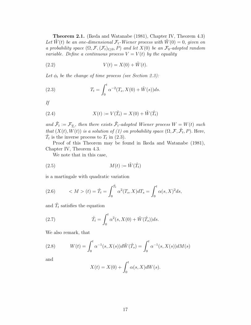
Theorem 2.1. (Ikeda and Watanabe (1981), Chapter IV, Theorem 4.3)Let W (t) be an one-dimensional Ft-Wiener process with W (0) = 0, given ona probability space (Ω,F , (Ft)t≥0, P ) and let X(0) be an F0-adopted randomvariable. Define a continuous process V = V (t) by the equality

(2.2) V (t) = X(0) + W (t).

Let φt be the change of time process (see Section 2.3):

(2.3) Tt =

∫ t

0

α−2(Ts, X(0) + W (s))ds.

If

(2.4) X(t) := V (Tt) = X(0) + W (Tt)

and Ft := FTt , then there exists Ft-adopted Wiener process W = W (t) such

that (X(t),W (t)) is a solution of (1) on probability space (Ω,F , Ft, P ). Here,Tt is the inverse process to Tt in (2.3).

Proof of this Theorem may be found in Ikeda and Watanabe (1981),Chapter IV, Theorem 4.3.

We note that in this case,

(2.5) M(t) := W (Tt)

is a martingale with quadratic variation

(2.6) < M > (t) = Tt =

∫ Tt

0

α2(Ts, X)dTs =

∫ t

0

α(s,X)2ds,

and Tt satisfies the equation

(2.7) Tt =

∫ t

0

α2(s,X(0) + W (Ts))ds.

We also remark, that

(2.8) W (t) =

∫ t

0

α−1(s,X(s))dW (Ts) =

∫ t

0

α−1(s,X(s))dM(s)

and

X(t) = X(0) +

∫ t

0

α(s,X)dW (s).

17

1.4.2 Corollary.

The solution of the following SDE

(2.9) dX(t) = a(X(t))dW (t)

may be presented in the following form

X(t) = X(0) + W (Tt),

where a(X) is a continuous measurable function, W (t) is an one-dimensionalFt-Wiener process with W (0) = 0, given on a probability space (Ω,F , (Ft)t≥0, P )and let X(0) is an F0-adopted random variable. In this case,

(2.10) Tt =

∫ t

0

a−2(X(0) + W (s))ds,

and

(2.11) Tt =

∫ t

0

a2(X(0) + W (Ts))ds.

(See Ikeda and Watanabe (1981), Chapter IV, Example 4.2).We note that

M(t) := W (Tt)

is a martingale with quadratic variation

< M > (t) = Tt =

∫ Tt

0

a2(X)dTs =

∫ t

0

a(X)2ds.

We also remark, that

W (t) =

∫ t

0

a−1(X(s))dW (Ts) =

∫ t

0

a−1(X(0) + W (Ts)))dW (Ts)

and

X(t) = X(0) +

∫ t

0

a(X(s))dW (s).

1.4.3 One-factor Diffusion Models and their Solutions Using CTM

In this section, we introduce well-known one-factor diffusion models (usedin finance) described by SDEs and driven by a Brownian motion (so-calledGaussian models).

For one-factor Gaussian models we define the following well-known pro-cesses:

1. The Geometric Brownian Motion: dS(t) = µS(t)dt+ σS(t)dW (t);

18

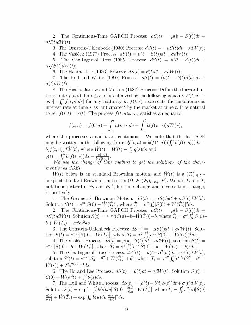
2. The Continuous-Time GARCH Process: dS(t) = µ(b − S(t))dt +σS(t)dW (t);

3. The Ornstein-Uhlenbeck (1930) Process: dS(t) = −µS(t)dt+σdW (t);4. The Vasicek (1977) Process: dS(t) = µ(b− S(t))dt+ σdW (t);5. The Cox-Ingersoll-Ross (1985) Process: dS(t) = k(θ − S(t))dt +

γ√S(t)dW (t);6. The Ho and Lee (1986) Process: dS(t) = θ(t)dt+ σdW (t);7. The Hull and White (1990) Process: dS(t) = (a(t) − b(t)S(t))dt +

σ(t)dW (t);8. The Heath, Jarrow and Morton (1987) Process: Define the forward in-

terest rate f(t, s), for t ≤ s, characterized by the following equality P (t, u) =exp[−

∫ utf(t, s)ds] for any maturity u. f(t, s) represents the instantaneous

interest rate at time s as ‘anticipated‘ by the market at time t. It is naturalto set f(t, t) = r(t). The process f(t, u)0≤t≤u satisfies an equation

f(t, u) = f(0, u) +

∫ t

0

a(v, u)dv +

∫ t

0

b(f(v, u))dW (v),

where the processes a and b are continuous. We note that the last SDEmay be written in the following form: df(t, u) = b(f(t, u))(

∫ utb(f(t, s)))ds+

b(f(t, u))dW (t), where W (t) = W (t)−∫ t0q(s)ds and

q(t) =∫ utb(f(t, s))ds− a(t,u)

b(f(t,u)).

We use the change of time method to get the solutions of the above-mentioned SDEs.

W (t) below is an standard Brownian motion, and W (t) is a (Tt)t∈R+-

adapted standard Brownian motion on (Ω,F , (Ft)t∈R+ , P ). We use Tt and Ttnotations instead of φt and φ−1t , for time change and inverse time change,respectively.

1. The Geometric Brownian Motion: dS(t) = µS(t)dt + σS(t)dW (t).Solution S(t) = eµt[S(0) + W (Tt)], where Tt = σ2

∫ t0[S(0) + W (Ts)]

2ds.2. The Continuous-Time GARCH Process: dS(t) = µ(b − S(t))dt +

σS(t)dW (t). Solution S(t) = e−µt(S(0)−b+W (Tt))+b, where Tt = σ2∫ t0[S(0)−

b+ W (Ts) + eµsb)2ds.3. The Ornstein-Uhlenbeck Process: dS(t) = −µS(t)dt + σdW (t), Solu-

tion S(t) = e−µt[S(0) + W (Tt)], where Tt = σ2∫ t0(eµs[S(0) + W (Ts)])

2ds.4. The Vasicek Process: dS(t) = µ(b−S(t))dt+σdW (t), solution S(t) =

e−µt[S(0)− b+ W (Tt)], where Tt = σ2∫ t0(eµs[S(0)− b+ W (Ts)] + b)2ds.

5. The Cox-Ingersoll-Ross Process: dS2(t) = k(θ−S2(t))dt+γS(t)dW (t),solution S2(t) = e−kt[S2

0 − θ2 + W (Tt)] + θ2, where Tt = γ−2∫ t0[ekTs(S2

0 − θ2 +

W (s)) + θ2e2kTs ]−1ds.6. The Ho and Lee Process: dS(t) = θ(t)dt + σdW (t). Solution S(t) =

S(0) + W (σ2t) +∫ t0θ(s)ds.

7. The Hull and White Process: dS(t) = (a(t)− b(t)S(t))dt+σ(t)dW (t).

Solution S(t) = exp[−∫ t0b(s)ds][S(0)−a(s)

b(s)+W (Tt)], where Tt =

∫ t0σ2(s)[S(0)−

a(s)b(s)

+ W (Ts) + exp[∫ s0b(u)du]a(s)

b(s)]2ds.

19

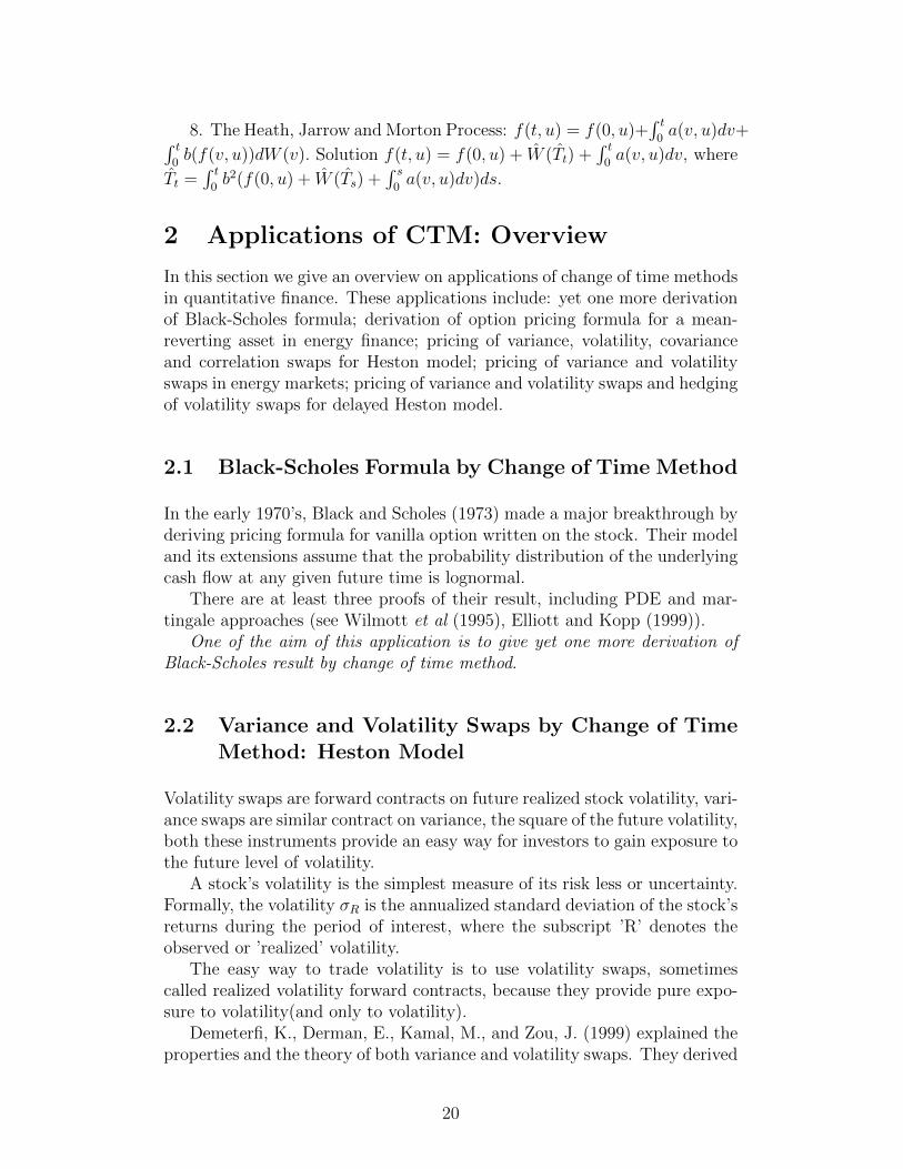
8. The Heath, Jarrow and Morton Process: f(t, u) = f(0, u)+∫ t0a(v, u)dv+∫ t

0b(f(v, u))dW (v). Solution f(t, u) = f(0, u) + W (Tt) +

∫ t0a(v, u)dv, where

Tt =∫ t0b2(f(0, u) + W (Ts) +

∫ s0a(v, u)dv)ds.

2 Applications of CTM: Overview

In this section we give an overview on applications of change of time methodsin quantitative finance. These applications include: yet one more derivationof Black-Scholes formula; derivation of option pricing formula for a mean-reverting asset in energy finance; pricing of variance, volatility, covarianceand correlation swaps for Heston model; pricing of variance and volatilityswaps in energy markets; pricing of variance and volatility swaps and hedgingof volatility swaps for delayed Heston model.

2.1 Black-Scholes Formula by Change of Time Method

In the early 1970’s, Black and Scholes (1973) made a major breakthrough byderiving pricing formula for vanilla option written on the stock. Their modeland its extensions assume that the probability distribution of the underlyingcash flow at any given future time is lognormal.

There are at least three proofs of their result, including PDE and mar-tingale approaches (see Wilmott et al (1995), Elliott and Kopp (1999)).

One of the aim of this application is to give yet one more derivation ofBlack-Scholes result by change of time method.

2.2 Variance and Volatility Swaps by Change of TimeMethod: Heston Model

Volatility swaps are forward contracts on future realized stock volatility, vari-ance swaps are similar contract on variance, the square of the future volatility,both these instruments provide an easy way for investors to gain exposure tothe future level of volatility.

A stock’s volatility is the simplest measure of its risk less or uncertainty.Formally, the volatility σR is the annualized standard deviation of the stock’sreturns during the period of interest, where the subscript ’R’ denotes theobserved or ’realized’ volatility.

The easy way to trade volatility is to use volatility swaps, sometimescalled realized volatility forward contracts, because they provide pure expo-sure to volatility(and only to volatility).

Demeterfi, K., Derman, E., Kamal, M., and Zou, J. (1999) explained theproperties and the theory of both variance and volatility swaps. They derived

20

an analytical formula for theoretical fair value in the presence of realisticvolatility skews, and pointed out that volatility swaps can be replicated bydynamically trading the more straightforward variance swap.

Javaheri A, Wilmott, P. and Haug, E. G. (2002) discussed the valuationand hedging of a GARCH(1,1) stochastic volatility model. They used ageneral and exible PDE approach to determine the first two moments of therealized variance in a continuous or discrete context. Then they approximatethe expected realized volatility via a convexity adjustment.

Brockhaus and Long (2000) provided an analytical approximation forthe valuation of volatility swaps and analyzed other options with volatilityexposure.

Working paper by Theoret, Zabre and Rostan (2002) presented an analyt-ical solution for pricing of volatility swaps, proposed by Javaheri, Wilmottand Haug (2002). They priced the volatility swaps within framework ofGARCH(1,1) stochastic volatility model and applied the analytical solutionto price a swap on volatility of the S&P60 Canada Index (5-year historicalperiod: 1997− 2002).

Although options market participants talk of volatility, it is variance, orvolatility squared, that has more fundamental significance (see Demeterfi,K., Derman, E., Kamal, M., and Zou, J. (1999)).

Modeling and pricing of variance, volatility, covariance and correlationswaps for Heston model have been considered in Swishchuk (2004). In thispaper, a new probabilistic approach, change of time method, was proposedto study variance and volatility swaps for financial markets with underlyingasset and variance that follow the Heston (1993) model. We also studiedcovariance and correlation swaps for the financial markets. As an application,we provided a numerical example using S&P60 Canada Index to price swapon the volatility.

Variance swaps for financial markets with underlying asset and stochas-tic volatilities with delay were modelled and priced in the paper Swishchuk(2005a). We found some analytical close forms for expectation and varianceof the realized continuously sampled variance for stochastic volatility withdelay both in stationary regime and in general case. The key features of thestochastic volatility model with delay are the following: i) continuous-timeanalogue of discrete-time GARCH model; ii) mean-reversion; iii) containsthe same source of randomness as stock price; iv) market is complete; v)incorporates the expectation of log-return. As applications, we provided twonumerical examples using S&P60 Canada Index (1998-2002) and S&P500Index (1990-1993) to price variance swaps with delay. Varinace swaps forstochastic volatility with delay is very similar to variance swaps for stochas-tic volatility in Heston model (see Swishchuk (2004)), but simplier to modeland to price it.

Variance swaps for multi-factor stochastic volatility models with delayhave been studied in Swishchuk (2006).

Pricing of variance swaps in Markov-modulated Brownian markets was

21

considered in Elliott and Swishchuk (2005, 2007).One of the aim of this application is to value variance and volatility swaps

for Heston (1993) model using change of time method.Remark 1.1. A extensive reviews of the literature on stochastic volatility

is given in Shephard (2005a, 2005b). A detailed introduction to variance andvolatility swaps, including a history and market products, may be found inCarr and Madan (1998) and Demeterfi et al (1999). The pricing of a range ofvolatility derivatives, including volatility and variance swaps and swaptions,is studied in Howison et al (2004). This paper also contains a lot of volatilitymodels, including those with jumps. Volatility model with jumps was firstconsidered in Naik (1993). Parameter estimation in a stochastic drift hiddenMarkov model with a cap and with applications to the theory of energyfinance and interest rate modeling is studied in Hernandez et al (2005).

Remark 1.2. The fact that stochastic volatility models, such the Hestonmodel and others, are able to fit skews and smiles, while simultaneouslyproviding sensible Greeks, have made these models a popular choice in thepricing of options and swaps. Some ideas of how to calculate the Greeks forvolatility contracts may be found in Howison et al (2004).

Remark 1.3. We note, that the change of time method was used inSwishchuk and Kalemanova (2000) to study stochastic stability of interestrates with and without jumps, in Swishchuk (2004) to model and to pricevariance and volatility swaps for Heston model and in Swishchuk (2005) toprice European call option for commodity prices that follow mean-revertingmodel.

2.3 Change of Time Method: Delayed Heston Model

Heston model (Heston (1993)) is one of the most popular stochastic volatilitymodels in the industry as semi-closed formulas for vanilla option prices areavailable, few (five) parameters need to be calibrated, and it accounts for themean-reverting feature of the volatility.One might be willing, in the variance diffusion, to take into account notonly its current state but also its past history over some interval [t − τ, t],where τ > 0 is a constant and is called the delay. Starting from the discrete-time GARCH(1,1) model (Bollerslev (1986)), a first attempt was made inthis direction in Kazmerchuk et al. (2005), where a non-Markov delayedcontinuous-time GARCH model was proposed We present a variance driftadjusted version of the Heston model which leads to a significant improve-ment of the market volatility surface fitting by 44% (compared to Heston).The numerical example we performed with recent market data shows a sig-nificant reduction of the average absolute calibration error 1 (calibration on

1The average absolute calibration error is defined to be the average of the absolutevalues of the differences between market and model implied Black & Scholes volatilities.

22

12 dates ranging from Sep. 19th to Oct. 17th 2011 for the FOREX un-derlying EURUSD). Our model has two additional parameters compared tothe Heston model, can be implemented very easily and was initially intro-duced for volatility derivatives pricing purpose. The main idea behind ourmodel is to take into account some past history of the variance process in its(risk-neutral) diffusion. Using a change of time method for continuous localmartingales, we derive a closed formula for the Brockhaus&Long approxi-mation of the volatility swap price in this model. We also consider dynamichedging of volatility swaps using a portfolio of variance swaps.

One of the aim of this application is to get varinace and volatility swapprices using change of time method and to get hedge ration for volatility swapsin the delayed Heston model model.

2.4 Change of Time Method: Multi-factor Levy-basedModels for Pricing of Financial and Energy Deriva-tives

We also introduce one-factor and multi-factor α-stable Levy-based models toprice financial and energy derivatives. These models include, in particular,as one-factor models, the Levy-based geometric motion model, the Ornstein-Uhlenbeck (1930), the Vasicek (1977), the Cox-Ingersoll-Ross (1985), thecontinuous-time GARCH, the Ho-Lee (1986), the Hull-White (1990) andthe Heath-Jarrrow-Morton (1992) models, and, as multi-factor models, var-ious combinations of the previous models. For example, we introduce newmulti-factor models such as the Levy-based Heston model, the Levy-basedSABR/LIBOR market models, and Levy-based Schwartz-Smith and Schwartzmodels. Using the change of time method for SDEs driven by α-stable Levyprocesses we present the solutions of these equations in simple and com-pact forms. We then apply this method to price many financial and energyderivatives such as variance swaps, options, forward and futures contracts.

One of the aim of this application is to consider various applications of thechange of time method for Levy-based SDEs arising in financial and energymarkets: swap and option pricing, interest derivatives pricing and forwardand futures contracts pricing.

2.5 Mean-Reverting Asset Model by Change of TimeMethod: Option Pricing Formula

Some commodity prices, like oil and gas, exhibit the mean reversion, unlikestock price. It means that they tend over time to return to some long-termmean. This mean-reverting model is a one-factor version of the two-factormodel made popular in the context of energy modeling by Pilipovic (1997).

23

Black’s model (1976) and Schwartz’s model (1997) have become a standardapproach to the problem of pricing options on commodities. These modelshave the advantage of mathematical convenience, in that they give rise toclosed-form solutions for some types of option (see Wilmott (2000)).

Bos, Ware and Pavlov (2002) presented a method for evaluation of theprice of a European option based on St using a semi-spectral method. Theydid not have the convenience of a closed-form solution, however, they shownthat values for certain types of option may nevertheless be found extremelyefficiently. They used the following partial differential equation (see, forexample, Wilmott, Howison and Dewynne (1995))

C ′t +R(S, t)C ′S + σ2S2C ′′SS/2 = rC

for option prices C(S, t), where R(S, t) depends only on S and t, and corre-sponds to the drift induced by the risk-neutral measure, and r is the risk-freeinterest rate. Simplifying this equation to the singular diffusion equationthey were able to calculate numerically the solution.

The working paper Swishchuk (2005b) presents explicit expression for aEuropean option price, C(S, t), for mean-reverting asset St, using change oftime method under both physical and risk-neutral measures.

We note, that recent book by Geman (2005) covers hard and soft com-modities (energy, agriculture and metals) and analysis economic and geopo-litical issues in commodities markets, commodity price and volume risk,stochastic modeling of commodity spot prices and forward curves, real op-tions valuation and hedging of physical assets in the energy industry.

One of the aim of this application is to obtain explicit expression for aEuropean call option price on mean-reverting model of commodity asset usingchange of time method. As we can see, if mean-reverting level equals to zerothen the option pricing formula coincides with Black-Scholes result.

2.6 Variance and Volatility Swaps by Change of TimeMethod: Energy Markets

One of applications of CTM is devoted to the pricing of variance and volatil-ity swaps in energy market. We found explicit variance swap formula andclosed form volatility swap formula (using change of time) for energy as-set with stochastic volatility that follows continuous-time mean-revertingGARCH (1,1) model. Numerical example is presented for AECO NaturalGas Index (1 May 1998-30 April 1999). Variance swaps are quite common incommodity, e.g., in energy market, and they are commonly traded. We con-sider Ornstein-Uhlenbeck process for commodity asset with stochastic volatil-ity following continuous-time GARCH model or Pilipovic (1998) one-factormodel. The classical stochastic process for the spot dynamics of commodityprices is given by the Schwartz’ model (1997). It is defined as the exponential

24

of an Ornstein-Uhlenbeck (OU) process, and has become the standard modelfor energy prices possessing mean-reverting features.

In this book, we consider a risky asset in energy market with stochasticvolatility following a mean-reverting stochastic process satisfying the follow-ing SDE (continuous-time GARCH(1,1) model):

dσ2(t) = a(L− σ2(t))dt+ γσ2(t)dWt,

where a is a speed of mean reversion, L is the mean reverting level (orequilibrium level), γ is the volatility of volatility σ(t), Wt is a standard Wienerprocess. Using a change of time method we find an explicit solution of thisequation and using this solution we are able to find the variance and volatilityswaps pricing formula under the physical measure. Then, using the sameargument, we find the option pricing formula under risk-neutral measure. Weapplied Brockhaus-Long (2000) approximation to find the value of volatil;ityswap. A numerical example for the AECO Natural Gas Index for the period1 May 1998 to 30 April 1999 is presented.

Commodities are emerging as an asset class in their own. The range ofproducts offered to investors range from exchange traded funds (ETFs) tosophisticated products including principal protected structured notes on indi-vidual commodities or baskets of commodities and commodity range-accrualor varinace swap. More and more institutional investors are including com-modities in their asset allocation mix and hedge funds are also increasinglyactive players in commodities. Example: Amaranth Advisors lost USD 6billion during September 2006 from trading natural gas futures contracts,leading to the fund’s demise. Concurrent with these developments, a num-ber of recent papers have examined the risk and return characteristics of in-vestments in individual commodity futures or commodity indices composedof baskets of commodity futures. However, since all but the most plain-vanilla investments contain an exposure to volatility, it is equally importantfor investors to understand the risk and return characteristics of commodityvolatilities.

The focusing on energy commodities derives from two reasons: 1) en-ergy is the most important commodity sector, and crude oil and natural gasconstitute the largest components of the two most widely tracked commod-ity indices: the Standard & Poors Goldman Sachs Commodity Index (S&PGSCI) and the Dow Jones-AIG Commodity Index (DJ-AIGCI); 2) existenceof a liquid options market: crude oil and natural gas indeed have the deepestand most liquid options marketss among all commodities. The idea is to usevariance (or volatility) swaps on futures contracts. At maturity, a varianceswap pays off the difference between the realized variance of the futures con-tract over the life of the swap and the fixed variance swap rate. And sincea variance swap has zero net market value at initiation, absence of arbitrageimplies that the fixed variance swap rate equals to conditional risk-neutralexpectation of the realized variance over the life of swap. Therefore, e.g., the

25

time-series average of the payoff and/or excess return on a variance swap isa measure of the variance risk premium.

Variance risk premia in energy commodities, crude oil and natural gas, hasbeen considered by A. Trolle and E. Schwartz (2009). The same methodologyas in Trolle & Schwartz (2009) was used by Carr & Wu (2009) in their studyof equity variance risk premia. The idea was to use variance swaps on futurescontracts. The study in Trolle & Schwartz (2009) is based on daily data fromJanuary 2, 1996 until November 30, 2006-a total of 2750 business days. Thesource of the data is NYMEX. Trolle & Schwartz (2009) found that: 1) theaverage variance risk premia are negative for both energy commodities butmore strongly statistically significant for crude oil than for natural gas; 2)the natural gas variance risk premium (defined in dollars terms or in returnterms) is higher during the cold months of the year (seasonality and peaksfor natural gas variance during the cold months of the year); 3) energy riskpremia in dollar terms are time-varying and correlated with the level of thevariance swap rate. In contrast, energy variance risk premia in return terms,paerticularly in the case of natural gas, are much less correlated with thevarinace swap rate.

The S&P GSCI is comprised of 24 commodities with the weight of eachcommodity determined by their relative levels of world production over thepast five years. The DJ-AIGCI is comprised of 19 commodities with theweight of each component detrmined by liquidity and world production val-ues, with liquidity being the dominant factor. Crude oil and natural gas arethe largest components in both indices. In 2007, their weight were 51.30%and 6.71%, respectively, in the S&P GSCI and 13.88% and 11.03%, respec-tively, in the DJ-AIGCI. The Chicago Board Optiopns Exchange (CBOE)recently introduced a Crude Oil Volatility Index (ticker symbol OVX). Thisindex also measures the conditional risk-neutral expectation of crude oil vari-ance, but is computed from a cross-section of listed options on the UnitedStates Oil Fund (USO), which tracks the price of WTI as closely as possi-ble. The CBOE Crude Oil ETF Volatility Index (’Oil VIX’, Ticker - OVX)measures the market’s expectation of 30-day volatility of crude oil pricesby applying the VIX methodology to United States Oil Fund, LP (Ticker -USO) options spanning a wide range of strike prices. We have to notice thatcrude oil and natural gas trade in units of 1,000 barrels and 10,000 Britishthermal units (mmBtu), respectivel. Price are quoted as US dollars andcents per barrel or mmBtu. The continuous-time GARCH model has alsobeen exploited by Javaheri, Wilmott and Haug (2002) to calculate volatilityswap for S&P500 index. They used PDE approach and mentioned (page 8,sec. 3.3) that ’it would be interesting to use an alternative method to calcu-late F (v, t) and the other above quantities’. This paper exactly contains thealternative method, namely, ’change of time method’, to get varinace andvolatility swaps. The change of time method was also applied by Swishchuk(2004) for pricing variance, volatility, covariance and correlation swaps forHeston model. The first paper on pricing of commodity contracts was pub-

26

lished by Black (1976).One of the aim of this application is to get variance and volatility swap

prices for Heston model using change of time method.

References

Applebaum, D. (2004): Levy Processes and Stochastic Calculus, Cam-bridge University Press.

Barnhoff-Nielsen, O.E. and Shephard, N. (2001): Modelling byLevy processes for financial econometrics, in Levy Processes-Theory and Ap-plications, Birkhauser.

Barndorff-Nielsen O.E., Mikosch, T. and Resnick, S. (eds.) (2001):Levy Processes: Theory and Applications, Birkhauser.

Barndorff-Nielsen O.E., Mikosch, T. and Resnick, S. (eds.) (2001):Levy Processes: Theory and Applications, Birkhauser, pp. 283-718.

Barnhoff-Nielsen, O.E. and Shephard, N. (2002): Econometric anal-ysis of realized volatility andits use in estimating stochastic volatility models,J. R. Statistic Soc. B, 64, pp. 253-280.

Barnhoff-Nielsen, O.E., Nicolato, E. and Shephard, N. (2002):Some recent development in stochastic volatility modeling, Quantitative Fi-nance, 2, 11-23.

Barnhoff-Nielsen, O.E. and Shiryaev A. (2009): Change of Timeand Change of Measure. World Scientific.

Bates, D. (1996): Jumps and stochastic volatility: the exchange rate pro-cesses implicit in Deutschemark options. Rev. Fin. Studies, 9, pp. 69-107.

Bertoin, J. (1996): Levy Processes, Cambridge University Press.

Black, F. and Scholes, M. (1973): The pricing of options and corporateliabilities, J. Political Economy 81, 637-54.

Black, F. (1076): The pricing of commodity contarcts, J. Financial Eco-nomics, 3, 167-179.

Bochner, S. (1949): Diffusion equation and stochastic processes. Proc.Nat. Acad. Sci. USA, 85, 369-370.

Bollerslev, T. (1986): Generalized autoregressive conditional heteroscedas-ticity. Journal of Economics, 31: 307-27.

Bos, L.P., Ware, A. F. and Pavlov, B. S. (2002): On a semi-spectralmethod for pricing an option on a mean-reverting asset, Quantitative Fi-nance, Volume 2, 337-345.

27

Brockhaus, O. and Long, D. (2000): Volatility swaps made simple,RISK, January, 92-96.

Carr, P. and Madan, D. (1998): Towards a Theory of Volatility Trading.In the book: Volatility, Risk book publications,http://www.math.nyu.edu/research/carrp/papers/.

Carr, P., Geman, H., Madan, D. and Yor, M. (2003): Stochasticvolatility for Levy processes, Mathem. Finance, 13, pp. 345-382.

P. Carr and L. Wu (2009): Variance risk premia, Review of FinancialStudies 22, 1311-1341.

Chesney, M. and Scott, L. (1989): Pricing European Currency Op-tions: A comparison of modifeied Black-Scholes model and a random variancemodel, J. Finan. Quantit. Anal. 24, No3, 267-284.

Cherny, A. and Shiryaev, A. (2002): Change of time and change ofmeasure for Levy processes. Lecture Notes 13, Aarhus University, Aarhus,46p.

Clark, P. (1973): A subordinated stochastic process model with fixedvariance for speculative prices, Econometrica, 41, 135-156.

Cont, R. and Tankov, P. (2004): Financial Modeling with Jump Pro-cesses, Chapman & Hall/CRC Fin. Math. Series.

Cox, J., Ingersoll, J. and Ross, S. (1985): A theory of the termstructure of interest rates, Econometrica 53, 385-407.

Dambis, K.E. (1965): On the decomposition of continuous submartingales,Theory Probabability and its Appl., 10, 4091-410.

Dubins and Schwartz (1965): On continuous martingales, Proc. Nat.Acad. Sciences, USA, 53, 913-916.

Demeterfi, K., Derman, E., Kamal, M. and Zou, J. (1999): A guideto volatility and variance swaps, The Journal of Derivatives, Summer, 9-32.

Elliott, R. (1982): Stochastic Calculus and Applications, Springer-Verlag,New York.

Elliott, R. and Kopp, P. (1999): Mathematics of Financial Markets,Springer-Verlag, New York.

Elliott, R. and Swishchuk, A. (2005): Pricing options and volatilityswaps in Markov-modulated Brownian and Fractional Brownian markets,RJE 2005 Conference, Calgary, AB, Canada, July 24-27, 2005, 35p.

Elliott, R. and Swishchuk, A. (2007): Pricing options and variance

28

swaps in Markov-modulated Brownian markets, In: Hidden Markov Mod-els in Finance, Springer, International Series in Operations Research andManagement Science, Eds.: Elliott, R. and Mamon, R.

Feller, W. (1966): Introduction to Probability Theory and its Applica-tions, v. II, Wiley & Sons.

Geman, H., Madan, D. and Yor, M. (2001): Time changes for Levyprocesses, Mathem. Finance, 11, pp. 79-96.

Geman, H., Madan, D. and Yor, M. (2001): Asset prices are Brownianmotion: only in business time, in Quantitative Analysis in Financial Markets,Avellaneda, M., ed., World Scientific: River Edge, NJ, pp. 103-146.

Geman, H. (2005): Commodities and Commodity Derivatives: Modellingand Pricing for Agricaltural, Metals and Energy, Wiley.

D. Heath, R.Jarrow and A.Morton: Bond pricing and the term struc-ture of the interest rates: A new mathodology. Econometrica, 60, 1 (1992),pp. 77-105.

Hernandez,J., Sounders, D. and Seco, L. (2005): Parameter Esti-mations in a Stochastic Drift Hidden Markov Model with a Cap, submittedto SIAM.

Heston, S. (1993): A closed-form solution for options with stochasticvolatility with applications to bond and currency options, Review of Finan-cial Studies, 6, 327-343

Ho T.S.Y. and Lee S.-B.: Term structure movements and pricing interestrate contigent claim. J. of Finance, 41 (December 1986), pp. 1011-1029.

Hobson, D. and Rogers, L. (1998): Complete models with stochasticvolatility, Math. Finance 8, no.1, 27-48.

Howison, S., Rafailidis, A. and Rasmussen, H. (2004): On the Pric-ing and Hedging of Volatility Derivatives, Applied Math. Finance J., p.1-31.

Huff, B. (1969): The loose subordination of differential processes to Brow-nian motion, Ann. Math. Statist., 40, 1603-1609.

Hull, J., and White, A. (1987): The pricing of options on assets withstochastic volatilities, J. Finance 42, 281-300.

Ikeda, N. and Watanabe, S. (1981): Stochastic Differential Equationsand Diffusion Processes, North-Holland/Kodansha Ltd., Tokyo.

Kallsen, J. and Shiryaev, A. (2001): Time change representation ofstochastic integrals. Theory Probab. Appl. 46, 3, 522-528.

Kazmerchuk, Y., Swishchuk, A. and Wu, J. (2005): A continuous-

29

time GARCH model for stochastic volatility with delay. Canadian AppliedMathematics Quarterly, 13, 2: 123-149.

Knight, F. (1971) A reduction of continuous, square-integrable martin-gales to Brownian motion, in: H. Dinges, ed., Martingales, Lecture Notes inMath. No. 190 (Springer, Berlin) pp. 19-31.

Javaheri, A., Wilmott, P. and Haug, E. (2002): GARCH and volatil-ity swaps, Wilmott Technical Article, January, 17p.

Lamperton, D. and Lapeyre, B. (1996): Introduction to StochasticCalculus Applied to Finance, Chapmann & Hall.

Liptser R. and Shiryaev A. (1989): Theory of Martingales. Kluwer,Dordrecht.

Liptser R. and Shiryaev A. (2001): Statistics of Random Processes.Vol. I: General Theory; Vol. II: Applications, 2nd edn. Springer-Verlag,Berlin.

Madan, D. and Seneta, E. (1990): The variance gamma (VG) modelfor share market returns, Journal of Business 63, No. 4, 511-524.

Merton, R. (1973): Theory of rational option pricing, Bell Journal ofEconomic Management Science 4, 141-183.

Monroe, I. (1972): On embedding right continuous martingales in Brow-nian motion, Ann. Math. Statist., 43, 1293-1311.

Monroe, I. (1978): Processes that can be embedded in Brownian motion,The Annals of Probab., 6, No. 1, 42-56.

Naik, V. (1993): Option Valuation and Hedging Strategies with Jumps inthe Volatility of Asset Returns, Journal of Finance, 48, 1969-84.

Øksendal, B. (1998): Stochastic Differential Equations: An Introductionwith Applications. NY: Springer.

Pilipovic, D. (1997): Valuing and Managing Energy Derivatives, NewYork, McGraw-Hill.

Price Pseudo-Variance, Pseudo-Covariance, Pseudo-Volatility, and Pseudo-Correlation Swaps-In Analytical Closed-Forms, Proceedings of the Sixth PIMSIndustrial Problems Solving Workshop, PIMS IPSW 6, University of BritishColumbia, Vancouver, Canada, May 27-31, 2002, pp. 45-55. Editor: J.Macki, University of Alberta, June 2002. (Joint report: Raymond Cheng,Stephen Lawi, Anatoliy Swishchuk, Andrei Badescu, HammoudaBen Mekki, Asrat Fikre Gashaw, Yuanyuan Hua, Marat Moly-boga, Tereza Neocleous, Yuri Petrachenko).

30

Schoutens, W. (2003): Levy Processes in Finance: Pricing Derivatives,Wiley.

Shephard, N. (2005a): Stochastic Volatility: Selected Readings. Oxford:Oxford University Press.

Shephard, N. (2005b): Stochastic Volatility. Working paper, Univresityof Oxford, Oxford.

Skorokhod, A. (1965): Studies in the Theory of Random Processes,Addison-Wesley, Reading.

Schwartz, E. (1997): The stochastic behaviour of commodity prices: im-plications for pricing and hedging, J. Finance, 52, 923-973.

Swishchuk, A. and Kalemanova, A. (2000): Stochastic stability ofinterest rates with jumps. Theory probab. & Mathem statist., TBiMC Sci.Publ., v.61, Kiev, Ukraine.

Swishchuk, A. (2004): Modeling and valuing of variance and volatilityswaps for financial markets with stochastic volatilities, Wilmott Magazine,Technical Article No2, September Issue, 64-72.

Swishchuk, A. (2005a): Modelling and Pricing of Variance Swaps forStochastic Volatilities with Delay, Wilmott Magazine, Technical Article, Septem-ber Issue (to appear).

Swishchuk, A. (2008): Explicit option pricing formula for mean-revertingmodel, J. Numer. Appl. Math., Vol. 1(96), 2008, pp.216-233.

Swishchuk, A. (2006): Modelling and pricing of variance swaps for multi-factor stochastic volatilities with delay, Canadian Applied Math. Quarterly,14, No. 4, Winter.

Theoret, R., Zabre, L. and Rostan, P. (2002): Pricing volatilityswaps: empirical testing with Canadian data. Working paper, Centre deRecherche en Gestion, Document 17-2002, July 2002.

Trolle, A. and Schwartz, E. (2010): Variance risk premia in energycommodities, J. of Derivatives, Spring, v. 17, No. 3, 15-32.

Wilmott, P., Howison, S. and Dewynne, J. (1995): Option Pricing:Mathematical Models and Computations. Oxford: Oxford Financial Press.

Wilmott, P., Howison, S. and Dewynne, J. (1995): The Mathematicsof Financial Derivatives, Cambridge, Cambridge University Press.

Wilmott, P. (2000): Paul Wilmott on Quantitative Finance, New York,Wiley.

Winkel, M. (2001): The recovery problem for time-changed Levy pro-

31

cesses, Res. Report, 2001-37, MaPhySto, October.

32

Chapter 3: Change of Time Method (CTM)

and Black-Scholes Formula

’It is said that there is no such thing as a free lunch. But the universe is theultimate free lunch’,-Alan Guth (MIT).

1 Introduction to Option Pricing and Black-

Scholes Formula

In this Chapter, we consider applications of the change of time method toyet one more time derive the well-known Black-Scholes formula for Europeancall options. In the early 1970’s, Black and Scholes, (1973), made a majorbreakthrough by deriving a pricing formula for a vanilla option written onthe stock. Their model and its extensions assume that the probability distri-bution of the underlying cash flow at any given future time is lognormal. Wemention that there are many proofs of this result, including PDE and martin-gale approaches, (see Wilmott et. al. (1995), Elliott and Kopp (1999)). Thepresent approach, using change of time of getting the Black-Scholes formulawas first shown in Swishchuk (2007).

1.1 A Brief and Quick Introduction to Option PricingTheory

We use the term asset to describe any financial object whose value is knownat present but is liable to change in the future. Some examples include sharesof a company, commodities (oil, electicity, gas, gold, etc.), currencies. etc.Now we give the definitions of options.

Definition 1 (European Call Option). A European call option givesits holder the right (but not the obligation) to purchase from the writer aprescribed asset for a prescribed price at a prescribed time in the future.

Definition 2 (European Put Option). A European call option givesits holder the right (but not the obligation) to sell to the writer a prescribedasset for a prescribed price at a prescribed time in the future.

The prescribed purchase price is known as the exercise price or strikeprice, and the prescribed time in the future is known as the expiry date ormaturity. The key question in option pricing theory is: how much should theholder pay for the privilege of holding an option? Or, how do we compute afair option price or value?

Let (Ω,F ,Ft, P ) be a filtered probability space, t ∈ [0, T ], and FT = F .We denote by T the expiry date, by K the strike price and by S(t) the assetprice at time t ≥ 0. Then, e.g., S(T ) is the asset price at the expiry date,which is not known (uncertain or random) at the time when the option istaken out. If S(T ) > K at expiry T, then the holder of a European call

33

option may buy the asset for K and sell it in the market for S(T ), gainingan amount S(T )−K. If K ≥ S(T ), on the other hand, then the holder gainsnothing or zero. Therefore, the value or price of the European call option atthe expiry date, denoted by C(T ), is

fC(T ) = maxS(T )−K, 0.

As for a European put option, the situation is opposite. If S(T ) < K atexpiry T, then the holder of a European put option may buy the asset forS(T ) in the market and sell it in the market for K, gaining an amountK−S(T ). If K ≤ S(T ), on the other hand, then the holder gains nothing orzero. Therefore, the value or price of the European put option at the expirydate, denoted by P (T ), is

fP (T ) = maxK − S(T ), 0.

We call fC(T ) and fP (T ) the payoff functions. The shapes of the correspond-ing paoyff diagrams look like (ice) hockey sticks with the kinks at K.

European call and put options are the simplest and classical examples ofso-called financial derivatives, meaning those derivatives indicate that theirvalues is derived from the underlying asset (do not mix up this term withthe mathematical meaning of a derivative!). There are many other financialderivatives, such as forwards, futures, swaps, etc.

Next question in option pricing theory is: how to determine a fair value orprice of the option at time t = 0? We denote this value or price (for Europeancall option) by C(0). To answer this question we introduce two key concepts:discounting for interest and the no arbitrage principle (sometimes referred toas no free lunch opportunity).

Discounting interest: If we have some money in a risk-free savings aco-cunt (bank deposit) and this investment grows accordingly to a continuouslycompounded interest rate r > 0, then its value increases by a factor ert overa time length t. We will use r to denote the annual rate (so that time is mea-sured in years). The simplest example is risk-free bank account with amountof money B(t) at time t > 0. If the intiial deposit is B(0), then at time t > 0it will be B(t) = ertB(0). Hence, B(t) satisfies the equation dB(t) = rB(t)dt,B(0) > 0, r > 0, t ≥ 0. Suppose also that we have an amount C(0) at timetime zero, then it is worth C(t) = ertC(0) at time t or C(T ) = erTC(0) atexpiry T. It means that to have C(T ) amount of money on saving account attime T we have to have C(0) = e−rTC(T ) amount of money at time t = 0.

No Arbitrage Principle: This principle means that there is never an op-portunity to make a risk-free profit that gives a greater return than thatprovided by the interest from bank deposit. Arguments based on the NoArbirage principle are the main tools of financial mathematics.

The key role for criteria of No Arbitrage plays the problem of changeof measures which is crucial in mathematical finance. We call this measure” martingale measure” or ”risk-neutral measure”, and denote it by Q, to

34

make it different from the initial or physical probability measure P. Thetechnic of change of measure is based on the construction of a new probabilitymeasure Q equivalent to the given measure P and such that a process S(t),built on initial process S(t) satisfies some ’fairness’ condition. In the caseof mathematical finance, this process S(t) = e−rtS(t) is a martingale withrespect to the new measure Q. As long as asset value S(t) at time t is randomor unknown, we have to calculate the expected value of this asset. It meansthat expectation should be taking with repsect to this martingale measureQ. Returning to our payoff functions, it means that we have to calculatethis expected value (we denote it by EQ, compare with EP -expectation withrespect to the initial measure P ) with respect to the risk-neutral measureQ : EQ[maxS(T )−K, 0].

Therefore, if the initial (at time t = 0) fair price of option is C(0), thenthe value EQ[maxS(T )−K] is equal to erTC(0) or

C(0) = e−rTEQ[maxS(T )−K, 0]. (∗)

This formulae gives the answer to our question: the fair price of the optionat time t = 0 is defined by the last formulae.

The situation for the European put option is similar, taking into accountthe payoff function P (T ) = maxK − S(T ), 0 in this case. Therefore, thefair price P (0) of the European put option at time t = 0 is

P (0) = e−rTEQ[maxK − S(T ), 0].

We note, that fair prices of European call and put options satisfy the followingso-called call-put parity:

C(0) +Ke−rT = P (0) + S(0),

where S(0) is the iniiial (at time t = 0) asset price. See Elliott et al. (1999)or Wilmott et al. (1995) for more details on option pricing.

1.2 Black-Scholes Formula

The well-known Black-Scholes (1973) formula states that if we have a(B, S)-security market consisting of a riskless asset B(t) with a constantcontinuously compounded interest rate r :

dB(t) = rB(t)dt, B(0) > 0, r > 0. (1)

The risky asset, (stock), S(t) is assumed to have dynamics

dS(t) = µS(t)dt+ σS(t)dW (t), S(0) > 0. (2)

Here: µ ∈ R is the appreciation rate and σ > 0 is the volatility. Then pricefor a European call option with pay-off function f(T ) = max(S(T ) −K, 0),(K > 0 is the strike price), has the following form:

35

C(T ) = S(0)Φ(y+)− e−rTKΦ(y−), (3)

where

y± :=ln(S(0)

K) + (r ± σ2

2)T

σ√T

(4)

and

Φ(y) :=1√2π

∫ y

−∞e−

x2

2 dx. (5)

1.3 Solution of SDE for Geometric Brownian Motionusing Change of Time Method

Lemma 1. The solution of the equation (3.2) has the following form:

S(t) = eµt(S(0) + W (φ−1s )), (6)

where W (t) is a one-dimensional Wiener process,

φ−1t = σ2

∫ t

0

[S(0) + W (φ−1s )]2ds

and

φt = σ−2∫ t

0

[S(0) + W (s)]−2ds.

Proof.Set

V (t) = e−µtS(t), (7)

where S(t) is defined in (2).Applying Ito′s formula to V (t) we obtain

dV (t) = σV (t)dW (t). (8)

Equation (8) is similar to equation (9) of Chapter 2, with

a(X) = σX.

Therefore, the solution of equation (3.8) using the change of time method(see Corollary 2.1, Section 2.4, Chapter 2) is (see (10) and (11))

V (t) = S(0) + W (φ−1t ), (9)

where W (t) is an one-dimensional Wiener process,

φ−1t = σ2

∫ t

0

[S(0) + W (φ−1s )]2ds

and

φt = σ−2∫ t

0

[S(0) + W (s)]−2ds.

From (7) and (9) it follows that the solution of equation (2) has therepresentation (6).

36

1.4 Properties of the Process W (φ−1t )

Lemma 2. Process W (φ−1t ) is a mean-zero martingale with quadratic vari-ation

< W (φ−1t ) >= φ−1t = σ2

∫ t

0

[S(0) + W (φ−1s )]2ds

and has the following representation

W (φ−1t ) = S(0)(eσW (t)−σ2

2t − 1). (10)

Proof.From Corollary 2.1, Section 2.4, Chapter 2, it follows that W (φ−1t ) is a

martingale with quadratic variation

< W (φ−1t ) >= φ−1t = σ2

∫ t

0

[S(0) + W (φ−1s )]2ds.

and the process W (t) has the following look

W (t) = σ−1∫ t

0

[S(0) + W (φ−1s ))]−1dW (φ−1s ) (11)

From (11) we obtain the following SDE for W (φ−1s )

dW (φ−1s ) = σ[S(0) + W (φ−1s )]dW (t).

Solving this equation we have the explicit expression (3.10) for W (φ−1s )

W (φ−1s ) = S(0)(eσW (t)−σ2

2t − 1).

Q.E.DWe note that EW (φ−1s ) = 0 and E[W (φ−1t )]2 = S2(0)(eσ

2t − 1), whereE := EP is an expectation under physical measure P.

Since

E[eσW (t)−σ2

2t]n = e

σ2

2n(n−1)t, (12)

we can obtain all the moments for the process W (φ−1s ) :

E[W (φ−1t )]n = Sn(0)n∑k=0

Ckne

σ2t2k(k−1)(−1)n−k, (13)

where Ckn := n!

k!(n−k)! , n! := 1× 2× 3...× n.Corollary 1. From Lemma 2 (see (6), (10) and (12)) it follows that we

can also obtain all the moment for the asset price S(t) in (9), sin

E[S(t)]n = enµtE[S(0) + W (φ−1s )]n

= enµtSn(0)E[eσW (t)−σ2t2 ]n

= enµtSn(0)eσ2

2n(n−1)t.

(14)

37

For example, variance of S(t) is going to be

V arS(t) = ES2(t)− (ES(t))2 = S2(0)e2µt(eσ2t − 1),

where ES(t) = S(0)eµt (see (9)).

2 Black-Scholes Formula by Change of Time

Method

In risk-neutral world the dynamic of stock price S(t) has the following look:

dS(t) = rS(t)dt+ σS(t)dW ∗(t), (15)

where

W ∗(t) := W (t) +µ− rσ

. (16)

Following Section 3.2, from (6) we have the solution of the equation (15)

S(t) = ert[S(0) + W ∗(φ−1t )], (17)

where

(3.18) W ∗(φ−1t ) = S(0)(eσW∗(t)−σ

2t2 − 1)

and W ∗(t) is defined in (16).Let EQ be an expectation under risk-neutral measure (or martingale mea-

sure) Q (i.e., process e−rTS(t) is a martingale under the measure Q).Then the option pricing formula for European call option with pay-off

functionfC(T ) = max[S(T )−K, 0]

has the following look

C(T ) = e−rTEQ[f(T )] = e−rTEP ∗ [max(S(T )−K, 0)]. (19)

Proposition 3.1.

C(T ) = S(0)Φ(y+)−Ke−rTΦ(y−), (20)

where y± and Φ(y) are defined in (4) and (5).Proof. Using change of time method we have the following representation

for the process S(t) (see (17))

S(t) = ert[S(0) + W ∗(φ−1t )],

38

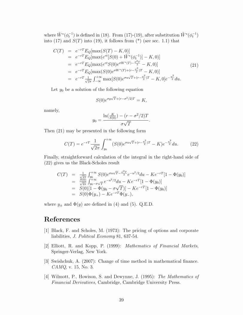
where W ∗(φ−1t ) is defined in (18). From (17)-(19), after substitution W ∗(φ−1t )into (17) and S(T ) into (19), it follows from (*) (see sec. 1.1) that

C(T ) = e−rTEQ[max(S(T )−K, 0)]

= e−rTEQ[max(ert[S(0) + W ∗(φ−1t )]−K, 0)]

= e−rTEQ[max(ertS(0)eσW∗(T )−σ

2T2 −K, 0)]

= e−rTEQ[max(S(0)eσW∗(T )+(r−σ

2

2)T −K, 0)]

= e−rT 1√2π

∫ +∞−∞ max[S(0)eσu

√T+(r−σ

2

2)T −K, 0]e−

u2

2 du.

(21)

Let y0 be a solution of the following equation

S(0)eσy√T+(r−σ2/2)T = K,

namely,

y0 =ln( K

S(0))− (r − σ2/2)T

σ√T

.

Then (21) may be presented in the following form

C(T ) = e−rT1√2π

∫ +∞

y0

(S(0)eσu√T+(r−σ

2

2)T −K)e−

u2

2 du. (22)

Finally, straightforward calculation of the integral in the right-hand side of(22) gives us the Black-Scholes result

C(T ) = 1√2π

∫ +∞y0

S(0)eσu√T−σ

2T2 e−u

2/2du−Ke−rT [1− Φ(y0)]

= S(0)√2π

∫ +∞y0−σ

√Te−u

2/2du−Ke−rT [1− Φ(y0)]

= S(0)[1− Φ(y0 − σ√T )]−Ke−rT [1− Φ(y0)]

= S(0)Φ(y+)−Ke−rTΦ(y−),

where y± and Φ(y) are defined in (4) and (5). Q.E.D.

References

[1] Black, F. and Scholes, M. (1973): The pricing of options and corporateliabilities, J. Political Economy 81, 637-54.

[2] Elliott, R. and Kopp, P. (1999): Mathematics of Financial Markets,Springer-Verlag, New York.

[3] Swishchuk, A. (2007): Change of time method in mathematical finance.CAMQ, v. 15, No. 3.

[4] Wilmott, P., Howison, S. and Dewynne, J. (1995): The Mathematics ofFinancial Derivatives, Cambridge, Cambridge University Press.

39

Chapter 4: CTM and Variance, Volatility, Co-

variance and Correlation Swaps for Classical

Heston Model

’Criticism is easy; achievement is difficult,’-Winston Churchill.

1 Introduction.

In this Chapter, we use CTM to price variance and volatility swaps for fi-nancial markets with underlying asset and variance that follow the classicalHeston (1993) model. We also find covariance and correlation swaps for themodel. As an application, we provide a numerical example using S&P60Canada Index to price swap on the volatility.

In the early 1970’s, Black and Scholes (1973) made a major breakthroughby deriving pricing formulas for vanilla options written on the stock. TheBlack-Scholes model assumes that the volatility term is a constant. Thisassumption is not always satisfied by real-life options as the probability dis-tribution of an equity has a fatter left tail and thinner right tail than thelognormal distribution (see Hull (2000)), and the assumption of constantvolatility σ in financial model (such as the original Black-Scholes model) isincompatible with derivatives prices observed in the market.

The above issues have been addressed and studied in several ways, suchas:(i) Volatility is assumed to be a deterministic function of the time: σ ≡ σ(t)(see Wilmott et al. (1995)); Merton (1973) extended the term structureof volatility to σ := σt (deterministic function of time), with the implied

volatility for an option of maturity T given by σ2T = 1

T

∫ T0σ2udu;

(ii) Volatility is assumed to be a function of the time and the current levelof the stock price S(t): σ ≡ σ(t, S(t)) (see Hull (2000)); the dynamics of thestock price satisfies the following stochastic differential equation:

dS(t) = µS(t)dt+ σ(t, S(t))S(t)dW1(t),

where W1(t) is a standard Wiener process;(iii) The time variation of the volatility involves an additional source of ran-domness, besides W1(t), represented by W2(t), and is given by

dσ(t) = a(t, σ(t))dt+ b(t, σ(t))dW2(t),

where W2(t) and W1(t) (the initial Wiener process that governs the priceprocess) may be correlated (see Buff (2002), Hull and White (1987), Heston(1993));

40

(iv) The volatility depends on a random parameter x such as σ(t) ≡ σ(x(t)),where x(t) is some random process (see Elliott and Swishchuk (2002), Griegoand Swishchuk (2000), Swishchuk (1995), Swishchuk (2000), Swishchuk et al.(2000));(v) Another approach is connected with stochastic volatility, namely, un-certain volatility scenario (see Buff (2002)). This approach is based on theuncertain volatility model developed in Avellaneda et al. (1995), where aconcrete volatility surface is selected among a candidate set of volatility sur-faces. This approach addresses the sensitivity question by computing anupper bound for the value of the portfolio under arbitrary candidate volatil-ity, and this is achieved by choosing the local volatility σ(t, S(t)) among twoextreme values σmin and σmax such that the value of the portfolio is maximizedlocally;

(vi) The volatility σ(t, St) depends on St := S(t + θ) for θ ∈ [−τ, 0],namely, stochastic volatility with delay (see Kazmerchuk, Swishchuk andWu (2002));

In the approach (i), the volatility coefficient is independent of the cur-rent level of the underlying stochastic process S(t). This is a deterministicvolatility model, and the special case where σ is a constant reduces to thewell-known Black-Scholes model that suggests changes in stock prices arelognormal distributed. But the empirical test by Bollerslev (1986) seems toindicate otherwise. One explanation for this problem of a lognormal modelis the possibility that the variance of log(S(t)/S(t − 1)) changes randomly.This motivated the work of Chesney and Scott (1989), where the prices areanalyzed for European options using the modified Black-Scholes model offoreign currency options and a random variance model. In their works theresults of Hull and White (1987), Scott (1987) and Wiggins (1987) were usedin order to incorporate randomly changing variance rates.

In the approach (ii), several ways have been developed to derive thecorresponding Black-Scholes formula: one can obtain the formula by usingstochastic calculus and, in particular, the Ito’s formula (see Øksendal (1998),for example).

A generalized volatility coefficient of the form σ(t, S(t)) is said to belevel-dependent. Because volatility and asset price are perfectly correlated,we have only one source of randomness given by W1(t). A time and level-dependent volatility coefficient makes the arithmetic more challenging andusually precludes the existence of a closed-form solution. However, the ar-bitrage argument based on portfolio replication and a completeness of themarket remain unchanged.

The situation becomes different if the volatility is influenced by a second“non-tradable” source of randomness. This is addressed in the approach(iii), (iv) and (v) we usually obtains a stochastic volatility model, which isgeneral enough to include the deterministic model as a special case. Theconcept of stochastic volatility was introduced by Hull and White (1987),and subsequent development includes the work of Wiggins (1987), Johnson

41

and Shanno (1987), Scott (1987), Stein and Stein (1991) and Heston (1993).We also refer to Frey (1997) for an excellent survey on level-dependent andstochastic volatility models. We should mention that the approach (iv) istaken by, for example, Griego and Swishchuk (2000).

Hobson and Rogers (1998) suggested a new class of non-constant volatilitymodels, which can be extended to include the aforementioned level-dependentmodel and share many characteristics with the stochastic volatility model.The volatility is non-constant and can be regarded as an endogenous factorin the sense that it is defined in terms of the past behaviour of the stockprice. This is done in such a way that the price and volatility form a multi-dimensional Markov process. Volatility swaps are forward contracts on futurerealized stock volatility, variance swaps are similar contract on variance, thesquare of the future volatility, both these instruments provide an easy wayfor investors to gain exposure to the future level of volatility.

A stock’s volatility is the simplest measure of its risk less or uncertainty.Formally, the volatility σR is the annualized standard deviation of the stock’sreturns during the period of interest, where the subscript R denotes theobserved or ”realized” volatility.

The easy way to trade volatility is to use volatility swaps, sometimescalled realized volatility forward contracts, because they provide pure expo-sure to volatility(and only to volatility).

Demeterfi, K., Derman, E., Kamal, M., and Zou, J. (1999) explained theproperties and the theory of both variance and volatility swaps. They derivedan analytical formula for theoretical fair value in the presence of realisticvilatility skews, and pointed out that volatility swaps can be replicated bydynamically trading the more straightforward variance swap.

Javaheri A, Wilmott, P. and Haug, E. G. (2002) discussed the valuationand hedging of a GARCH(1,1) stochastic volatility model. They used ageneral and exible PDE approach to determine the first two moments of therealized variance in a continuous or discrete context. Then they approximatethe expected realized volatility via a convexity adjustment.

Brockhaus and Long (2000) provided an analytical approximation forthe valuation of volatility swaps and analyzed other options with volatilityexposure.

Working paper by Theoret, Zabre and Rostan (2002) presented an analyt-ical solution for pricing of volatility swaps, proposed by Javaheri, Wilmottand Haug (2002). They priced the volatility swaps within framework ofGARCH(1,1) stochastic volatility model and applied the analytical solutionto price a swap on volatility of the S&P60 Canada Index (5-year historicalperiod: 1997− 2002).

In the paper we propose a new probabilistic approach to the study ofstochastic volatility model (Section 3), Heston (1993) model, to model vari-ance and volatility swaps (Section 2). The Heston asset process has a vari-ance σ2

t that follows a Cox, Ingersoll & Ross (1985) process. We find someanalytical close forms for expectation and variance of the realized both con-

42

tinuously (Section 3.4) and discrete sampled variance (Section 3.5), whichare needed for study of variance and volatility swaps, and price of pseudo-variance, pseudo-volatility, the problems proposed by He & Wang (2002) forfinancial markets with deterministic volatility as a function of time. This ap-proach was first applied to the study of stochastic stability of Cox-Ingersoll-Ross process in Swishchuk and Kalemanova (2000).

The same expressions for E[V ] and for V ar[V ] (like in present paper)were obtained by Brockhaus & Long (2000) using another analytical ap-proach. Most articles on volatility products focus on the relatively straight-forward variance swaps. They take the subject further with a simple modelof volatility swaps.

We also study covariance and correlation swaps for the securities marketswith two underlying assets with stochastic volatilities (Section 4).

As an application of our analytical solutions, we provid a numerical ex-ample using S&P60 Canada Index to price swap on the volatility (Section5).

2 Variance and Volatility Swaps.

Volatility swaps are forward contracts on future realized stock volatility, vari-ance swaps are similar contract on variance, the square of the future volatility,both these instruments provide an easy way for investors to gain exposure tothe future level of volatility.

A stock’s volatility is the simplest measure of its risk less or uncertainty.Formally, the volatility σR(S) is the annualized standard deviation of thestock’s returns during the period of interest, where the subscript R denotesthe observed or ”realized” volatility for the stock S.

The easy way to trade volatility is to use volatility swaps, sometimescalled realized volatility forward contracts, because they provide pure expo-sure to volatility (and only to volatility) (see Demeterfi, K., Derman, E.,Kamal, M., and Zou, J. (1999)).

A stock volatility swap is a forward contract on the annualized volatility.Its payoff at expiration is equal to

N(σR(S)−Kvol),

where σR(S) is the realized stock volatility (quoted in annual terms) overthe life of contract,

σR(S) :=

√1

T

∫ T

0

σ2sds,

σt is a stochastic stock volatility, Kvol is the annualized volatility deliveryprice, and N is the notional amount of the swap in dollar per annualizedvolatility point. The holder of a volatility swap at expiration receives Ndollars for every point by which the stock’s realized volatility σR has exceeded

43

the volatility delivery price Kvol. The holder is swapping a fixed volatilityKvol for the actual (floating) future volatility σR. We note that usuallyN = αI, where α is a converting parameter such as 1 per volatility-square,and I is a long-short index (+1 for long and -1 for short).

Although options market participants talk of volatility, it is variance, orvolatility squared, that has more fundamental significance (see Demeterfi,K., Derman, E., Kamal, M., and Zou, J. (1999)).

A variance swap is a forward contract on annualized variance, the squareof the realized volatility. Its payoff at expiration is equal to

N(σ2R(S)−Kvar),

where σ2R(S) is the realized stock variance(quoted in annual terms) over the

life of the contract,

σ2R(S) :=

1

T

∫ T

0

σ2sds,

Kvar is the delivery price for variance, and N is the notional amount ofthe swap in dollars per annualized volatility point squared. The holder ofvariance swap at expiration receives N dollars for every point by which thestock’s realized variance σ2

R(S) has exceeded the variance delivery price Kvar.Therefore, pricing the variance swap reduces to calculating the realized

volatility square.Valuing a variance forward contract or swap is no different from valuing

any other derivative security. The value of a forward contract P on futurerealized variance with strike price Kvar is the expected present value of thefuture payoff in the risk-neutral world:

P = Ee−rT (σ2R(S)−Kvar),

where r is the risk-free discount rate corresponding to the expiration date T,and E denotes the expectation.

Thus, for calculating variance swaps we need to know only Eσ2R(S),

namely, mean value of the underlying variance.To calculate volatility swaps we need more. From Brockhaus-Long (2000)

approximation (which is used the second order Taylor expansion for function√x) we have (see also Javaheri et al (2002), p.16):

E√σ2R(S) ≈

√EV − V arV

8EV 3/2,

where V := σ2R(S) and V arV

8EV 3/2 is the convexity adjustment.

Thus, to calculate volatility swaps we need both EV and V arV .The realised continuously sampled variance is defined in the following

way:

V := V ar(S) :=1

T

∫ T

0

σ2t dt.

44

The realised discrete sampled variance is defined as follows:

V arn(S) :=n

(n− 1)T

n∑i=1

log2 StiSti−1

,

where we neglected by 1n

∑ni=1 log

Sti

Sti−1since we assume that the mean of the

returns is of the order 1n

and can be neglected. The scaling by nT

ensures thatthese quantities annualized (daily) if the maturity T is expressed in years(days).

V arn(S) is unbiased variance estimation for σt. It can be shown that (seeBrockhaus & Long (2000))

V := V ar(S) = limn→+∞

V arn(S).

Realised discrete sampled volatility is given by:

V oln(S) :=√V arn(S).

Realised continuously sampled volatility is defined as follows:

V ol(S) :=√V ar(S) =

√V .

The expressions for V, V arn(S) and V ol(S) are used for calculation of vari-ance and volatility swaps.

3 Variance and Volatility Swaps for Heston

Model of Securities Markets

3.1 Stochastic Volatility Model.

Let (Ω,F ,Ft, P ) be probability space with filtration Ft, t ∈ [0, T ].Assume that underlying asset St in the risk-neutral world and variance

follow the following model, Heston (1993) model:dSt

St= rtdt+ σtdw

1t

dσ2t = k(θ2 − σ2

t )dt+ γσtdw2t ,

(1)

where rt is deterministic interest rate, σ0 and θ are short and long volatility,k > 0 is a reversion speed, γ > 0 is a volatility (of volatility) parameter, w1

t

and w2t are independent standard Wiener processes.

The Heston asset process has a variance σ2t that follows Cox-Ingersoll-

Ross (1985) process, described by the second equation in (1).If the volatility σt follows Ornstein-Uhlenbeck process (see, for example,

Øksendal (1998)), then Ito’s lemma shows that the variance σ2t follows the

process described exactly by the second equation in (1).

45

3.2 Explicit expression for σ2t .

In this section we propose a new probabilistic approach to solve the equationfor variance σ2

t in (1) explicitly, using change of time method (see Ikeda andWatanabe (1981)).

Define the following process:

vt := ekt(σ2t − θ2). (2)

Then, using Ito formula (see Øksendal (1995)) we obtain the equation forvt :

dvt = γekt√e−ktvt + θ2dw2

t . (3)

Using change of time approach to the general equation (see Ikeda andWatanabe (1981))

dXt = α(t,Xt)dw2t ,

we obtain the following solution of the equation (3):

vt = σ20 − θ2 + w2(φ−1t ),

or (see (2)),σ2t = e−kt(σ2

0 − θ2 + w2(φ−1t )) + θ2, (4)

where w2(t) is an Ft-measurable one-dimensional Wiener process, φ−1t is aninverse function to φt:

φt = γ−2∫ t

0

ekφs(σ20 − θ2 + w2(t)) + θ2e2kφs−1ds.

3.3 Properties of processes w2(φ−1t ) and σ2t .

The properties of w2(φ−1t ) := b(t) are the following:

Eb(t) = 0; (5)

E(b(t))2 = γ2ekt − 1

k(σ2

0 − θ2) +e2kt − 1

2kθ2; (6)

Eb(t)b(s) = γ2ek(t∧s) − 1

k(σ2

0 − θ2) +e2k(t∧s) − 1

2kθ2, (7)

where t ∧ s := min(t, s).Using representation (4) and properties (5)-(7) of b(t) we obtain the prop-

erties of σ2t . Straightforward calculations give us the following results:

Eσ2t = e−kt(σ2

0 − θ2) + θ2;

Eσ2t σ

2s = γ2e−k(t+s) ek(t∧s)−1

k(σ2

0 − θ2)

+ e2k(t∧s)−12k

θ2+ e−k(t+s)(σ20 − θ2)2

+ e−kt(σ20 − θ2)θ2 + e−ks(σ2

0 − θ2)θ2 + θ4.

(8)

46

3.4 Valuing Variance and Volatility Swaps

From formula (8) we obtain mean value for V :

EV = 1T

∫ T0Eσ2

t dt

= 1T

∫ T0e−kt(σ2

0 − θ2) + θ2dt

= 1−e−kT

kT(σ2

0 − θ2) + θ2.

(9)

The same expression for E[V ] may be found in Brockhaus and Long(2000).

Substituting E[V ] from (9) into formula

P = e−rT (Eσ2R(S) −Kvar) (10)

we obtain the value of the variance swap.Variance for V equals to:

V ar(V ) = EV 2 − (EV )2.

From (9) we have:

(EV )2 =1− 2e−kT + e−2kT

k2T 2(σ2

0 − θ2)2 +2(1− e−kT )

kT(σ2

0 − θ2)θ2 + θ4. (11)

Second moment may found as follows using formula (8):

EV 2 = 1T 2

∫ T0

∫ T0Eσ2

t σ2sdtds

= γ2

T 2

∫ T0

∫ T0e−k(t+s) ek(t∧s)−1

k(σ2

0 − θ2) + e2k(t∧s)−12k

θ2dtds

+ 1−2e−kT+e−2kT

k2T 2 (σ20 − θ2)2 + 2(1−e−kT )

kT(σ2

0 − θ2)θ2 + θ4.

(12)

Taking into account (11) and (12) we obtain:

V ar(V ) = EV 2 − (EV )2

= γ2

T 2

∫ T0

∫ T0e−k(t+s) ek(t∧s)−1

k(σ2

0 − θ2) + e2k(t∧s)−12k

θ2dtds.

After calculations the last expression we obtain the following expression forvariance of V :

V ar(V ) = γ2e−2kT

2k3T 2 [(2e2kT − 4ekTkT − 2)(σ20 − θ2)

+ (2e2kTkT − 3e2kT + 4ekT − 1)θ2].(13)

47

Similar expression for V ar[V ] may be found in Brockhaus and Long(2000).

Substituting EV from (9) and V ar(V ) from (13) into formula

P = e−rT (EσR(S) −Kvar) (14)

with

EσR(S) = E√σ2R(S) ≈

√EV − V arV

8EV 3/2,

we obtain the value of volatility swap.

3.5 Calculation of EV in discrete case.

The realised discrete sampled variance:

V arn(S) :=n

(n− 1)T

n∑i=1

log2 StiSti−1

,

where we neglected by 1n

∑ni=1 log

Sti

Sti−1for simplicity reason only. We note

that

logStiSti−1

=

∫ ti

ti−1

(rt − σ2t /2)dt+

∫ ti

ti−1

σtdw1t .

EV arn(S) =n

(n− 1)T

n∑i=1

Elog2 StiSti−1

.

Elog2 Sti

Sti−1 = (

∫ titi−1

rtdt)2 −

∫ titi−1

rtdt∫ titi−1

Eσ2t dt

+ 14

∫ titi−1

∫ titi−1

Eσ2t σ

2sdtds

− E(∫ titi−1

σ2t dt∫ titi−1

σtdw1t ) +

∫ titi−1

Eσ2t dt.

We know the expressions for Eσ2t and for Eσ2

t σ2s , and the fourth expression

is equal to zero. Hence, we can easily calculate all the above expressions and,hence, EV arn(S) and variance swap in this case.

Remark 1. Some expressions for price of the realised discrete sam-pled variance V arn(S) := n

(n−1)T∑n

i=1 log2 Sti

Sti−1, (or pseudo-variance) were

obtained in the Proceedings of the 6th PIMS Industrial Problems SolvingWorkshop, PIMS IPSW 6, UBC, Vancouver, Canada, May 27-31, 2002. Ed-itor: J. Macki, University of Alberta, Canada, June, 2002, pp.45-55.

48

4 Covariance and Correlation Swaps for Two

Assets with Stochastic Volatilities.

4.1 Definitions of Covariance and Correlation Swaps

Option dependent on exchange rate movements, such as those paying in acurrency different from the underlying currency, have an exposure to move-ments of the correlation between the asset and the exchange rate, this riskmay be eliminated by using covariance swap.

A covariance swap is a covariance forward contact of the underlying ratesS1 and S2 which payoff at expiration is equal to

N(CovR(S1, S2)−Kcov),

where Kcov is a strike price, N is the notional amount, CovR(S1, S2) is acovariance between two assets S1 and S2.

Logically, a correlation swap is a correlation forward contract of two un-derlying rates S1 and S2 which payoff at expiration is equal to:

N(CorrR(S1, S2)−Kcorr),

where Corr(S1, S2) is a realized correlation of two underlying assets S1 andS2, Kcorr is a strike price, N is the notional amount.

Pricing covariance swap, from a theoretical point of view, is similar topricing variance swaps, since

CovR(S1, S2) = 1/4σ2R(S1S2)− σ2

R(S1/S2)

where S1 and S2 are given two assets, σ2R(S) is a variance swap for underlying

assets, CovR(S1, S2) is a realized covariance of the two underlying assets S1

and S2.Thus, we need to know variances for S1S2 and for S1/S2 (see Section 4.2

for details). Correlation CorrR(S1, S2) is defined as follows:

CorrR(S1, S2) =CovR(S1, S2)√σ2R(S1)

√σ2R(S2)

,

where CovR(S1, S2) is defined above and σ2R(S1) in section 3.4.

Given two assets S1t and S2

t with t ∈ [0, T ], sampled on days t0 = 0 <t1 < t2 < ... < tn = T between today and maturity T, the log-return each

asset is: Rji := log(

Sjti

Sjti−1

), i = 1, 2, ..., n, j = 1, 2.

Covariance and correlation can be approximated by

Covn(S1, S2) =n

(n− 1)T

n∑i=1

R1iR

2i

49

and

Corrn(S1, S2) =Covn(S1, S2)√

V arn(S1)√V arn(S2)

,

respectively.

4.2 Valuing of Covariance and Correlation Swaps

To value covariance swap we need to calculate the following

P = e−rT (ECov(S1, S2)−Kcov). (15)

To calculate ECov(S1, S2) we need to calculate Eσ2R(S1S2) − σ2

R(S1/S2)for a given two assets S1 and S2.

Let Sit , i = 1, 2, be two strictly positive Ito’s processes given by thefollowing model

dSit

Sit

= µitdt+ σitdwit,

d(σi)2t = ki(θ2i − (σi)2t )dt+ γiσitdwjt , i = 1, 2, j = 3, 4,

(16)

where µit, i = 1, 2, are deterministic functions, ki, θi, γi, i = 1, 2, aredefined in similar way as in (1), standard Wiener processes wjt , j = 3, 4, areindependent, [w1

t , w2t ] = ρtdt, ρt is deterministic function of time, [, ] means

the quadratic covariance, and standard Wiener processes wit, i = 1, 2, andwjt , j = 3, 4, are independent.

We note that

d lnSit = mitdt+ σitdw

it, (17)

where

mit := (µit −

(σit)2

2), (18)

and

CovR(S1T , S

2T ) =

1

T[lnS1

T , lnS2T ] =

1

T[

∫ T

0

σ1t dw

1t ,

∫ T

0

σ2t dw

2t ] =

1

T

∫ T

0

ρtσ1t σ

2t dt.

(19)Let us show that

[lnS1T , lnS

2T ] =

1

4([ln(S1

TS2T )]− [ln(S1

T/S2T )]). (20)

Remark first that

d ln(S1t S

2t ) = (m1

t +m2t )dt+ σ+

t dw+t , (21)

andd ln(S1

t /S2t ) = (m1

t −m2t )dt+ σ−t dw

−t , (22)

50

where(σ±t )2 := (σ1

t )2 ± 2ρtσ

1t σ

2t + (σ2

t )2, (23)

and

dw±t :=1

σ±t(σ1

t dw1t ± σ2

t dw2t ). (24)

Processes w±t in (24) are standard Wiener processes by Levi-Kunita-Watanabe theorem and σ±t are defined in (23).

In this way, from (21) and (22) we obtain that

[ln(S1t S

2t )] =

∫ t

0

(σ+s )2ds =

∫ t

0

((σ1s)

2 + 2ρtσ1sσ

2s + (σ2

s)2)ds, (25)

and

[ln(S1t /S

2t )] =

∫ t

0

(σ−s )2ds =

∫ t

0

((σ1s)

2 − 2ρtσ1sσ

2s + (σ2

s)2)ds. (26)

From (20), (25) and (26) we have directly formula (20):

[lnS1T , lnS

2T ] =

1

4([ln(S1

TS2T )]− [ln(S1

T/S2T )]). (27)

Thus, from (27) we obtain that (see (20) and section 4.1))

CovR(S1, S2) = 1/4(σ2R(S1S2)− σ2

R(S1/S2)).

Returning to the valuation of the covariance swap we have

P = Ee−rT (Cov(S1, S2)−Kcov =1

4e−rT (Eσ2

R(S1S2)−Eσ2R(S1/S2)−4Kcov).

The problem now has reduced to the same problem as in the Section 3,but instead of σ2

t we need to take (σ+t )2 for S1S2 and (σ−t )2 for S1/S2 (see

(23)), and proceed with the similar calculations as in Section 3.Remark 2. The results of the Sections 2-4 were first presented on the

Sixth Annual Financial Econometrics Conference ”Estimation of DiffusionProcesses in Finance”, Friday, March 19, 2004, Centre for Advanced Studiesin Finance, University of Waterloo, Waterloo, Canada (Abstract on-line:http://arts.uwaterloo.ca/ACCT/finance/fec6.htm).

5 Numerical Example: S&P60 Canada Index

In this section, we apply the analytical solutions from Section 3 to price aswap on the volatility of the S&P60 Canada index for five years (January1997-February 2002).

These data were kindly presented to author by Raymond Theoret (Universitedu Quebec a Montreal, Montreal, Quebec, Canada) and Pierre Rostan (An-alyst at the R&D Department of Bourse de Montreal and Universite du

51

Quebec aMontreal, Montreal, Quebec, Canada). They calibrated the GARCHparameters from five years of daily historic S&P60 Canada Index (from Jan-uary 1997 to February 2002) (see working paper ”Pricing volatility swaps:Empirical testing with Canadian data” by R. Theoret, L. Zabre and P. Ros-tan (2002)).

In the end of February 2002, we wanted to price the fixed leg of a volatilityswap based on the volatility of the S&P60 Canada index. The statistics onlog returns S&P60 Canada Index for 5 year (January 1997-February 2002)is presented in Table 1:

Table 1

Statistics on Log Returns S&P60 Canada IndexSeries: LOG RETURNS S&P60

CANADA INDEXSample: 1 1300Observations: 1300Mean 0.000235Median 0.000593Maximum 0.051983Minimum -0.101108Std. Dev. 0.013567Skewness -0.665741Kurtosis 7.787327

From the histogram of the S&P60 Canada index log returns on a 5-yearhistorical period (1,300 observations from January 1997 to February 2002) itmay be seen leptokurtosis in the histogram. If we take a look at the graphof the S&P60 Canada index log returns on a 5-year historical period we maysee volatility clustering in the returns series. These facts indicate about theconditional heteroscedasticity. A GARCH(1,1) regression is applied to theseries and the results is obtained as in the next Table 2:

Table 2

52

Estimation of the GARCH(1,1) processDependent Variable: Log returns of S&P60 Canada Index PricesMethod: ML-ARCHIncluded Observations: 1300Convergence achieved after 28 observations- Coefficient: Std. error: z-

statistic:Prob.

C 0.000617 0.000338 1.824378 0.0681Variance Equation

C 2.58E-06 3.91E-07 6.597337 0ARCH(1) 0.060445 0.007336 8.238968 0GARCH(1) 0.927264 0.006554 141.4812 0R-squared -0.000791 Mean dependent

var- 0.000235

Adjusted R-squared

-0.003108 S.D. dependent var - 0.013567

S.E. of regression 0.013588 Akaike info criterion - -5.928474

Sum squared resid 0.239283 Schwartz criterion - -5.912566

Log likelihood 3857.508 Durbin-Watson stat - 1.886028

This table allows to generate different input variables to the volatility swapmodel.

We use the following relationship

θ =V

dt,

k =1− α− β

dt,

γ = α

√ξ − 1

dt,

to calculate the following discrete GARCH(1,1) parameters:ARCH(1,1) coefficient α = 0.060445;GARCH(1,1) coefficient β = 0.927264;the Pearson kurtosis (fourth moment of the drift-adjusted stock return)

ξ = 7.787327;long volatility θ = 0.05289724;k = 3.09733;γ = 2.499827486;a short volatility σ0 equals to 0.01;Parameter V may be found from the expression V = C

1−α−β , where C =

2.58× 10−6 is defined in Table 2. Thus, V = 0.00020991;dt = 1/252 = 0.003968254.

53

Now, applying the analytical solutions (9) and (13) for a swap maturityT of 0.91 year, we find the following values:

EV =1− e−kT

kT(σ2

0 − θ2) + θ2 = .3364100835,

and

V ar(V ) = γ2e−2kT

2k3T 2 [(2e2kT − 4ekTkT − 2)(σ20 − θ2)

+ (2e2kTkT − 3e2kT + 4ekT − 1)θ2] = .0005516049969.

The convexity adjustment V arV 8EV 3/2 is equal to .0003533740855.

If the non-adjusted strike is equal to 18.7751%, then the adjusted strikeis equal to

18.7751%− 0.03533740855% = 18.73976259%.

This is the fixed leg of the volatility swap for a maturity T = 0.91.Repeating this approach for a series of maturities up to 10 years we ob-

tain the following plot (see Appendix, Figure 2) of S&P60 Canada IndexVolatility Swap.

Figure 1 (see Appendix) illustrates the non-adjusted and adjusted volatil-ity for the same series of maturities.

6 Appendix: Figures.

54

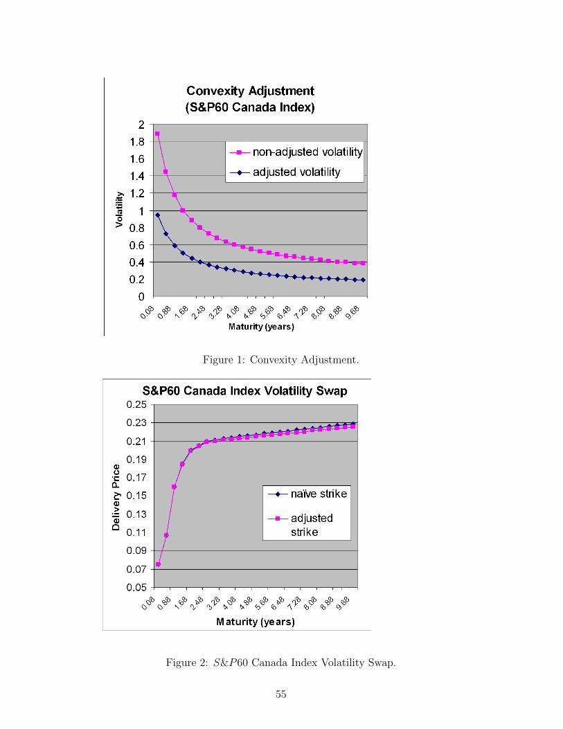
Figure 1: Convexity Adjustment.

Figure 2: S&P60 Canada Index Volatility Swap.

55

References

Avellaneda, M., Levy, A. and Paras, A. (1995): Pricing and hedg-ing derivative securities in markets with uncertain volatility, Appl. Math.Finance 2, 73-88.

Black, F. and Scholes, M. (1973): The pricing of options and corporateliabilities, J. Political Economy 81, 637-54.

Bollerslev, T. (1986): Generalized autoregressive conditional heteroscedas-ticity, J. Economics 31, 307-27.

Brockhaus, O. and Long, D. (2000): ”Volatility swaps made simple”,RISK, January, 92-96.

Buff, R. (2002): Uncertain volatility model. Theory and Applications.NY: Springer.

Carr, P. and Madan, D. (1998): Towards a Theory of Volatility Trading.In the book: Volatility, Risk book publications,http://www.math.nyu.edu/research/carrp/papers/.

Chesney, M. and Scott, L. (1989): Pricing European Currency Op-tions: A comparison of modifeied Black-Scholes model and a random variancemodel, J. Finan. Quantit. Anal. 24, No3, 267-284.

Cox, J., Ingersoll, J. and Ross, S. (1985): ”A theory of the termstructure of interest rates”, Econometrica 53, 385-407.

Demeterfi, K., Derman, E., Kamal, M. and Zou, J. (1999): A guideto volatility and variance swaps, The Journal of Derivatives, Summer, 9-32.

Duan, J. (1995): The GARCH option pricing model, Math. Finance 5,13-32.

Elliott, R. and Swishchuk, A. (2002): Studies of completeness ofBrownian and fractional (B, S,X)-securities markets. Working paper.

Frey, R. (1997): Derivative asset analysis in models with level-dependentand stochastic volatility, CWI Quarterly 10, 1-34.

Griego, R. and Swishchuk, A. (2000): Black-Scholes Formula for aMarket in a Markov Environment, Theory Probab. and Mathem. Statit. 62,9-18.

He, R. and Wang, Y. (2002): ”Price Pseudo-Variance, Pseudo Covari-ance, Pseudo-Volatility, and Pseudo-Correlation Swaps-In Analytical CloseForms”, RBC Financial Group, Query Note for 6th ISPW, PIMS, Vancouver,University of British Columbia, May 2002.

56

Heston, S. (1993): ”A closed-form solution for options with stochasticvolatility with applications to bond and currency options, Review of Finan-cial Studies, 6, 327-343

Hobson, D. and Rogers, L. (1998): Complete models with stochasticvolatility, Math. Finance 8, no.1, 27-48.

Hull, J. (2000): Options, futures and other derivatives, Prentice Hall, 4thedition.

Hull, J., and White, A. (1987): The pricing of options on assets withstochastic volatilities, J. Finance 42, 281-300.

Ikeda, N. and Watanabe, S. (1981): Stochastic Differential Equationsand Diffusion Processes, Kodansha Ltd., Tokyo.

Javaheri, A., Wilmott, P. and Haug, E. (2002): GARCH and volatil-ity swaps, Wilmott Technical Article, January, 17p.

Johnson, H. and Shanno, D. (1987): Option pricing when the varianceis changing, J. Finan. Quantit. Anal. 22,143-151.

Kazmerchuk, Y., Swishchuk, A., Wu, J. (2002): The pricing of op-tions for security markets with delayed response (submitted to MathematicalFinance journal).

Kazmerchuk, Y., Swishchuk, A. and Wu, J. (2002): A continuous-time GARCH model for stochastic volatility with delay, 18p. (Submitted toEuropean Journal of Applied Mathematics).

Merton, R. (1973): Theory of rational option pricing, Bell Journal ofEconomic Management Science 4, 141-183.

Øksendal, B. (1998): Stochastic Differential Equations: An Introductionwith Applications. NY: Springer.

”Price Pseudo-Variance, Pseudo-Covariance, Pseudo-Volatility, and Pseudo-Correlation Swaps-In Analytical Closed-Forms,” Proceedings of the SixthPIMS Industrial Problems Solving Workshop, PIMS IPSW 6, University ofBritish Columbia, Vancouver, Canada, May 27-31, 2002, pp. 45-55. Ed-itor: J. Macki, University of Alberta, June 2002. (So-joint report: Ray-mond Cheng, Stephen Lawi, Anatoliy Swishchuk, Andrei Bade-scu, Hammouda Ben Mekki, Asrat Fikre Gashaw, Yuanyuan Hua,Marat Molyboga, Tereza Neocleous, Yuri Petrachenko).

Scott, L. (1987): Option pricing when the variance changes randomly:theory, estimation and an application, J. Fin. Quant. Anal. 22, 419-438.

Stein, E. and Stein, J. (1991): Stock price distributions with stochasticvolatility: an analytic approach, Review Finan. Studies 4, 727-752.

57

Swishchuk, A. (1997): Hedging of options under mean-square criterionand with semi-Markov volatility, Ukrain. Math. J. 47, No7, 1119-1127.

Swishchuk, A. (2000): Random Evolutions and Their Applications. NewTrends, Kluwer Academic Publishers, Dordrecht, The Netherlands.

Swishchuk, A. and Kalemanova, A. (2000): Stochastic stability ofinterest rates with jumps. Theory probab. & Mathem statist., TBiMC Sci.Publ., v.61. (Preprint on-line: www.math.yorku.ca/˜aswishch/sample.html)

Swishchuk, A. (2004): Modeling and pricing of variance and volatilityswaps for financial markets with stochastic volatilities, Wilmott Magazine,Technical

Theoret, R., Zabre, L. and Rostan, P. (2002): Pricing volatilityswaps: empirical testing with Canadian data. Working paper, Centre deRecherche en Gestion, Document 17-2002, July 2002.

Wiggins, J. (1987): Option values under stochastic volatility: Theory andEmpirical Estimates, J. Finan. Econ. 19, 351-372.

Wilmott, P., Howison, S. and Dewynne, J. (1995): Option Pricing:Mathematical Models and Computations. Oxford: Oxford Financial Press.

58

Chapter 5: CTM and Delayed Heston Model:

Pricing and Hedging of Variance and Volatility

Swaps

’Better three hours too soon than a minute too late’,-William Shakespeare.

1 Introduction

In this chapter, we present a variance drift adjusted version of the Hestonmodel which leads to a significant improvement of the market volatility sur-face fitting (compared to Heston). The numerical example we performedwith recent market data shows a significant reduction of the average abso-lute calibration error 1 (calibration on 12 dates ranging from Sep. 19th toOct. 17th 2011 for the FOREX underlying EURUSD). Our model has twoadditional parameters compared to the Heston model, can be implementedvery easily and was initially introduced for volatility derivatives pricing pur-pose. The main idea behind our model is to take into account some pasthistory of the variance process in its (risk-neutral) diffusion. Using a changeof time method for continuous local martingales, we derive a closed formulafor the Brockhaus&Long approximation of the volatility swap price in thismodel. We also consider dynamic hedging of volatility swaps using a portfo-lio of variance swaps.

The volatility process is an important concept in financial modeling as itquantifies at each time t how likely the modeled asset log-return is to varysignificantly over some short immediate time period [t, t + ε]. This processcan be stochastic or deterministic, e.g. local volatility models in which the(deterministic) volatility depends on time and spot price level. In quanti-tative finance, we often consider the volatility process

√Vt (where Vt is the

variance process) to be stochastic as it allows to fit the observed vanilla op-tion market prices with an acceptable bias as well as to model the risk linkedwith the future evolution of the volatility smile (which deterministic modelcannot), namely the forward smile. Many derivatives are known to be verysensitive to the forward smile, one of the most popular example being thecliquet options (options on future asset performance, see Kruse and Nogel[18] for example).

Heston model (Heston [11]; Heston and Nandi [12]) is one of the most popularstochastic volatility models in the industry as semi-closed formulas for vanillaoption prices are available, few (five) parameters need to be calibrated, and

1The average absolute calibration error is defined to be the average of the absolutevalues of the differences between market and model implied Black & Scholes volatilities.

59

it accounts for the mean-reverting feature of the volatility.

One might be willing, in the variance diffusion, to take into account not onlyits current state but also its past history over some interval [t− τ, t], whereτ > 0 is a constant and is called the delay. Starting from the discrete-timeGARCH(1,1) model of Bollerslev [4]), a first attempt in this direction wasmade in Kazmerchuk et al. [16], where a non-Markov delayed continuous-time GARCH model was proposed (St being the asset price at time t, andγ, θ, α some positive constants). The dynamics considered had the form

dVtdt

= γθ2 +α

τln2

(StSt−τ

)− (α + γ)Vt. (1)

This model was inherited from its discrete-time analogue (where L is a pos-itive integer):

σ2n = γθ2 +

α

Lln2

(Sn−1Sn−1−L

)+ (1− α− γ)σ2

n−1. (2)

The parameter θ2 (resp. γ) can be interpreted as the value of the long-range variance (resp. variance mean-reversion speed) when the delay is equalto 0 (we will see that introducing a delay modifies the value of these twomodel features). α is a continuous-time equivalent of the variance ARCH(1,1)autoregressive coefficient. In fact, we can interpret the right-hand side of thediffusion equation (2) as the sum of two terms:

• the delay-free term γ(θ2 − Vt), which accounts for the mean-revertingfeature of the variance process

• α(

1τ

ln2(

StSt−τ

)− Vt

)which is a purely (noisy) delay term, i.e. one

that vanishes when τ → 0 and takes into account the past history of

the variance (via the term ln(

StSt−τ

)). The autoregressive coefficient α

can be seen as the amplitude of this purely delay term.

In Swishchuk [23] and Swishchuk and Li [21], the authors point out the im-portance of incorporating the real world P−drift dP(t, τ) :=

∫ tt−τ (µ−

12Vu)du

of ln(

StSt−τ

)in the model, where µ stands for the real world P−drift of the

stock price St, transforms the variance dynamics into:

dVtdt

= γθ2 +α

τ

[ln

(StSt−τ

)− dP(t, τ)

]2− (α + γ)Vt. (3)

The latter diffusion (3) was introduced in Swishchuk [23] and Kazmerchuk etal. [15], and the proposed model was proved to be complete and to accountfor the mean-reverting feature of the volatility process. This model is also

60

non Markov as the past history (Vu)u∈[t−τ,t] of the variance appears in its dif-

fusion equation via the term ln(

StSt−τ

), as shown in Swishchuk [23]. Following

this approach, a series of papers was published by one of the authors [23] fo-cusing on the pricing of variance swaps in this delayed framework: one-factorstochastic volatility with delay has been presented in Swishchuk [23]; multi-factor stochastic volatility with delay in Swishchuk [24]; one-factor stochasticvolatility with delay and jumps in Swishchuk and Li [21]; and finally localLevy-based stochastic volatility with delay in Swishchuk and Malenfant [26].

Other papers related to the concept of delay are also of interest. For exam-ple, Kind et al. [17] obtained a diffusion approximation result for processessatisfying some equations with past dependent coefficients, with applicationto option pricing. Arriojas et al. [1] derived a Black&Scholes formula forcall options assuming the stock price follows a Stochastic Delay Differen-tial Equation (SDDE). Mohammed and Bell have also published a series ofpapers in which they investigate various properties of SDDE (see e.g. [2], [3]).

Unfortunately, the model (3) doesn’t lead to (semi-)closed formulas for thevanilla options, making it difficult to use for practitioners willing to calibrateon vanilla market prices. Nevertheless, one can notice that the Heston modeland the delayed continuous-time GARCH model (3) are very similar in thesense that the expected values of the variances are the same - when we makethe delay tend to 0 in (3). As mentioned before, the Heston framework isvery convenient, and therefore it is naturally tempting to adjust the Hestondynamics in order to incorporate the delay introduced in (3). In this way, weconsidered in a first approach adjusting the Heston drift by a deterministicfunction of time so that the expected value of the variance under the delayedHeston model is equal to the one under the delayed GARCH model (3). Inaddition to making our delayed Heston framework coherent with (3), thisconstruction makes the variance process diffusion dependent not on its pasthistory (Vu)u∈[t−τ,t], but on the past history of its risk-neutral expectation

(EQ0 (Vu))u∈[t−τ,t], preserving the Markov feature of the Heston model (where

we denote EQt (·) := EQ(·|Ft) for some filtration (Ft)t≥0). The purpose of

sections 2 and 3 is to present the Delayed Heston model as well as some cali-bration results on call option prices, with a comparison to the Heston model.In sections 4 and 5, we will consider the pricing and hedging of volatility andvariance swaps in this model.

Volatility and variance swaps are contracts whose payoff depend (respectivelyconvexly and linearly) on the realized variance of the underlying asset oversome specified time interval. They provide pure exposure to volatility, andtherefore make it a tradable market instrument. Variance Swaps are evenconsidered by some practitioners to be vanilla derivatives. The most com-monly traded variance swaps are discretely sampled and have a payoff P V

n (T )

61

at maturity T of the form:

P Vn (T ) = N

[252

n

n∑i=0

ln2

(Si+1

Si

)−Kvar

],

where Si is the asset spot price on fixing time ti ∈ [0, T ] (usually there isone fixing time each day, but there could be more, or less), N the notionalamount of the contract (in currency per unit of variance) and Kvar the strikespecified in the contract. The corresponding volatility swap payoff P v

n (T ) isgiven by:

P vn (T ) = N

√√√√252

n

n∑i=0

ln2

(Si+1

Si

)−Kvol

.One can also consider continuously sampled volatility and variance swaps (onwhich we will focus in this article), which payoffs are respectively defined asthe limit when n→ +∞ of their discretely sampled versions. Formally, if wedenote (Vt)t≥0 the stochastic volatility process of our asset, adapted to somebrownian filtration (Ft)t≥0, then the continuously-sampled realized varianceVR from initiation date of the contract t = 0 to maturity date t = T is givenby VR = 1

T

∫ T0Vsds. The fair variance strike Kvar is calculated such that the

initial value of the contract is 0, and therefore is given by:

EQ0

[e−rT (VR −Kvar)

]= 0⇒ Kvar = EQ

0 (VR).

In the same way, the fair volatility strike Kvol is given by:

EQ0

[e−rT (

√VR −Kvol)

]= 0⇒ Kvol = EQ

0 (√VR).

The volatility swap fair strike might be difficult to compute explicitly as wehave to compute the expectation of a square-root. In Brockhaus and Long [7],the following approximation - based on a Taylor expansion - was proposedto compute the expected value of the square-root of an almost surely nonnegative random variable Z:

E(√Z) ≈

√E(Z)− V ar(Z)

8E(Z)32

. (4)

We will refer to this approximation in our paper as the Brockhaus&Longapproximation.

There exists a vast literature on volatility and variance swaps. We provide inthe following lines a selection of papers covering important topics. Carr andLee [8] provides an overview of the current market of volatility derivatives.They survey the early literature on the subject. They also provide relativelysimple proofs of some fundamental results related to variance swaps and

62

volatility swaps. Pricing of variance swaps for one-factor stochastic volatilityis presented in Swishchuk [22]. Variance and volatility swaps in energy mar-kets are considered in Swishchuk [25]. Broadie and Jain [6] covers pricingand dynamic hedging of volatility derivatives in the Heston model. More-over, various papers deal with the VIX Index - the Chicago Board OptionsExchange Market Volatility Index - which is a popular measure of the onemonth implied volatility on the S&P 500 index (see e.g. Zhang and Zhu [28],Hao and Zhang [10] or Filipovic [9]).

The paper is organized as follows: in section 2, we present the DelayedHeston model; in section 3, we present calibration results (for underlyingEURUSD on 12 dates ranging from Sep. 19th to Oct. 17th 2011 2011) aswell as a comparison with the Heston model. In section 4, we compute theprice process Xt(T ) := EQ

t (VR) of the floating leg of the variance swap ofmaturity T , as well as the Brockhaus&Long approximation of the price pro-cess Yt(T ) := EQ

t (√VR) of the floating leg of the volatility swap of maturity

T . This leads in particular to closed formulas for the fair volatility and vari-ance strikes. In section 5, we consider - in this model - dynamic hedging ofvolatility swaps using variance swaps.

2 Presentation of the Delayed Heston model

Throughout this paper, we will assume constant risk-free rate r, dividendyield q and finite time-horizon T . We fix (Ω,F ,P) a probability space andwe consider a stock whose price process is denoted by (St)t≥0. We let Q be arisk-neutral measure and we let (ZQ

t )t≥0 and (WQt )t≥0 be two correlated stan-

dard brownian motions on (Ω,F ,Q). We let the natural filtration associatedto these brownian motions Ft := σ(ZQ

t ,WQt ) and we denote EQ

t (·) := EQ(·|Ft)and V arQt (·) := V arQ(·|Ft).

We assume the following risk-neutral Q− stock price dynamics :

dSt = (r − q)Stdt+ St√VtdZ

Qt . (5)

The well-known Heston model has the following Q−dynamics for the varianceVt:

dVt = γ(θ2 − Vt)dt+ δ√VtdW

Qt , (6)

where θ2 is the long-range variance, γ the variance mean-reversion speed,δ the volatility of the variance and ρ the brownian correlation coefficient(⟨WQ, ZQ

⟩t

= ρt). We also assume S0 = s0 a.e. and V0 = v0 a.e., for somepositive constants v0, s0.

63

As explained in the introduction, the following delayed continuous-time GARCHdynamics have been introduced for the variance in Swishchuk [23]:

dVtdt

= γθ2 +α

τ

[∫ t

t−τ

√VsdZ

Qs − (µ− r)τ

]2− (α + γ)Vt, (7)

where µ stands for the real world P−drift of the stock price St. We noticethat θ2 (resp. γ) has been defined in introduction for the delayed continuous-time GARCH model as the value of the long-range variance (resp. variancemean-reversion speed) when τ = 0, therefore it has the same meaning as theHeston long-range variance (resp. variance mean-reversion speed). That iswhy we use the same notations in both models.

We can see that the two models are very similar. Indeed, they both givethe same expected value for Vt as the delay goes to 0 in (7), namely θ2 +(V0− θ2)e−γt. The idea here is to adjust the Heston dynamics (6) in order toaccount for the delay introduced in (7). Our approach is to adjust the driftby a deterministic function of time so that the expected value of Vt underthe adjusted Heston model is the same as under (7). This approach can beseen as a correction by a pure delay term of amplitude α of the Heston driftby a deterministic function in order to account for the delay.

Namely, we assume the adjusted Heston dynamics:

dVt =[γ(θ2 − Vt) + ετ (t)

]dt+ δ

√VtdW

Qt , (8)

ετ (t) := ατ(µ− r)2 +α

τ

∫ t

t−τvsds− αvt, (9)

with vt := EQ0 (Vt). It was shown in Swishchuk [23] that vt solves the following

equation:

dvtdt

= γθ2 + ατ(µ− r)2 +α

τ

∫ t

t−τvsds− (α + γ)vt, (10)

and that we have the following expression for vt:

vt = θ2τ + (V0 − θ2τ )e−γτ t, (11)

with:

θ2τ := θ2 +ατ(µ− r)2

γ. (12)

By (11) and (15) (see below), we have limt→∞ vt = θ2τ and therefore theparameter θ2τ can be interpreted as the adjusted value of the limit towards vttends to as t→∞, that has been (positively) shifted from its original valueθ2 because of the introduction of delay. We have θ2τ → θ2 when τ → 0, whichis coherent. We will see below that we can interpret the parameter γτ > 0

64

as the adjusted mean-reversion speed. This parameter is given in Swishchuk[23] by a (nonzero) solution to the following equation:

γτ = α + γ +α

γττ(1− eγτ τ ). (13)

By (9), (11) and (13) we get an explicit expression for the drift adjustment:

ετ (t) = ατ(µ− r)2 + (V0 − θ2τ )(γ − γτ )e−γτ t. (14)

The following simple property gives us some information about the correc-tion term ετ (t) and the parameter γτ , that will be useful for interpretationpurpose and in the derivation of the semi-closed formulas for call options inAppendix A. Indeed, given (15) and (11), the parameter γτ can be inter-preted as the adjusted variance mean-reversion speed because it quantifiesthe speed at which vt tends to θ2τ as t→∞, and we have by using a Taylorexpansion in (13) that γτ → γ when τ → 0, which is coherent.

Property 1: γτ is the unique solution to (13) and:

0 < γτ < γ, limτ→0

supt∈R+

|ετ (t)| = 0. (15)

Proof : Let’s show γτ ≥ 0. If γτ < 0 then by (13) we have α+γ+ αγτ τ

(1−eγτ τ ) < 0,

i.e. 1 − eγτ τ + γττ > − γαγττ . But τ > 0 so ∃x0 > 0 s.t. 1 − e−x0 − x0 > γ

αx0.

A simple study shows that is impossible whenever γα ≥ 0, which is what we have

by assumption. Therefore γτ ≥ 0, and in fact γτ > 0 since it is a nonzero solu-

tion of (13). If γ ≤ γτ then by (13) γττ + 1 − eγτ τ ≥ 0. But γττ > 0 therefore

∃x0 > 0 s.t. x0 + 1 − ex0 ≥ 0. A simple study shows that is impossible. The

uniqueness comes from a similar simple study. Now, because γτ > 0, we have

supt∈R+

|ετ (t)| ≤ ατ(µ− r)2 + |(V0− θ2τ )(γ−γτ )| and (V0− θ2τ )(γ−γτ ) = (1) by (13).

So limτ→0

ατ(µ− r)2 + |(V0 − θ2τ )(γ − γτ )| = 0.

Using (14) and (12), we can rewrite (8) as a time-dependent Heston modelwith time-dependent long-range variance θ2t :

dVt = γ(θ2t − Vt)dt+ δ√VtdW

Qt , (16)

θ2t := θ2τ + (V0 − θ2τ )(γ − γτ )

γe−γτ t. (17)

The parameter θ2τ is - as we mentioned above - the adjusted value of thelimit towards which vt tends to as t → ∞. For this reason, it is coherentthat it is also the limiting value of the time-dependent long-range varianceθ2t as t→∞ (by (17) and (15)).

65

3 Calibration on call option prices and com-

parison to the Heston model

Following Kahl and Jackel [13] and Mikhailov and Noegel [20], it is possibleto get semi-closed formulas for call options in our delayed Heston model.Indeed, our model is a time-dependent Heston model with time-dependentlong-range variance θ2t . We refer to Appendix A for the procedure to derivesuch semi-closed formulas.

We perform our calibration on September 30th 2011 for underlying EURUSDon the whole volatility surface (maturities from 1M to 10Y, strikes ATM, 25DCall/Put, 10D Call/Put). The implied volatility surface, the Zero Couponcurves EUR Vs. Euribor 6M and USD Vs. Libor 3M and the spot price aretaken from Bloomberg (mid prices). The drift µ = 0.0188 is estimated from7.5Y of daily close prices (source: www.forexrate.co.uk).

The calibration procedure is a least-squares minimization procedure that weperform via MATLAB (function lsqnonlin that uses a trust-region-reflectivealgorithm). The Heston integral (83) is computed via the MATLAB func-tion quadl that uses a recursive adaptive Lobatto quadrature. The integral∫ t0e−γτ sD(s, u)ds in (81) is computed via a composite Simpson’s rule with

100 points.

The calibrated parameters for delayed Heston are:

(V0, γ, θ2, δ, ρ, α, τ) = (0.0343, 3.9037, 10−8, 0.808,−0.5057, 71.35, 0.7821),

and for Heston, they are:

(V0, γ, θ2, δ, ρ) = (0.0328, 0.5829, 0.0256, 0.3672,−0.4824).

We notice that we cannot compare straightforwardly the parameters θ2 ofboth models. Indeed, as mentioned above, the Delayed Heston model has atime-dependent long range variance θ2t which has been shifted away from itsoriginal value θ2 because of the introduction of the delay τ . When τ = 0,θ2t = θ2 but when τ > 0, θ2t and θ2 differ. Therefore, to be coherent, oneshould compare the Heston long range-variance θ2 = 0.0256 with the DelayedHeston time-dependent long-range variance θ2t . Below we give the value ofθ2t for different maturities t:

Maturity θ2t1M 0.03252M 0.03223M 0.03196M 0.0311Y 0.02942Y 0.03645Y 0.018410Y 0.0102

66

Table 1: Parameter θ2t for different maturities t.

We remark that the short and medium term values (less than 2Y) of θ2t aresimilar to the value of θ2 in the Heston model, but that for long maturities,the value of θ2t decreases significantly. Allowing this time-dependence of thethe long-range variance could be an explanation why the Delayed Hestonmodel outperforms the Heston model especially for long maturities (see thediscussion below). Similarly, the Heston mean-reversion speed γ = 0.58 hasto be compared with the Delayed Heston adjusted mean-reversion speed γτ ,which is given by (13) and is approximately equal to 0.12 on our calibrationdate. Focusing on the delay parameters α and τ , they were expected to besignificantly non zero because as we will see below, the Delayed Heston modelsignificantly outperforms the Heston model in terms of calibration error (andstandard deviation of the calibration errors): if α and τ were close to 0, thecalibration errors would have been approximately the same for both models,because again, the Delayed Heston model reduces to the Heston model whenthe delay term vanishes, i.e. when τ = 0 or α = 0.

The calibration errors for all call options (expressed as the absolute value ofthe difference between market and model implied Black & Scholes volatili-ties, in bp) for the Heston model and our Delayed Heston model are givenbelow. The results show a 44% reduction of the average absolute calibrationerror (46bp for delayed Heston, 81bp for Heston). It is to be noted that wedidn’t use any weight matrix in our calibration procedure, i.e. the calibrationaims at minimizing the sum of the (squares of the) errors of each call option,equally weighted. In practice, one might be willing to give more importanceto ATM options for instance, or options of a certain range of maturities. Theoptimization algorithm aims at minimizing the sum of the squares of the er-rors: in other words, it aims at minimizing the average absolute calibrationerror. For this reason, it might be the case that for some specific option(e.g. ATM 6M, see table below), the Heston model has a lower model errorthan the Delayed Heston model. But the total calibration error for the De-layed Heston model is always expected to be lower than for the Heston model.

On our calibration date, the Delayed Heston model seems to outperform theHeston model specifically for long maturities (≥ 3Y): if we consider onlythese options, the average absolute error is of 79bp for the Heston modeland 33bp for the Delayed Heston model, which represents a 58% reductionof the calibration error. We can also note that for ATM options only, theimprovement is significant too (43bp Vs. 92bp, i.e. an error reduction of54%). For medium maturity options (6M to 2Y), the Delayed Heston modelstill outperforms the Heston model but less significantly (53bp Vs. 75bp, i.e.an error reduction of 30%), and we have the same observation for very outof the money options (10 Delta Call and Put, 51bp Vs. 79bp, i.e. an error

67

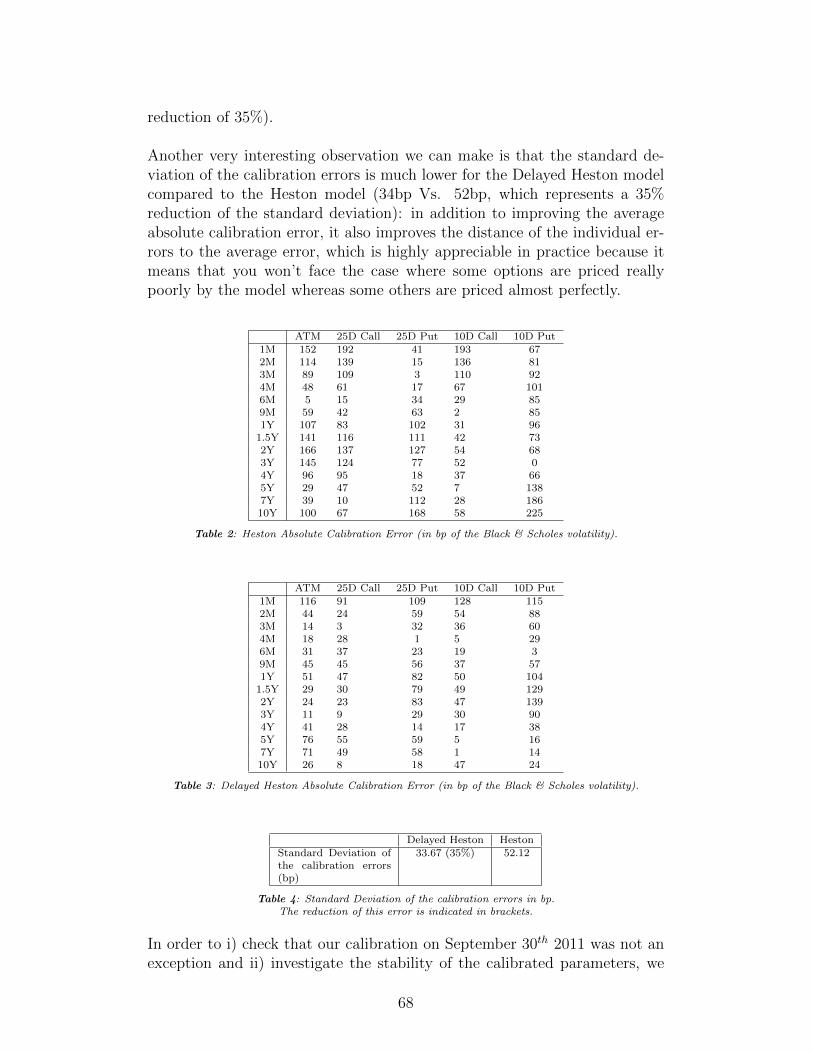
reduction of 35%).

Another very interesting observation we can make is that the standard de-viation of the calibration errors is much lower for the Delayed Heston modelcompared to the Heston model (34bp Vs. 52bp, which represents a 35%reduction of the standard deviation): in addition to improving the averageabsolute calibration error, it also improves the distance of the individual er-rors to the average error, which is highly appreciable in practice because itmeans that you won’t face the case where some options are priced reallypoorly by the model whereas some others are priced almost perfectly.

ATM 25D Call 25D Put 10D Call 10D Put1M 152 192 41 193 672M 114 139 15 136 813M 89 109 3 110 924M 48 61 17 67 1016M 5 15 34 29 859M 59 42 63 2 851Y 107 83 102 31 961.5Y 141 116 111 42 732Y 166 137 127 54 683Y 145 124 77 52 04Y 96 95 18 37 665Y 29 47 52 7 1387Y 39 10 112 28 18610Y 100 67 168 58 225

Table 2: Heston Absolute Calibration Error (in bp of the Black & Scholes volatility).

ATM 25D Call 25D Put 10D Call 10D Put1M 116 91 109 128 1152M 44 24 59 54 883M 14 3 32 36 604M 18 28 1 5 296M 31 37 23 19 39M 45 45 56 37 571Y 51 47 82 50 1041.5Y 29 30 79 49 1292Y 24 23 83 47 1393Y 11 9 29 30 904Y 41 28 14 17 385Y 76 55 59 5 167Y 71 49 58 1 1410Y 26 8 18 47 24

Table 3: Delayed Heston Absolute Calibration Error (in bp of the Black & Scholes volatility).

Delayed Heston HestonStandard Deviation ofthe calibration errors(bp)

33.67 (35%) 52.12

Table 4: Standard Deviation of the calibration errors in bp.The reduction of this error is indicated in brackets.

In order to i) check that our calibration on September 30th 2011 was not anexception and ii) investigate the stability of the calibrated parameters, we

68

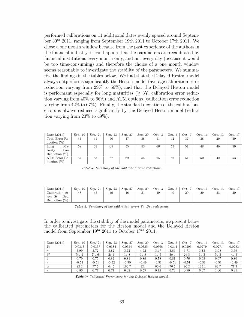
performed calibrations on 11 additional dates evenly spaced around Septem-ber 30th 2011, ranging from September 19th 2011 to October 17th 2011. Wechose a one month window because from the past experience of the authors inthe financial industry, it can happen that the parameters are recalibrated byfinancial institutions every month only, and not every day (because it wouldbe too time-consuming) and therefore the choice of a one month windowseems reasonable to investigate the stability of the parameters. We summa-rize the findings in the tables below. We find that the Delayed Heston modelalways outperforms significantly the Heston model (average calibration errorreduction varying from 29% to 56%), and that the Delayed Heston modelis performant especially for long maturities (≥ 3Y, calibration error reduc-tion varying from 40% to 66%) and ATM options (calibration error reductionvarying from 42% to 67%). Finally, the standard deviation of the calibrationserrors is always reduced significantly by the Delayed Heston model (reduc-tion varying from 23% to 49%).

Date (2011) Sep. 19 Sep. 21 Sep. 23 Sep. 27 Sep. 29 Oct. 3 Oct. 5 Oct. 7 Oct. 11 Oct. 13 Oct. 17Total Error Re-duction (%)

44 45 56 47 38 51 42 37 38 29 39

Long Ma-turity ErrorReduction (%)

58 63 65 55 53 66 55 51 48 40 59

ATM Error Re-duction (%)

57 55 67 62 55 65 56 51 50 42 53

Table 5: Summary of the calibration error reductions.

Date (2011) Sep. 19 Sep. 21 Sep. 23 Sep. 27 Sep. 29 Oct. 3 Oct. 5 Oct. 7 Oct. 11 Oct. 13 Oct. 17Calibration er-rors St. Dev.Reduction (%)

43 45 49 46 31 49 40 29 29 23 29

Table 6: Summary of the calibration errors St. Dev reductions.

In order to investigate the stability of the model parameters, we present belowthe calibrated parameters for the Heston model and the Delayed Hestonmodel from September 19th 2011 to October 17th 2011.

Date (2011) Sep. 19 Sep. 21 Sep. 23 Sep. 27 Sep. 29 Oct. 3 Oct. 5 Oct. 7 Oct. 11 Oct. 13 Oct. 17V0 0.0313 0.0337 0.0384 0.0354 0.0335 0.0368 0.0344 0.0295 0.0279 0.0271 0.0283γ 3.99 3.72 3.82 3.72 4.52 3.47 3.86 3.71 3.13 3.08 3.39θ2 5 e-4 7 e-6 2e-4 1e-8 1e-8 1e-5 3e-4 2e-3 1e-3 5e-3 4e-3δ 0.79 0.75 0.82 0.81 0.89 0.78 0.81 0.76 0.68 0.67 0.80ρ -0.51 -0.51 -0.52 -0.50 -0.49 -0.51 -0.51 -0.51 -0.51 -0.51 -0.49α 82.2 77.5 64.5 166.7 124 66.6 76.5 90.2 125.1 83.7 77.3τ 0.86 0.77 0.71 0.32 0.59 0.72 0.78 0.90 0.67 1.00 0.81

Table 7: Calibrated Parameters for the Delayed Heston model.

69

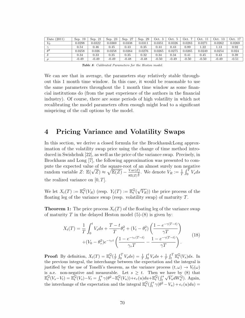
Date (2011) Sep. 19 Sep. 21 Sep. 23 Sep. 27 Sep. 29 Oct. 3 Oct. 5 Oct. 7 Oct. 11 Oct. 13 Oct. 17V0 0.0298 0.0322 0.0369 0.0338 0.0311 0.0351 0.0326 0.0283 0.0271 0.0262 0.0269γ 0.54 0.46 0.45 0.43 0.35 0.44 0.43 0.89 1.22 1.13 0.92θ2 0.0258 0.026 0.0258 0.0264 0.0276 0.0265 0.0275 0.0265 0.0249 0.0254 0.024δ 0.34 0.33 0.35 0.35 0.32 0.34 0.34 0.41 0.45 0.43 0.39ρ -0.49 -0.49 -0.49 -0.48 -0.48 -0.50 -0.49 -0.50 -0.50 -0.49 -0.51

Table 8: Calibrated Parameters for the Heston model.

We can see that in average, the parameters stay relatively stable through-out this 1 month time window. In this case, it would be reasonable to usethe same parameters throughout the 1 month time window as some finan-cial institutions do (from the past experience of the authors in the financialindustry). Of course, there are some periods of high volatility in which notrecalibrating the model parameters often enough might lead to a significantmispricing of the call options by the model.

4 Pricing Variance and Volatility Swaps

In this section, we derive a closed formula for the Brockhaus&Long approx-imation of the volatility swap price using the change of time method intro-duced in Swishchuk [22], as well as the price of the variance swap. Precisely, inBrockhaus and Long [7], the following approximation was presented to com-pute the expected value of the square-root of an almost surely non negativerandom variable Z: E(

√Z) ≈

√E(Z)− V ar(Z)

8E(Z)32

. We denote VR := 1T

∫ T0Vsds

the realized variance on [0, T ].

We let Xt(T ) := EQt (VR) (resp. Yt(T ) := EQ

t (√VR)) the price process of the

floating leg of the variance swap (resp. volatility swap) of maturity T .

Theorem 1: The price process Xt(T ) of the floating leg of the variance swapof maturity T in the delayed Heston model (5)-(8) is given by:

Xt(T ) =1

T

∫ t

0

Vsds+T − tT

θ2τ + (Vt − θ2τ )(

1− e−γ(T−t)

γT

)+(V0 − θ2τ )e−γτ t

(1− e−γτ (T−t)

γτT− 1− e−γ(T−t)

γT

).

(18)

Proof: By definition, Xt(T ) = EQt ( 1

T

∫ T0 Vsds) = 1

T

∫ t0 Vsds + 1

T

∫ Tt EQ

t (Vs)ds. Inthe previous integral, the interchange between the expectation and the integral isjustified by the use of Tonelli’s theorem, as the variance process (t, ω) → Vt(ω)is a.e. non-negative and measurable. Let s ≥ t. Then we have by (8) thatEQt (Vs−Vt) = EQ

t (Vs)−Vt =∫ st γ(θ2−EQ

t (Vu))+ετ (u)du+EQt (∫ st

√VudW

Qu ). Again,

the interchange of the expectation and the integral EQt (∫ st γ(θ2−Vu) + ετ (u)du) =

70

∫ st γ(θ2 − EQ

t (Vu)) + ετ (u)du is obtained the following way:

EQt (

∫ s

tγ(θ2 − Vu) + ετ (u)du) =

∫ s

tγθ2 + ετ (u)du− γEQ

t (

∫ s

tVudu). (19)

Then again, by Tonelli’s theorem we get EQt (∫ st Vudu) =

∫ st EQ

t (Vu)du, which jus-

tifies the interchange.

Now, (√Vt)t≥0 is an adapted process (to our filtration (Ft)t≥0) s.t. EQ(

∫ T0 Vudu) =∫ T

0 EQ(Vu)du < +∞ (by Tonelli’s theorem), therefore∫ t0

√VudW

Qu is a martingale

and we have EQt (∫ st

√VudW

Qu ) = 0. Therefore ∀s ≥ t ≥ 0, the function s→ EQ

t (Vs)

is a solution of y′s = γ(θ2− ys) + ετ (s) with initial condition yt = Vt. This gives us

EQt (Vs) = θ2τ + (Vt − θ2τ )e−γ(s−t) + (V0 − θ2τ )e−γτ t(e−γτ (s−t) − e−γ(s−t)). Integrating

the latter in the variable s via∫ Tt EQ

t (Vs)ds completes the proof.

Corollary 1: The price Kvar of the variance swap of maturity T at initiationof the contract t = 0 in the delayed Heston model (5)-(8) is given by:

Kvar = θ2τ + (V0 − θ2τ )1− e−γτT

γτT. (20)

Proof: By definition, Kvar = X0(T ).

Now, let:

xt := −(V0 − θ2τ )e(γ−γτ )t + eγt(Vt − θ2τ ). (21)

Then by Ito’s Lemma we get:

dxt = δeγt√

(xt + (V0 − θ2τ )e(γ−γτ )t)e−γt + θ2τdWQt . (22)

Which is of the form dxt = f(t, xt)dWQt with:

f(t, x) := δeγt√

(x+ (V0 − θ2τ )e(γ−γτ )t)e−γt + θ2τ . (23)

Indeed, since xt = g(t, Vt) with g(t, x) := −(V0− θ2τ )e(γ−γτ )t + eγt(x− θ2τ ), themultidimensional version of Ito’s lemma reads:

dxt = dg(t, Vt) = gt(t, Vt)dt+ gx(t, Vt)dVt +1

2gxx(t, Vt)d 〈V, V 〉t , (24)

71

where 〈V, V 〉t is the quadratic variation of the process (Vt)t≥0 (see e.g. [14],theorem 3.6. of section 3.3). Since gxx(t, x) = 0, gt(t, Vt) = −(γ − γτ )(V0 −θ2τ )e

(γ−γτ )t+γeγt(Vt−θ2τ ) and gx(t, Vt) = eγt, we get, using (8), (12) and (14):

dxt =gt(t, Vt)dt+ gx(t, Vt)dVt (25)

=− (γ − γτ )(V0 − θ2τ )e(γ−γτ )tdt+ γeγt(Vt − θ2τ )dt+ eγtdVt (26)

=− eγt(ετ (t)− γ(θ2τ − θ2))dt+ γeγt(Vt − θ2τ )dt (27)

+ eγt[γ(θ2 − Vt) + ετ (t)

]dt+ eγtδ

√VtdW

Qt (28)

=eγtδ√VtdW

Qt . (29)

The fact that Vt = (xt + (V0 − θ2τ )e(γ−γτ )t)e−γt + θ2τ by definition of xt (21)completes the proof.

Because dxt = f(t, xt)dWQt , the process (xt)t≥0 is a continuous local martin-

gale, and even a true martingale since EQ(∫ T0f 2(s, xs)ds) =

∫ T0EQ(f 2(s, xs))ds <

∞ (again, the interchange between expectation and integral follows fromTonelli’s theorem). We can use the change of time method introducedin Swishchuk [22] and we get xt = Wφt , where Wt is a Fφ−1

t− adapted

Q−Brownian motion, which is based on the fact that every continuous localmartingale can be represented as a time-changed brownian motion. The pro-cess (φt)t≥0 is a.e. increasing, non negative, Ft− adapted and is called thechange of time process. This process is also equal to the quadratic variation〈x〉t of the (square-integrable) continuous martingale xt (see [14], section 3.2,Proposition 2.10.).

Expressions of φt, φ−1t and Wt are given by:

φt = 〈x〉t =

∫ t

0

f 2 (s, xs) ds, (30)

Wt =

∫ φ−1t

0

f(s, xs)dWQs , (31)

φ−1t =

∫ t

0

1

f 2(φ−1s , xφ−1

s

)ds. (32)

To see that φ−1t has the following form, observe that:

φ−1φt =

∫ φt

0

1

f 2(φ−1s , xφ−1

s

)ds. (33)

Now make the change of variable s = φu, so that ds = dφu = f 2 (u, xu) du.We get:

φ−1φt =

∫ t

0

f 2 (u, xu)

f 2(φ−1φu , xφ−1

φu

)du =

∫ t

0

f 2 (u, xu)

f 2 (u, xu)du = t. (34)

72

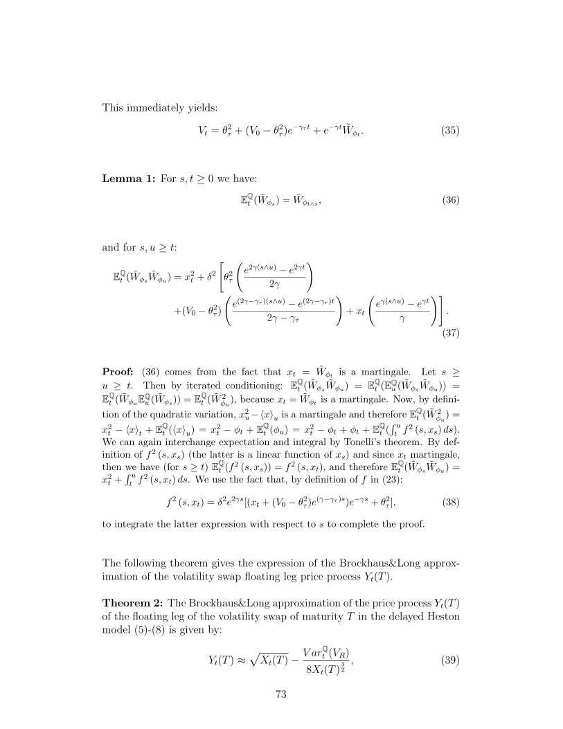
This immediately yields:

Vt = θ2τ + (V0 − θ2τ )e−γτ t + e−γtWφt . (35)

Lemma 1: For s, t ≥ 0 we have:

EQt (Wφs) = Wφt∧s , (36)

and for s, u ≥ t:

EQt (WφsWφu) = x2t + δ2

[θ2τ

(e2γ(s∧u) − e2γt

2γ

)

+(V0 − θ2τ )

(e(2γ−γτ )(s∧u) − e(2γ−γτ )t

2γ − γτ

)+ xt

(eγ(s∧u) − eγt

γ

)].

(37)

Proof: (36) comes from the fact that xt = Wφt is a martingale. Let s ≥u ≥ t. Then by iterated conditioning: EQ

t (WφsWφu) = EQt (EQ

u (WφsWφu)) =

EQt (WφuEQ

u (Wφs)) = EQt (W 2

φu), because xt = Wφt is a martingale. Now, by defini-

tion of the quadratic variation, x2u−〈x〉u is a martingale and therefore EQt (W 2

φu) =

x2t − 〈x〉t + EQt (〈x〉u) = x2t − φt + EQ

t (φu) = x2t − φt + φt + EQt (∫ ut f

2 (s, xs) ds).We can again interchange expectation and integral by Tonelli’s theorem. By def-inition of f2 (s, xs) (the latter is a linear function of xs) and since xt martingale,then we have (for s ≥ t) EQ

t (f2 (s, xs)) = f2 (s, xt), and therefore EQt (WφsWφu) =

x2t +∫ ut f

2 (s, xt) ds. We use the fact that, by definition of f in (23):

f2 (s, xt) = δ2e2γs[(xt + (V0 − θ2τ )e(γ−γτ )s)e−γs + θ2τ ], (38)

to integrate the latter expression with respect to s to complete the proof.

The following theorem gives the expression of the Brockhaus&Long approx-imation of the volatility swap floating leg price process Yt(T ).

Theorem 2: The Brockhaus&Long approximation of the price process Yt(T )of the floating leg of the volatility swap of maturity T in the delayed Hestonmodel (5)-(8) is given by:

Yt(T ) ≈√Xt(T )− V arQt (VR)

8Xt(T )32

, (39)

73

where Xt(T ) is given by equation (18) of Theorem 1 and:

V arQt (VR) =xtδ

2

γ3T 2

[e−γt

(1− e−2γ(T−t)

)− 2(T − t)γe−γT

]+

δ2

2γ3T 2

[2θ2τγ(T − t)+ 2(V0 − θ2τ )

γ

γτe−γτ t + 4θ2τe

−γ(T−t) − θ2τe−2γ(T−t) − 3θ2τ

]− δ2(V0 − θ2τ )

γ2T 2(γ2τ + 2γ2 − 3γγτ )[ 2(γτ − 2γ)e−γ(T−t)−γτ t

+(γ − γτ )e−2γ(T−t)−γτ t + 2γ2

γτe−γτT

].

(40)

Proof: The (conditioned) Brockhaus&Long approximation gives us:

Yt(T ) = EQt (√VR) ≈

√EQt (VR)− V arQt (VR)

8EQt (VR)

32

=√Xt(T )− V arQt (VR)

8Xt(T )32

.

Furthermore:

V arQt (VR) = EQt ((VR − EQ

t (VR))2)

=1

T 2EQt

((∫ T

0(Vs − EQ

t (Vs))ds

)2).

(41)

From (35) we have Vt = θ2τ + (V0− θ2τ )e−γτ t + e−γtWφt , and since Wφt is a martin-

gale, Vs − EQt (Vs) = 0 if s ≤ t, and Vs − EQ

t (Vs) = e−γs(Wφs − xt) if s > t.

Therefore:

V arQt (VR) =1

T 2EQt

((∫ T

te−γs(Wφs − xt)ds

)2)

=1

T 2x2t

(∫ T

te−γsds

)2

+1

T 2EQt

((∫ T

te−γsWφsds

)2)

− 2

T 2xt

(∫ T

te−γsEQ

t (Wφs)ds

)(∫ T

te−γsds

).

(42)

The interchange of expectation and integral in the last equation is justified thefollowing way: by definition of Wφs = xs in (21), we get:

EQt (

∫ T

te−γsWφsds) = EQ

t (

∫ T

t−(V0 − θ2τ )e−γτ s + Vs − θ2τds) (43)

=

∫ T

t−(V0 − θ2τ )e−γτ s − θ2τds+ EQ

t (

∫ T

tVsds). (44)

We can interchange expectation and integral in the latter expression by Tonelli’s

74

theorem, which gives:

EQt (

∫ T

te−γsWφsds) =

∫ T

t−(V0 − θ2τ )e−γτ s − θ2τds+

∫ T

tEQt (Vs)ds (45)

=

∫ T

te−γsEQ

t (Wφs)ds. (46)

Now we continue our computation to get:

V arQt (VR) = − 1

T 2x2t

(∫ T

te−γsds

)2

+1

T 2EQt

((∫ T

te−γsWφsds

)2)

=1

T 2

∫ T

t

∫ T

te−γ(s+u)EQ

t (WφsWφu)dsdu− 1

T 2x2t e−2γt

(1− e−γ(T−t)

γ

)2

.

(47)

The interchange expectation-integral:

EQt (

∫ T

t

∫ T

te−γ(s+u)WφsWφudsdu) =

∫ T

t

∫ T

te−γ(s+u)EQ

t (WφsWφu)dsdu (48)

is justified the same way as above, using the definition of Wφt = xt in (21) togetherwith Tonelli’s theorem. Finally, we use equation (37) of Lemma 1 and integratethe expression with respect to s and u to complete the proof.

Corollary 2: The Brockhaus&Long approximation of the volatility swapprice Kvol of maturity T at initiation of the contract t = 0 in the delayedHeston model (5)-(8) is given by:

Kvol ≈√Kvar −

V arQ0 (VR)

8K32var

, (49)

where Kvar is given by formula (20) of Corollary 1 and:

V arQ0 (VR) =δ2e−2γT

2T 2γ3

[θ2τ(2γTe2γT + 4eγT − 3e2γT − 1

)+

γ

2γ − γτ(V0 − θ2τ )(

2e2γT(

2γ

γτ− 1

)− 4γeγT

(e(γ−γτ )T − 1

γ − γτ

)+ 4eγT

(1− γ

γτe(γ−γτ )T

)− 2

)].

(50)

We notice that letting τ → 0 (and therefore γτ → γ) we get the formula ofSwishchuk [22].

Proof: We have by definition Kvol = Y0(T ), therefore the result is obtained fromequation (40) of Theorem 2.

75

5 Volatility Swap Hedging

In this section, we consider dynamic hedging of volatility swaps using varianceswaps, as the latter are a fairly liquid, easy to trade derivatives. In the spiritof Broadie and Jain [6], we consider a portfolio containing at time t oneunit of volatility swap and βt units of variance swaps, both of maturity T .Therefore the value Πt of the portfolio at time t is:

Πt = e−r(T−t) [Yt(T )−Kvol + βt(Xt(T )−Kvar)] . (51)

The portfolio is self-financing, therefore:

dΠt = rΠtdt+ e−r(T−t) [dYt(T ) + βtdXt(T )] . (52)

The price processes Xt(T ) and Yt(T ) can be expressed, denoting It :=∫ t0Vsds

the accumulated variance at time t (known at this time):

Xt(T ) = EQt

[1

TIt +

1

T

∫ T

t

Vsds

]= g(t, It, Vt), (53)

Yt(T ) = EQt

√ 1

TIt +

1

T

∫ T

t

Vsds

= h(t, It, Vt). (54)

Remembering that θ2t = θ2τ+(V0−θ2τ )(γ−γτ )

γe−γτ t and noticing that dIt = Vtdt,

by Ito’s lemma we get:

dXt(T ) =

[∂g

∂t+∂g

∂ItVt +

∂g

∂Vtγ(θ2t − Vt) +

1

2

∂2g

∂V 2t

δ2Vt

]dt+

∂g

∂Vtδ√VtdW

Qt ,

(55)

dYt(T ) =

[∂h

∂t+∂h

∂ItVt +

∂h

∂Vtγ(θ2t − Vt) +

1

2

∂2h

∂V 2t

δ2Vt

]dt+

∂h

∂Vtδ√VtdW

Qt .

(56)

As conditional expectations of cashflows at maturity of the contract, the priceprocesses Xt(T ) and Yt(T ) are by construction martingales, and therefore weshould have:

∂g

∂t+∂g

∂ItVt +

∂g

∂Vtγ(θ2t − Vt) +

1

2

∂2g

∂V 2t

δ2Vt = 0, (57)

∂h

∂t+∂h

∂ItVt +

∂h

∂Vtγ(θ2t − Vt) +

1

2

∂2h

∂V 2t

δ2Vt = 0. (58)

The second equation, combined with some appropriate boundary conditions,was used in Broadie and Jain [6] to compute the value of the price processYt(T ), whereas we focus on its Brockhaus&Long approximation.

76

Therefore we get:

dXt(T ) =∂g

∂Vtδ√VtdW

Qt , (59)

dYt(T ) =∂h

∂Vtδ√VtdW

Qt . (60)

and so:

dΠt = rΠtdt+ e−r(T−t)[∂h

∂Vtδ√VtdW

Qt + βt

∂g

∂Vtδ√VtdW

Qt

]. (61)

In order to dynamically hedge a volatility swap of maturity T , one shouldtherefore hold βt units of variance swap of maturity T , with:

βt = −∂h∂Vt∂g∂Vt

= −∂Yt(T )∂Vt

∂Xt(T )∂Vt

. (62)

Remembering that V arQ0 (VR), Kvar are given respectively in Corollary 2 and1, the initial hedge ratio β0 is given by:

β0 = −∂Y0(T )∂V0

∂X0(T )∂V0

, (63)

∂X0(T )

∂V0=

1− e−γτT

γτT, (64)

∂Y0(T )

∂V0≈

∂X0(T )∂V0

2√Kvar

−Kvar

∂V arQ0 (VR)∂V0

− 32∂X0(T )∂V0

V arQ0 (VR)

8K52var

, (65)

∂V arQ0 (VR)

∂V0=δ2e−2γT

T 2γ3γ

2γ − γτ

[e2γT

(2γ

γτ− 1

)−2γeγT

(e(γ−γτ )T − 1

γ − γτ

)+ 2eγT

(1− γ

γτe(γ−γτ )T

)− 1

].

(66)

Remembering that V arQt (VR), Xt(T ) are given respectively in Theorems 2and 1, the hedge ratio βt for t > 0 is given by:

βt = −∂Yt(T )∂Vt

∂Xt(T )∂Vt

, (67)

∂Xt(T )

∂Vt=

1− e−γ(T−t)

γT, (68)

∂Yt(T )

∂Vt≈

∂Xt(T )∂Vt

2√Xt(T )

−Xt(T )

∂V arQt (VR)∂Vt

− 32∂Xt(T )∂Vt

V arQt (VR)

8Xt(T )52

, (69)

∂V arQt (VR)

∂Vt=

δ2

γ3T 2

[1− e−2γ(T−t) − 2(T − t)γe−γ(T−t)

]. (70)

77

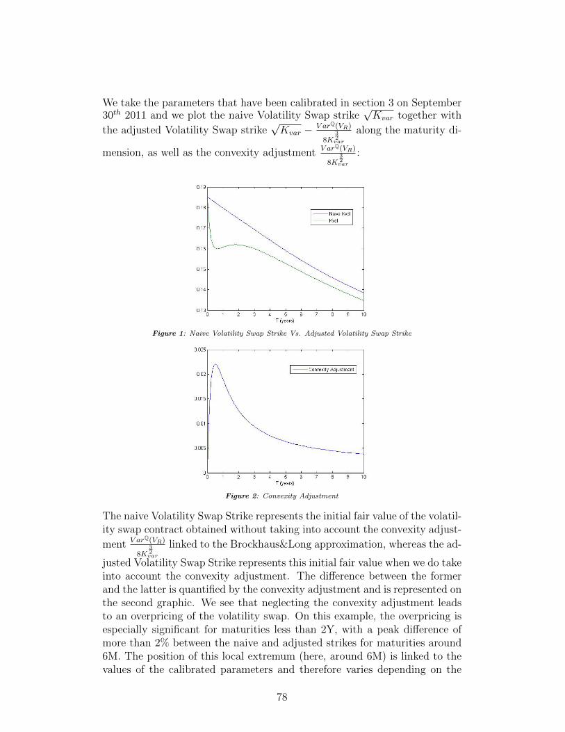
We take the parameters that have been calibrated in section 3 on September30th 2011 and we plot the naive Volatility Swap strike

√Kvar together with

the adjusted Volatility Swap strike√Kvar − V arQ(VR)

8K32var

along the maturity di-

mension, as well as the convexity adjustment V arQ(VR)

8K32var

:

Figure 1: Naive Volatility Swap Strike Vs. Adjusted Volatility Swap Strike

Figure 2: Convexity Adjustment

The naive Volatility Swap Strike represents the initial fair value of the volatil-ity swap contract obtained without taking into account the convexity adjust-

ment V arQ(VR)

8K32var

linked to the Brockhaus&Long approximation, whereas the ad-

justed Volatility Swap Strike represents this initial fair value when we do takeinto account the convexity adjustment. The difference between the formerand the latter is quantified by the convexity adjustment and is represented onthe second graphic. We see that neglecting the convexity adjustment leadsto an overpricing of the volatility swap. On this example, the overpricing isespecially significant for maturities less than 2Y, with a peak difference ofmore than 2% between the naive and adjusted strikes for maturities around6M. The position of this local extremum (here, around 6M) is linked to thevalues of the calibrated parameters and therefore varies depending on the

78

date we perform the calibration at.

We also plot the initial hedge ratio β0 along the maturity dimension:

Figure 3: Initial Hedge Ratio

This initial hedge ratio β0 represents the quantity of variance swap contractswe need to buy (if β0 > 0) or sell (if β0 < 0) to hedge our position on onevolatility swap contract of the same maturity. Of course, in order to can-cel the risk, β0 has to be negative if we buy a volatility swap contract, andpositive if we sell one. Here we have assumed that we hold a long positionon a volatility swap contract, i.e. that we have bought one such contract.The plot tells us that for one volatility swap contract bought, we need to sellapproximately 3 variance swap contracts of the same maturity (dependingof the maturity of the contract) to hedge our position on the volatility swap,i.e. to cancel the risk inherent to our position. We say that we hold a shortposition on the variance swap contracts. The trend is that the higher thematurity of the volatility swap contract, the more variance swap contractswe need to sell in order to hedge our position. This was to be expected be-cause for such pure volatility contracts, the longer the maturity, the higherthe probability that the volatility varies significantly, i.e. the higher the risk.

6 Conclusions

In this Chapter, we introduced a variance drift adjusted version of the Hes-ton model based on the concept of delay, the Delayed Heston model (section2). As explained in the introduction, this model makes a bridge between thepopular Heston model and the delayed stochastic volatility model consideredby Swishchuk in [23]. Our model has two additional parameters comparedto the Heston model and since it can be seen as a time-dependent Hestonmodel with time-dependent long-range variance θ2t , it can be implementedvery easily, for both Monte Carlo simulation and pricing of call options via

79

the semi-closed formulas which can be derived (see Appendix A). We cali-brated our model on 12 dates ranging from Sep. 19th to Oct. 17th 2011 forthe FOREX underlying EURUSD (section 3). Our findings were twofold: theDelayed Heston model always outperformed significantly the Heston modelin terms of average (absolute) calibration error (especially for long maturi-ties and ATM options), but also in terms of the standard deviation of thecalibration errors. The latter is highly desirable in practice as we do notwant to face the case of very poorly priced options on one hand, and almostperfectly priced options on the other: it is better that each individual calibra-tion error corresponding to each call option is close to the average calibrationerror, and therefore that the standard deviation of the calibration errors islow. In sections 4 and 5, we considered respectively the pricing of varianceand volatility swaps, and the dynamic hedging of a position on a volatilityswap by a position on variance swaps, the latter being very liquid financialderivatives. We obtained a closed formula for both the price process of thevariance swap and the Brockhaus&Long approximation (which is a 2nd orderapproximation) of the price process of the volatility swap. Finally, to illus-trate these last sections, we displayed 3 graphics showing the importance oftaking into account the convexity adjustment (corresponding to the Brock-haus&Long approximation) when pricing a volatility swap, and that takingnaively the volatility swap strike Kvol to be

√Kvar may lead to a significant

mispricing of the volatility swap.

A Semi-closed formulas for call options in the

Delayed Heston Model

From Kahl&Jackel [13], we get equations (71) to (74) for the price of acall option with maturity T and strike K in the time-dependent long-rangevariance Heston model:

C0 = e−rT[

1

2(F −K) +

1

π

∫ ∞0

(Fh1(u)−Kh2(u))du

], (71)

h1(u) = <(e−iu ln(K)ϕ(u− i)

iuF

), (72)

h2(u) = <(e−iu ln(K)ϕ(u)

iu

), (73)

with F = S0e(r−q)T and:

ϕ(u) = eC(T,u)+V0D(T,u)+iu ln(F ). (74)

80

By Michailov&Noegel [20], we have that C(t, u) and D(t, u) solve the follow-ing differential equations:

dC(t, u)

dt= γθ2tD(t, u), (75)

dD(t, u)

dt− δ2

2D2(t, u) + (γ − iuρδ)D(t, u) +

1

2(u2 + iu) = 0, (76)

C(0, u) = D(0, u) = 0. (77)

The Riccati equation for D(t, u) doesn’t depend on θ2t , therefore its solutionis just the solution of the classical Heston model given in Kahl&Jackel [13]:

D(t, u) =γ − iρδu+ d

δ2

[1− edt

1− gedt

], (78)

g =γ − iρδu+ d

γ − iρδu− d, (79)

d =√

(γ − iρδu)2 + δ2(iu+ u2). (80)

Given D(t, u) and the definition of θ2t , we can compute C(t, u) from (75) and(77):

C(t, u) = γθ2τf(t, u) + (V0 − θ2τ )(γ − γτ )∫ t

0

e−γτ sD(s, u)ds. (81)

Where f(t, u) =∫ t0D(s, u)ds is given in Kahl&Jackel [13]:

f(t, u) =1

δ2

((γ − iρδu+ d)t− 2 ln

(1− gedt

1− g

)). (82)

Unfortunately, the integral∫ t0e−γτ sD(s, u)ds in (81) cannot be computed

directly as∫ t0D(s, u)ds. The logarithm in f(t, u) can be handled as suggested

in Kahl&Jackel [13], as well as the integration of the Heston integral, namely:

C0 = e−rT∫ 1

0

y(x)dx, (83)

y(x) =1

2(F −K) +

Fh1(− ln(x)C∞

)−Kh2(− ln(x)C∞

)

xπC∞, (84)

81

where C∞ > 0 is an integration constant.

The following limit conditions are given in Kahl&Jackel [13]:

limx→0

y(x) =1

2(F −K), (85)

limx→1

y(x) =1

2(F −K) +

FH1 −KH2

πC∞, (86)

Hj = limu→0

hj(u) = ln

(F

K

)+ cj(T ) + V0dj(T ), (87)

where:

d1(t) = =(∂D

∂u(t,−i)

), (88)

c1(t) = =(∂C

∂u(t,−i)

), (89)

d2(t) = =(∂D

∂u(t, 0)

), (90)

c2(t) = =(∂C

∂u(t, 0)

). (91)

Expressions for d1(t) and d2(t) are the same as in Kahl&Jackel [13] as θ2tdoesn’t play any role in them. Given (75) and (77), we compute c1(T ) andc2(T ) in our time-dependent long-range variance Heston model by:

cj(T ) = γ

∫ T

0

θ2t dj(t)dt. (92)

After computing the integrals we get:

If γ − ρδ 6= 0 and γ − ρδ + γτ 6= 0:

d1(T ) =1− e−(γ−ρδ)T

2(γ − ρδ), (93)

c1(T ) = γθ2τe−(γ−ρδ)T − 1 + (γ − ρδ)T

2(γ − ρδ)2(94)

+(V0 − θ2τ )(γ − γτ )

2(γ − ρδ)

(−e−γτT − 1

γτ+e−(γ−ρδ+γτ )T − 1

γ − ρδ + γτ

). (95)

82

If γ − ρδ 6= 0 and γ − ρδ + γτ = 0:

d1(T ) =1− e−(γ−ρδ)T

2(γ − ρδ), (96)

c1(T ) = γθ2τe−(γ−ρδ)T − 1 + (γ − ρδ)T

2(γ − ρδ)2(97)

+(V0 − θ2τ )(γ − γτ )

2(γ − ρδ)

(−e−γτT − 1

γτ− T

). (98)

If γ − ρδ = 0:

d1(T ) =T

2, (99)

c1(T ) = γθ2τT 2

4+

(V0 − θ2τ )(γ − γτ )2

(−Te

−γτT

γτ+

1− e−γτT

γ2τ

), (100)

and:

d2(T ) =e−γT − 1

2γ, (101)

c2(T ) = γθ2τ1− e−γT − γT

2γ2(102)

+(V0 − θ2τ )(γ − γτ )

2γ

(−1− e−γτT

γτ− e(−γτ−γ)T − 1

γτ + γ

). (103)

References

[1] Arriojas, M., Hu, Y., Mohammed, S-E., Pap, G. A Delayed Black andScholes Formula Stochastic Analysis and Applications 25:2, 471-492, 2007.

[2] Bell, D. R., Mohammed, S-E. The Malliavin calculus and stochastic delayequations. J. Funct. Anal. 99, no. 1, 75–99, 1991.

[3] Bell, D. R., Mohammed, S-E. Smooth densities for degenerate stochasticdelay equations with hereditary drift. Ann. Probab. 23, no. 4, 1875–1894,1995.

[4] Bollerslev, T. Generalized autoregressive conditional heteroscedasticity.J. Economics 31, 307-27, 1986.

[5] Broadie, M. and Jain, A. The effect of jumps and discrete sampling onvolatility and variance swaps. Intern. J. Theor. Appl. Finance, vol. 11, no.8, pp. 761-797, 2008.

83

[6] Broadie, M and Jain, A. Pricing and Hedging Volatility Derivatives. Jour-nal of Derivatives, Vol.15, No.3, 7-24, 2008.

[7] Brockhaus, O. and Long, D. Volatility swaps made simple. Risk, January,92-96, 2000.

[8] Carr, P. and Lee, R. Volatility Derivatives. Annu. Rev, Financ. Econ.,1:1-21 (doi:10.1146/annurev.financial.050808.114304), 2009.

[9] Filipovic, D. Affine Variance Swap Curve Models. Seminar on StochasticAnalysis, Random Fields and Applications VII, Progress in Probability, 67,381-393, Springer Basel, 2013.

[10] Hao, J. and Zhang, J.E. GARCH option pricing models, the CBOEVIX, and Variance Risk premium. Journal of Financial Econometrics,11(3):556-580, 2013.

[11] Heston, S. A closed-form solution for options with stochastic volatil-ity with applications to bond and currency options. Review of FinancialStudies, 6, 327-343, 1993.

[12] Heston, S. and Nandi, S. Derivatives on volatility: some simple solutionsbased on observables. Federal Reserve Bank of Atlanta, working paper2000-20, November, 2000.

[13] Kahl, C. and Jackel, P. Not-so-complex logarithms in the Heston model.Wilmott Magazine, September, pp. 94-103, 2005.

[14] Karatzas, I. and Shreve, S.E., Brownian motion and Stochastic Calculus,2nd Edition, Springer Science+Business Media, LLC, 1998.

[15] Kazmerchuk, Y., Swishchuk, A. and Wu, J. A continuous-time GARCHmodel for stochastic volatility with delay. Candian Appl. Math. Quart., v.13, No. 2, 2005.

[16] Kazmerchuk, Y., Swishchuk, A. and Wu, J. The pricing of options forsecurity markets with delayed response. Mathematics and Computers inSimulation 75 6979, 2007.

[17] Kind, P., Lipster, R. S., Runggaldier, W. J.. Diffusion approximation inpast dependent models and applications to option pricing. The Annals ofApplied Probability vol.1, no. 3, pp. 379-405, 1991.

[18] Kruse, S. and Nogel, U. On the pricing of forward starting options inHeston’s model on stochastic volatility. Finance Stochast. 9, 233250, 2005.

[19] Mikhailov, S. and Noegel, U. Heston’s Stochastic Volatility Model Im-plementation, Calibration and Some Extensions. Wilmott Magazine, 1, pp.74-79, 2005.

84

[20] Mikhailov, S. and Noegel, U. Heston’s Stochastic Volatility Model Im-plementation, Calibration and Some Extensions. Wilmott Magazine, 1, pp.74-79, 2005.

[21] Swishchuk, A. and Li, X. Pricing variance swaps for stochastic volatili-ties with delay and jumps, Intern. J. Stoch. Anal., vol. 2011 (2011), ArticleID 435145, 2011.

[22] Swishchuk, A. Modeling of variance and volatility swaps for financialmarkets with Stochastic volatilities. Wilmott Magazine, September issue,No. 2, pp. 64-72, 2004.

[23] Swishchuk, A. Modeling and pricing of variance swaps for stochasticvolatilities with delay. Wilmott Magazine, September, No. 19, pp. 63-73,2005.

[24] Swishchuk, A. Modeling and Pricing of Variance Swaps for Multi-FactorStochastic Volatilities with Delay. Canad. Appl. Math. Quart., Volume 14,Number 4, Winter 2006.

[25] Swishchuk, A. Variance and volatility swaps in energy markets. J. En-ergy Markets, Volume 6/Number 1, Spring 2013 (3349), 2013.

[26] Swishchuk, A and Malenfant, K. Variance swap for local Levy basedstochastic volatility with delay. Intern. Rev. Appl. Fin. Iss. Econ.(IRAFIE), Vol. 3, No. 2, 2011, pp. 432-441, 2011.

[27] Swishchuk, A. and Vadori, N. Smiling for the deayaed volatility swaps.Wilmott Magazine, November 2014, 62-72.

[28] Zhang, J.E. and Zhu, Y. Vix Futures. The Journal of Futures Markets,2(6):521-531, 2006.

85

Chapter 6: CTM and Explicit Option Pricing

Formula for a Mean-reverting Asset in Energy

Markets

’Equations are more important to me, because politics is for the present,but an equation is something for eternity,’-Albert Einstein.

1 Introduction

Some commodity prices, like oil and gas, exhibit the mean reversion, unlikestock price. It means that they tend over time to return to some long-termmean. In this paper we consider a risky asset St following the mean-revertingstochastic process given by the following stochastic differential equation

dSt = a(L− St)dt+ σStdWt,

where W is a standard Wiener process, σ > 0 is the volatility, the constantL is called the ’long-term mean’ of the process, to which it reverts over time,and a > 0 measures the ’strength’ of mean reversion.

This mean-reverting model is a one-factor version of the two-factormodel made popular in the context of energy modelling by Pilipovic(1997). Black’s model (1976) and Schwartz’s model (1997) havebecome a standard approach to the problem of pricing options on com-modities. These models have the advantage of mathematical convenience,in that they give rise to closed-form solutions for some types of options (SeeWilmott (2000)).

Bos, Ware and Pavlov (2002) presented a method for evaluation ofthe price of a European option based on St, using a semi-spectral method.They did not have the convenience of a closed-form solution, however, theyshowed that values for certain types of options may nevertheless be foundextremely efficiently. They used the following partial differential equation(see, for example, Wilmott, Howison and Dewynne (1995))

C ′t +R(S, t)C ′S + σ2S2C ′′SS/2 = rC

for option prices C(S, t), where R(S, t) depends only on S and t, and corre-sponds to the drift induced by the risk-neutral measure, and r is the risk-freeinterest rate. Simplifying this equation to the singular diffusion equationthey were able to calculate numerically the solution.

The aim of this paper is to obtain an explicit expression for a Euro-pean option price, C(S, t), based on St, using a change of time method (seeSwishchuk (2007)). This method was once applied by the author to pricevariance, volatility, covariance and correlation swaps for the Heston model(see Swishchuk (2004)).

86

2 Mean-Reverting Asset Model (MRAM)

Let (Ω,F ,Ft, P ) be a probability space with a sample space Ω, σ-algebraof Borel sets F and probability P. The filtration Ft, t ∈ [0, T ], is thenatural filtration of a standard Brownian motion Wt, t ∈ [0, T ], such thatFT = F .

Some commodity prices, like oil and gas, exhibit the mean reversion,unlike stock price. It means that they tend over time to return to some long-term mean. In this paper we consider a risky asset St following the mean-reverting stochastic process given by the following stochastic differentialequation

dSt = a(L− St)dt+ σStdWt, (1)

where Wt is an Ft-measurable one-dimensional standard Wiener process,σ > 0 is the volatility, constant L is called the ’long-term mean’ of theprocess, to which it reverts over time, and a > 0 measures the ’strength’ ofmean reversion.

3 Explicit Option Pricing Formula for Euro-

pean Call Option for MRAM under Phys-

ical Measure

In this section, we are going to obtain an explicit expression for a Euro-pean option price, C(S, t), based on St, using a change of time method andphysical measure.

3.1 Explicit Solution of MRAM.

Let

Vt := eat(St − L). (2)

Then, from (2) and (1) we obtain

dVt = aeat(St − L)dt+ eatdSt = σ(Vt + eatL)dWt. (3)

Using change of time approach to the equation (3) (see Ikeda andWatanabe (1981) or Elliott (1982)) we obtain the following solutionof the equation (3)

Vt = S0 − L+ W (φ−1t ),

or (see (2)),

St = e−at[S0 − L+ W (φ−1t )] + L, (4)

87

where W (t) is an Ft-measurable standard one-dimensional Wiener process,φ−1t is an inverse function to φt :

φt = σ−2∫ t

0

(S0 − L+ W (s) + eaφsL)−2ds. (5)

We note that

φ−1t = σ2

∫ t

0

(S0 − L+ W (φ−1t ) + easL)2ds, (6)

which follows from (5) and the following transformations:

dφt = σ−2(S0−L+W (t)+eaφtL)−2dt⇒ σ2(S0−L+W (t)+eaφtL)2dφt = dt⇒

t = σ2∫ t0(S0 − L+ W (s) + eaφsL)2dφs ⇒

φ−1t = σ2∫ φ−1

t

0(S0 − L+ W (s) + eaφsL)2dφs

= σ2∫ t0(S0 − L+ W (φ−1s ) + easL)2ds.

3.2 Some Properties of the Process W (φ−1t ).

We note that process W (φ−1t ) is Ft := Fφ−1t

-measurable and Ft-martingale.

Then

EW (φ−1t ) = 0. (7)

Let’s calculate the second moment of W (φ−1t ) (see (6)):

EW 2(φ−1t ) = E < W (φ−1t ) >= Eφ−1t= σ2

∫ t0E(S0 − L+ W (φ−1s ) + easL)2ds

= σ2[(S0 − L)2t+ 2L(S0−L)(eat−1)a

+ L2(e2at−1)2a

+∫ t0EW 2(φ−1s )ds].

(8)

From (8), solving this linear ordinary nonhomogeneous differential equationwith respect to EW 2(φ−1t ),

dEW 2(φ−1t )

dt= σ2[(S0 − L)2 + 2L(S0 − L)eat + L2e2at + EW 2(φ−1t )],

we obtain

EW 2(φ−1t ) = σ2[(S0−L)2eσ

2t − 1

σ2+

2L(S0 − L)(eat − eσ2t)

a− σ2+L2(e2at − eσ2t)

2a− σ2].

(9)

88

3.3 Explicit Expression for the Process W (φ−1t ).

It is turns out that we can find the explicit expression for the processW (φ−1t ).

From the expression (see Section 3.1)

Vt = S0 − L+ W (φ−1t ),

we have the following relationship between W (t) and W (φ−1t ) :

dW (φ−1t ) = σ

∫ t

0

[S(0)− L+ Leat + W (φ−1s )]dW (t).

It is a linear SDE with respect to W (φ−1t ) and we can solve it explicitly.The solution has the following look:

W (φ−1t ) = S(0)(eσW (t)−σ2t2 −1)+L(1−eat)+aLeσW (t)−σ

2t2

∫ t

0

ease−σW (s)+σ2s2 ds.

(10)It is easy to see from (10) that W (φ−1t ) can be presented in the form of

a linear combination of two zero-mean martingales m1(t) and m2(t) :

W (φ−1t ) = m1(t) + Lm2(t),

where

m1(t) := S(0)(eσW (t)−σ2t2 − 1)

and

m2(t) = (1− eat) + aeσW (t)−σ2t2

∫ t

0

ease−σW (s)+σ2s2 ds.

Indeed, process W (φ−1t ) is a martingale (see Section 3.2), also it is well-

known that process eσW (t)−σ2t2 and, hence, process m1(t) is a martingale.

Then the process m2(t), as the difference between two martingales, is alsomartingale. In this way, we have

Em1(t) = 0,

since

EeσW (t)−σ2t2 = 1.

As for m2(t) we haveEm2(t) = 0,

since from Ito’s formula we have

d(aeσW (t)−σ2t2

∫ t0ease−σW (s)+σ2s

2 ds) = aσeσW (t)−σ2t2

∫ t0ease−σW (s)+σ2s

2 dsdW (t)

+ aeσW (t)−σ2t2 eate−σW (t)+σ2t

2 dt

= aσeσW (t)−σ2t2

∫ t0ease−σW (s)+σ2s

2 dsdW (t)+ aeatdt,

89

and, hence,

EaeσW (t)−σ2t2

∫ t

0

ease−σW (s)+σ2s2 ds = eat − 1.

It is interesting to see that the last expression, the first moment for

η(t) := aeσW (t)−σ2t2

∫ t

0

ease−σW (s)+σ2s2 ds,

does not depend on σ.It is true not only for the first moment but for all the moments of the

process η(t) = aeσW (t)−σ2t2

∫ t0ease−σW (s)+σ2s

2 ds.Indeed, using Ito’s formula for ηn(t) we obtain

dηn(t) = nanσenσW (t)−nσ2t2 (

∫ t0ease−σW (s)+σ2s

2 ds)ndW (t) + an(η2(t))n−1eatdt,

anddEηn(t) = naeatEηn−1(t)dt, n ≥ 1.

This is a recursive equation with initial function (n = 1) Eη(t) = eat − 1.After calculations we obtain the following formula for Eηn(t) :

Eηn(t) = (eat − 1)n.

3.4 Some Properties of the Mean-Reverting Asset St

From (4) we obtain the mean value of the first moment for mean-revertingasset St :

ESt = e−at[S0 − L] + L.

It means that ESt → L when t→ +∞.Using formulae (4) and (9) we can calculate the second moment of St :

ES2t = (e−at(S0 − L) + L)2

+ σ2e−2at[(S0 − L)2 eσ2t−1σ2 + 2L(S0−L)(eat−eσ

2t)a−σ2 + L2(e2at−eσ2t)

2a−σ2 ].

Combining the first and the second moments we have the variance ofSt :

V ar(St) = ES2t − (ESt)

2

= σ2e−2at[(S0 − L)2 eσ2t−1σ2 + 2L(S0−L)(eat−eσ

2t)a−σ2 + L2(e2at−eσ2t)

2a−σ2 ].

From the expression for W (φ−1t ) (see (10)) and for S(t) in (4) we canfind the explicit expression for S(t) through W (t) :

90

S(t) = e−at[S0 − L+ W (φ−1t )] + L= e−at[S0 − L+m1(t) + Lm2(t)] + L

= S(0)e−ateσW (t)−σ2t2 + aLe−ateσW (t)−σ

2t2

∫ t0ease−σW (s)+σ2s

2 ds,(11)

where m1(t) and m2(t) are defined as in Section 3.3.

3.5 Explicit Option Pricing Formula for European CallOption for MRAM under Physical Measure.

The payoff function fT for European call option equals

fT = (ST −K)+ := max(ST −K, 0),

where ST is an asset price defined in (4), T is an expiration time (maturity)and K is a strike price.

In this way (see (11)),

fT = [e−aT (S0 − L+ W (φ−1T )) + L−K]+

= [S(0)e−aT eσW (T )−σ2T2 + aLe−aT eσW (T )−σ

2T2

∫ T0ease−σW (s)+σ2s

2 ds−K]+.

To find the option pricing formula we need to calculate

CT = e−rTEfT= e−rTE[e−aT (S0 − L+ W (φ−1T )) + L−K]+

= 1√2πe−rT

∫ +∞−∞ max[S(0)e−aT eσy

√T−σ

2T2

+ aLe−aT eσy√T−σ

2T2

∫ T0ease−σy

√s+σ2s

2 ds−K, 0]e−y2

2 dy.

(12)

Let y0 be a solution of the following equation:

S(0) × e−aT eσy0√T−σ

2T2

+ aLe−aT eσy0√T−σ

2T2

∫ T0ease−σy0

√s+σ2s

2 ds = K(13)

or

y0 =ln( K

S(0)) + (σ

2

2+ a)T

σ√T

−ln(1 + aL

S(0)

∫ T0ease−σy0

√s+σ2s

2 ds)

σ√T

(14)

91

From (12)-(13) we have:

CT = 1√2πe−rT

∫ +∞−∞ max[S(0)e−aT eσy

√T−σ

2T2

+ aLe−aT eσy√T−σ

2T2

∫ T0ease−σy

√s+σ2s

2 ds−K, 0]e−y2

2 dy

= 1√2πe−rT

∫ +∞y0

[S(0)e−aT eσy√T−σ

2T2

+ aLe−aT eσy√T−σ

2T2

∫ T0ease−σy

√s+σ2s

2 ds−K]e−y2

2 dy

= 1√2πe−rT

∫ +∞y0

[S(0)e−aT eσy√T−σ

2T2 e−

y2

2 dy − e−rTK[1− Φ(y0)]

+ Le−(r+a)T 1√2π

∫ +∞y0

(aeσy√T−σ

2T2

∫ T0ease−σy

√s+σ2s

2 ds)e−y2

2 dy

= BS(T ) + A(T ),(15)

where

BS(T ) :=1√2πe−rT

∫ +∞

y0

[S(0)e−aT eσy√T−σ

2T2 e−

y2

2 dy − e−rTK[1− Φ(y0)],

(16)A(T ) := Le−(r+a)T

× 1√2π

∫ +∞y0

(aeσy√T−σ

2T2

∫ T0ease−σy

√s+σ2s

2 ds)e−y2

2 dy,(17)

and

Φ(x) =1√2π

∫ x

−∞e−

y2

2 dy. (18)

After calculation of BS(T ) we obtain

BS(T ) = e−(r+a)TS(0)Φ(y+)− e−rTKΦ(y−), (19)

wherey+ := σ

√T − y0 and y− := −y0 (20)

and y0 is defined in (14).Consider A(T ) in (17).Let FT (dz) be a distribution function for the process

η(T ) = aeσW (T )−σ2T2

∫ T

0

ease−σW (s)+σ2s2 ds,

which is a part of the integrand in (17).As M. Yor [16, 17] mentioned there is still no closed form probability

density function for time integral of an exponential Brownian motion, whilethe best result is a function with a double integral.

We can use Yor’s result [16] to get FT (dz) above. Using the scalingproperty of Wiener process and change of variables, we can rewrite ourexpression for S(t) in (11) in the following way

S(T ) = S(0)e−2BvT0 +

4

σ2aLe−2B

vT0AvT0 ,

92

where T0 = σ2

4T, v = 2

σ2a + 1, Bt = −σ2W ( 4

σ2 t), BvT0

= vT0 + BT0 , AvT0

=∫ T00e2B

vs ds.

Also, the process η(T ) may be presented in the following way using thesetransformations

η(T ) =4ae−aT

σ2e−2Bσ2T

4 Aσ2T4

.

We state here the result obtained by Yor [16] for the joint probabilitydensity function of AvT0 and Bv

T0.

Theorem 4.3.-1. (M. Yor [15]). The joint probability density functionof AvT0 and Bv

T0satisfies

P (AvT0 ∈ du,BvT0∈ dx) = evx−v

2t/2 exp−1 + e2x

2uθ(ex

u, t)dxdu

u,

where t > 0, u > 0, x ∈ R and

θ(r, t) =r

(2π3t)1/2eπ2

2t

∫ +∞

0

e−s2

2t−r cosh s sinh(s) sin(

πs

t)ds.

Using this result we can write the distribution function for η(T ) in thefollowing way

P (η(T ) ≤ u) = P (4ae−aT

σ2 e−2Bσ2T

4 Aσ2T4

≤ u)

= P (e−2Bσ2T

4 Aσ2T4

≤ σ2eaT

4au)

= FT (u).

(21)

In this way, A(T ) in (17) may be presented in the following way:

A(T ) = Le−(r+a)T∫ +∞

y0

zFT (dz).

After calculation of A(T ) we obtain the following expression for A(T ) :

A(T ) = Le−(r+a)T [(eaT − 1)−∫ y0

0

zFT (dz)],

since Eη(T ) = eaT − 1.Finally, summarizing (12)-(21), we have obtained the following Theorem.

Theorem 3.1. Option pricing formula for European call option for mean-reverting asset under physical measure has the following look:

CT = e−(r+a)TS(0)Φ(y+)− e−rTKΦ(y−)+ Le−(r+a)T [(eaT − 1)−

∫ y00zFT (dz)],

(22)

where y0 is defined in (14), y+ and y− in (20), Φ(y) in (18), and FT (dz) isa distribution function in (21).

93

Remark. From (21)-(22) we find that European Call Option Price CT formean-reverting asset lies between the following boundaries:

BS(T ) ≤ CT ≤ BS(T ) + Le−(r+a)T [eaT − 1],

or (see (19)),

e−(r+a)TS(0)Φ(y+)− e−rTKΦ(y−) ≤ CT≤ e−(r+a)TS(0)Φ(y+)− e−rTKΦ(y−) + Le−(r+a)T [eaT − 1].

4 Mean-Reverting Risk-Neutral Asset Model

(MRRNAM)

Consider our model (1)

dSt = a(L− St)dt+ σStdWt. (23)

We want to find a probability P ∗ equivalent to P, under which theprocess e−rtSt is a martingale, where r > 0 is a constant interest rate. Thehypothesis we made on the filtration (Ft)t∈[0,T ] allows us to express thedensity of the probability P ∗ with respect to P. We denote this density byLT .

It is well-known (see Lamperton and Lapeyre (1996), Proposition6.1.1, p. 123), that there is an adopted process (q(t))t∈[0,T ] such that, for allt ∈ [0, T ],

Lt = exp[

∫ t

0

q(s)dWs −1

2

∫ t

0

q2(s)ds] a.s.

In this case,

dP ∗

dP= exp[

∫ T

0

q(s)dWs −1

2

∫ T

0

q2(s)ds] = LT .

In our case, with model (17), the process q(t) is equal to

q(t) = −λSt, (24)

where λ is the market price of risk and λ ∈ R. Hence, for our model

LT = exp[−λ∫ T

0

S(u)dWu −1

2λ

∫ T

0

S2(u)du].

94

Under probability P ∗, the process (W ∗t ) defined by

W ∗t := Wt + λ

∫ t

0

S(u)du (25)

is a standard Brownian motion (Girsanov theorem) (see Elliott andKopp (1999)).

Therefore, in a risk-neutral world our model (23) takes the followinglook:

dSt = (aL− (a+ λσ)St)dt+ σStdW∗t ,

or, equivalently,dSt = a∗(L∗ − St)dt+ σStdW

∗t , (26)

where

a∗ := a+ λσ, L∗ :=aL

a+ λσ, (27)

and W ∗t is defined in (25).

Now, we have the same model in (26) as in (1), and we are going to applyour method of changing of time to this model (26) to obtain the explicitoption pricing formula.

5 Explicit Option Pricing Formula for Euro-

pean Call Option for MRRNAM

In this section, we are going to obtain explicit option pricing formula forEuropean call option under risk-neutral measure P ∗, using the same argu-ments as in sections 3-7, where in place of a and L we are going to take a∗

and L∗

a→ a∗ := a+ λσ, L→ L∗ :=aL

a+ λσ,

where λ is a market price of risk (See section 3).

5.1 Explicit Solution for the Mean-Reverting Risk-Neutral Asset Model.

Applying (2)-(6) to our model (26) we obtain the following explicit solutionfor our risk-neutral model (26):

St = e−a∗t[S0 − L∗ + W ∗((φ∗t )

−1)] + L, (28)

where W ∗(t) is an Ft-measurable standard one-dimensional Wiener processunder measure P ∗ and (φ∗t )

−1 is an inverse function to φ∗t :

φ∗t = σ−2∫ t

0

(S0 − L∗ + W ∗(s) + ea∗φ∗sL∗)−2ds. (29)

95

We note that

(φ∗)−1t = σ2

∫ t

0

(S0 − L∗ + W ∗((φ∗t )−1) + ea

∗sL∗)2ds, (30)

where a∗ and L∗ are defined in (27).

5.2 Some Properties of the Process W ∗((φ∗t )−1).

Using the same argument as in Section 4, we obtain the following propertiesof the process W ∗((φ∗t )

−1) in (25). This is a zero-mean P ∗-martingale and

E∗W ∗((φ∗t )−1) = 0,

E∗[W ∗((φ∗t )−1)]2 = σ2[(S0 − L∗)2 e

σ2t−1σ2 + 2L∗(S0−L∗)(ea

∗t−eσ2t)a∗−σ2

+ (L∗)2(e2a∗t−eσ2t)

2a∗−σ2 ],

(31)

where E∗ is the expectation with respect to the probability P ∗ and a∗, L∗

and (φ∗t )−1 are defined in (27) and (30), respectively.

5.3 Explicit Expression for the Process W ∗(φ−1t ).

It is turns out that we can find the explicit expression for the processW ∗(φ−1t ).

From the expression

Vt = S0 − L+ W ∗(φ−1t ),

we have the following relationship between W (t) and W (φ−1t ) :

dW ∗(φ−1t ) = σ

∫ t

0

[S(0)− L+ Leat + W ∗(φ−1s )]dW ∗(t).

It is linear SDE with respect to W ∗(φ−1t ) and we can solve it explicitly. Thesolution has the following look:

W ∗(φ−1t ) = S(0)(eσW∗(t)−σ

2t2 − 1) + L(1− eat)

+ aLeσW∗(t)−σ

2t2

∫ t0ease−σW

∗(s)+σ2s2 ds.

(32)

It is easy to see from (32) that W ∗(φ−1t ) can be presented in the form ofa linear combination of two zero-mean P ∗-martingales m∗1(t) and m∗2(t) :

W ∗(φ−1t ) = m∗1(t) + L∗m∗2(t),

where

m∗1(t) := S(0)(eσW∗(t)−σ

2t2 − 1)

96

and

m∗2(t) = (1− ea∗t) + a∗eσW∗(t)−σ

2t2

∫ t

0

ea∗se−σW

∗(s)+σ2s2 ds.

Indeed, process W ∗(φ−1t ) is a martingale (see Section 5.2), also it is well-

known that process eσW∗(t)−σ

2t2 and, hence, process m∗1(t) is a martingale.

Then the process m∗2(t), as the difference between two martingales, is alsomartingale. In this way, we have

EP ∗m∗1(t) = 0,

since

EP ∗eσW∗(t)−σ

2t2 = 1.

As for m2(t) we haveEP ∗m2(t) = 0,

since from Ito’s formula we have

d (a∗eσW∗(t)−σ

2t2

∫ t0ea

∗se−σW∗(s)+σ2s

2 ds)

= a∗σeσW∗(t)−σ

2t2

∫ t0ea

∗se−σW∗(s)+σ2s

2 dsdW ∗(t)

+ a∗eσW∗(t)−σ

2t2 ea

∗te−σW∗(t)+σ2t

2 dt

= a∗σeσW∗(t)−σ

2t2

∫ t0ea

∗se−σW∗(s)+σ2s

2 dsdW ∗(t)+ a∗ea

∗tdt,

and, hence,

EP ∗a∗eσW∗(t)−σ

2t2

∫ t

0

ea∗se−σW

∗(s)+σ2s2 ds = ea

∗t − 1.

It is interesting to see that in the last expression, the first moment for

η∗(t) := a∗eσW∗(t)−σ

2t2

∫ t

0

ea∗se−σW

∗(s)+σ2s2 ds,

does not depend on σ.This is true not only for the first moment but for all the moments of the

process η∗(t) = a∗eσW∗(t)−σ

2t2

∫ t0ea

∗se−σW∗(s)+σ2s

2 ds.Indeed, using the Ito’s formula for (η∗(t))n we obtain

d(η∗(t))n = n(a∗)nσenσW∗(t)−nσ

2t2 (

∫ t0ea

∗se−σW∗(s)+σ2s

2 ds)ndW ∗(t)+ a∗n(η2(t))

n−1ea∗tdt,

anddE(η∗(t))n = na∗ea

∗tE(η∗(t))n−1dt, n ≥ 1.

This is a recursive equation with initial function (n = 1) Eη∗(t) = ea∗t − 1.

After calculations we obtain the following formula for E(η∗(t))n :

E(η∗(t))n = (ea∗t − 1)n.

97

5.4 Some Properties of the Mean-Reverting Risk-NeutralAsset St.

Using the same argument as in Section 5, we obtain the following propertiesof the mean-reverting risk-neutral asset St in (18):

E∗St = e−a∗t[S0 − L∗] + L∗

V ar∗(St) := E∗S2t − (E∗St)

2

= σ2e−2a∗t[(S0 − L∗)2 e

σ2t−1σ2 + 2L∗(S0−L∗)(ea

∗t−eσ2t)a∗−σ2

+ (L∗)2(e2a∗t−eσ2t)

2a∗−σ2 ],

(33)

where E∗ is the expectation with respect to the probability P ∗ and a∗, L∗

and (φ∗t )−1 are defined in (27) and (30), respectively.

From the expression for W ∗(φ−1t ) (see (32)) and for S(t) in (28) (see also(29)-(30)) we can find the explicit expression for S(t) through W ∗(t) :

S(t) = e−a∗t[S0 − L∗ + W ∗(φ−1t )] + L∗

= e−a∗t[S0 − L∗ +m∗1(t) + L∗m∗2(t)] + L∗

= S(0)e−ateσW∗(t)−σ

2t2 + aLe−ateσW

∗(t)−σ2t2

∫ t0ease−σW

∗(s)+σ2s2 ds,

(34)where m∗1(t) and m∗2(t) are defined as in section 5.3.

5.5 Explicit Option Pricing Formula for European CallOption for MRAM under Risk-Neutral Measure.

Proceeding with the same calculations (15)-(22) as in Section 3, where inplace of a and L we take a∗ and L∗ in (27), we obtain the following Theorem.Theorem 5.1. Explicit option pricing formula for European call optionunder risk-neutral measure has the following look:

C∗T = e−(r+a∗)TS(0)Φ(y+)− e−rTKΦ(y−)

+ L∗e−(r+a∗)T [(ea

∗T − 1)−∫ y00zF ∗T (dz)],

(35)

where y0 is the solution of the following equation

y0 =ln( K

S(0)) + (σ

2

2+ a∗)T

σ√T

−ln(1 + a∗L∗

S(0)

∫ T0ea

∗se−σy0√s+σ2s

2 ds)

σ√T

, (36)

y+ := σ√T − y0 and y− := −y0, (37)

98

a∗ := a+ λσ, L∗ :=aL

a+ λσ,

and F ∗T (dz) is the probability distribution as in (21), where instead of a wehave to take a∗ = a+ λσ.Remark. From (35) we can find that European Call Option Price C∗T formean-reverting asset under risk-neutral measure lies between the followingboundaries:

e−(r+a∗)TS(0)Φ(y+)− e−rTKΦ(y−) ≤ CT

≤ e−(r+a∗)TS(0)Φ(y+)− e−rTKΦ(y−)

+ L∗e−(r+a∗)T [ea

∗T − 1],(38)

where y0, y−, y+ are defined in (36)-(37).

5.6 Black-Scholes Formula Follows: L∗ = 0 and a∗ =−r.

If L∗ = 0 and a∗ = −r we obtain from (35)

CT = S(0)Φ(y+)− e−rTKΦ(y−), (39)

wherey+ := σ

√T − y0 and y− := −y0, (40)

and y0 is the solution of the following equation (see (36))

S(0)e−rT eσy0√T−σ

2T2 = K

or

y0 =ln( K

S(0)) + (σ

2

2− r)T

σ√T

. (41)

But (39)-(41) is exactly the well-known Black-Scholes result!

6 Numerical Example: AECO Natural GAS

Index (1 May 1998-30 April 1999)

We shall calculate the value of a European call option on the price of adaily natural gas contract. To apply our formula for calculating this valuewe need to calibrate the parameters a, L, σ and λ. These parametersmay be obtained from futures prices for the AECO Natural Gas Index forthe period 1 May 1998 to 30 April 1999 (see Bos, Ware and Pavlov(2002), p.340). The parameters pertaining to the option are the following:

99

Price and Option Process ParametersT a σ L λ r K6months

4.6488 1.5116 2.7264 0.1885 0.05 3

From this table we can calculate the values for a∗ and L∗ :

a∗ = a+ λσ = 4.9337,

and

L∗ =aL

a+ λσ= 2.5690.

For the value of S0 we can take S0 ∈ [1, 6].Figure 1 (see Appendix) depicts the dependence of mean value ESt on

the maturity T for AECO Natural Gas Index (1 May 1998 to 30 April 1999).Figure 2 (see Appendix) depicts the dependence of mean value ESt on

the initial value of stock S0 and maturity T for AECO Natural Gas Index(1 May 1998 to 30 April 1999).

Figure 3 (see Appendix) depicts the dependence of variance of St on theinitial value of stock S0 and maturity T for AECO Natural Gas Index (1May 1998 to 30 April 1999).

Figure 4 (see Appendix) depicts the dependence of volatility of St onthe initial value of stock S0 and maturity T for AECO Natural Gas Index(1 May 1998 to 30 April 1999).

Figure 5 (see Appendix) depicts the dependence of European Call OptionPrice for MRRNAM on the maturity (months) for AECO Natural Gas Index(1 May 1998 to 30 April 1999) with S(0) = 1 and K = 3.

Appendix: Figures

100

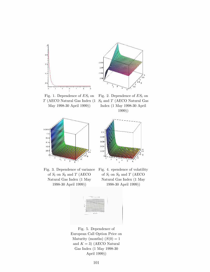
Fig. 1. Dependence of ESt on

T (AECO Natural Gas Index (1

May 1998-30 April 1999))

Fig. 2. Dependence of ESt on

S0 and T (AECO Natural Gas

Index (1 May 1998-30 April

1999))

Fig. 3. Dependence of variance

of St on S0 and T (AECO

Natural Gas Index (1 May

1998-30 April 1999))

Fig. 4. ependence of volatility

of St on S0 and T (AECO

Natural Gas Index (1 May

1998-30 April 1999))

Fig. 5. Dependence of

European Call Option Price on

Maturity (months) (S(0) = 1

and K = 3) (AECO Natural

Gas Index (1 May 1998-30

April 1999))

101

References

1. Bos, L. P., Ware, A. F. and Pavlov, B. S. (2002) On a semi-spectral methodfor pricing an option on a mean-reverting asset, Quantitative Finance, 2,337-345.

2. Black, F. (1076) The pricing of commodity contracts, J. Financial Eco-nomics, 3, 167-179.

3. Chen, Z. and Forsyth, P. (2006) Stochastic models of natural gas prices andapplications to natural gas storage valuation, Technical Report, Universityof Waterloo, Waterloo, Canada, November 24, 32p.(http://www.cs.uwaterloo.ca/ paforsyt/regimestorage.pdf).

4. Elliott, R. (1982) Stochastic Calculus and Applications, Springer-Verlag,New York.

5. Elliott, R. and Kopp, E. (1999) Mathematics of Financial Markets, Springer-Verlag, New York.

6. Ikeda, N. and Watanabe, S. (1981) Stochastic Differential Equations andDiffusion Processes, Kodansha Ltd., Tokyo.

7. Lamperton, D. and Lapeyre, B. (1996) Introduction to Stochastic CalculusApplied to Finance, Chapmann & Hall.

8. Pilipovic, D. (1997) Valuing and Managing Energy Derivatives, New York,McGraw-Hill.

9. Schoutens, W. (2003 Levy Processes in Finance: Pricing Financial Deriva-tives, Wiley.

10. Schwartz, E. (1997) The stochastic behaviour of commodity prices: impli-cations for pricing and hedging, J. Finance, 52, 923-973.

11. Swishchuk, A. (2004) Modeling and valuing of variance and volatility swapsfor financial markets with stochastic volatilities, Wilmott Magazine, Tech-nical Article No2, September Issue, 64-72.

12. Swishchuk, A. (2007) Change of time method in mathematical finance,CAMQ, Vol. 15, No. 3, 299-336.

13. Swishchuk A.. (2008) Explicit option pricing formula for a mean-revertingasset in energy market. Journal of Numerical and Applied Mathematics.1(96): 23.

14. Wilmott, P., Howison, S. and Dewynne, J. (1995) The Mathematics ofFinancial Derivatives, Cambridge, Cambridge University Press.

15. Wilmott, P. (2000) Paul Wilmott on Quantitative Finance, New York, Wi-ley.

16. Yor, M. (1992) On some exponential functions of Brownian motion, Ad-vances in Applied Probability, Vol. 24, No. 3, 509-531.

17. Yor, M. and Matsumoto, H. (2005) Exponential Functionals of Brownian

motion, I: Probability laws at fixed time, Probability Surveys, Vol. 2, 312-

347.

102

Chapter 7: CTM and Multi-Factor Levy

Models for Pricing Financial and Energy

Derivatives

’The energy of the mind is the essence of life’,-Aristotle.

1 Introduction

In this chapter, we introduce one-factor and multi-factor α-stable Levy-basedmodels to price financial and energy derivatives. These models include, inparticular, as one-factor models, the Levy-based geometric motion model,the Ornstein-Uhlenbeck (1930), the Vasicek (1977), the Cox-Ingersoll-Ross(1985), the continuous-time GARCH, the Ho-Lee (1986), the Hull-White(1990) and the Heath-Jarrrow-Morton (1992) models, and, as multi-factormodels, various combinations of the previous models. For example, we in-troduce new multi-factor models such as the Levy-based Heston model, theLevy-based SABR/LIBOR market models, and Levy-based Schwartz-Smithand Schwartz models. Using the change of time method for SDEs driven byα-stable Levy processes we present the solutions of these equations in sim-ple and compact forms. We then apply this method to price many financialand energy derivatives such as variance swaps, options, forward and futurescontracts.

In this first section, we first review in brief literature on the change of timemethod (CTM) for Levy-based models, and give an overview of the multi-factor Gaussian, LIBOR and SABR models, swaps and energy derivatives.

1.1 Change of Time Method (CTM) for Levy-basedModels: Short Literature History

Rosinski & Woyczynski (1986) considered time changes for integrals over astable Levy processes. Kallenberg (1992) considered time change represen-tations for stable integrals.

Levy processes can also be used as a time change for other Levy processes(subordinators). Madan & Seneta (1990) introduced Variance Gamma (VG)process (Brownian motion with drift time changed by a gamma process).Geman, Madan & Yor (2001) considered time changes (’business times’) forLevy processes . Carr, Geman, Madan & Yor (2003) used a change of timeto introduce stochastic volatility into a Levy model to achieve leverage effectand a long-term skew. Kallsen & Shiryaev (2001) showed that the Rosinski-Woyczynski-Kallenberg result can not be extended to any other Levy pro-cesses other than the symmetric α-stable processes. Swishchuk (2004, 2007)applied a change of time method for options and swaps pricing for Gaussianmodels.

103

The book ’Change of Time and Change of Measure’ by Barndorff-Nielsenand Shiryaev (2010) states the main ideas and results of the stochastic theoryof ’change of time and change of measure’ in the semimartingale setting.

1.2 Stochastic Differential Equations (SDEs) Drivenby Levy Processes

Girsanov (1960) used the change of time method to construct a weak solutionto a specific SDE driven by Brownian motion.

The existence and uniqueness of solutions for SDEs driven by Levy pro-cesses have been studied in Applebaum (2003). The existence and uniquenessof solutions for SDEs driven by general semimartingale with jumps have beenstudied in Protter (2005) and Jacod (1979).

Janicki, Michna & Weron (1996) proved that there exists a unique solutionof the SDE for continuous drift b and diffusion coefficient σ and α-stable Levyprocess Sα((t− s)1/α, β, δ), β ∈ [−1,+1].

Zanzotto (1997) had also considered solutions of one-dimensional SDEsdriven by stable Levy motion.

Cartea & Howison (2006) considered option pricing with Levy-stable pro-cesses generated by Levy-stable integrated variance.

1.3 Multi-Factor Gaussian Models: Literature Review

Eydeland and Geman (1998) proposed extending the Heston (1993) stochas-tic volatility model to gas or electricity prices by introducing mean-reversionin the spot price and leaving the CIR model for the variance, resulting in atwo-state variable model for commodity prices.

Geman (2000) proposed a three-state variable for oil prices by introducingmean-reversion in the spot price, geometric Brownian motion in the equilib-rium (or mean-reverting) price and the CIR model in the variance.

Gibson and Schwartz (1990) note that the convenience yield has beenshown to be a key factor driving the relationship between spot and futuresprices, and they proposed the two-state variable model for oil-contingentclaim pricing.

Continuing to the more complex level of two factor models, keeping thesame mean-reverting level Lt, the SDEs for spot price St and Lt can be gen-eralized by either allowing the long run mean Lt or the volatility σ to begoverned by an SDE. This leads to two distinct two factor models, with dif-ferent dynamics. The first model assumes a stochastic long run mean andwas introduced by Pilipovic (1997). Pilipovic (1997) describes a two-factormean-reverting model where spot prices revert to a long term equilibriumlevel which is itself a random variable. Pilipovich derives a closed-form solu-tion for forward prices to her model when the spot and long term prices areuncorrelated, but does not discuss option pricing in her two-factor model.

104

Gibson and Schwartz (1990), Schwartz (1997) and Hilliard and Reis (1998)all analyze versions of the same two-factor model that allows for a stochasticconvenience yield and permits a high level of analytical tractability. Thefirst factor is the spot price process which is assumed to follow the geometricBrownian motion (GBM) and the second factor is the instantaneous conve-nience yield of the spot energy and is assumed to follow the mean revertingprocess.

Schwartz (1997) extends his two-factor model to include stochastic inter-est rates. In this three-factor model the short term rate is assumed to followthe Vasicek (1977) mean-reverting process.

Fouque, Papanicolaou and Sircar (2000) considered multi-factor stochas-tic volatility model that is a function of two processes in the form of geometricBrownian motions.

Fouque and Han (2003) found that two-factor SV models provide a betterfit to the term structure of implied volatility than one factor SV models bycapturing the behavior at short and long maturities.

Chernov et al (2003) used two-factor SV family models to obtain compa-rable empirical goodness-of-fit.

Molina et al (2003) found a strong evidence of two-factor SV models withwell-separated time scales in foreign exchange data.

Carmona and Ludkovski (2003) reviewed the literature of spot conve-nience yield models, and analyzed in detail two new extensions. First, theydiscussed a variant of the Gibson-Schwartz model with time-dependent pa-rameters and second, they described a new three-factor affine model withstochastic convenience yield and stochastic market price of risk.

1.4 Pricing Swaps Overview

Demeterfi, K., Derman, E., Kamal, M., and Zou, J. (1999) explained theproperties and the theory of both variance and volatility swaps. They derivedan analytical formula for the theoretical fair value in the presence of realisticvolatility skews, and pointed out that volatility swaps can be replicated bydynamically trading the more straightforward variance swap.

Javaheri A, Wilmott, P. and Haug, E. G. (2002) discussed the valuationand hedging of a GARCH(1,1) stochastic volatility model. They used ageneral and flexible PDE approach to determine the first two moments of therealized variance in a continuous or discrete context. Then they approximatethe expected realized volatility via a convexity adjustment.

Working paper by Theoret, Zabre and Rostan (2002) presented an ana-lytical solution for pricing of volatility swaps, proposed by Javaheri, Wilmottand Haug (2002). They priced volatility swaps within framework of GARCH(1,1)stochastic volatility model and applied the analytical solution to price aswap on volatility of the S&P60 Canada Index (5-year historical period:1997− 2002).

105

Brockhaus and Long (2000) provided an analytical approximation forthe valuation of volatility swaps and analyzed other options with volatilityexposure.

In Swishchuk (2004) we found the values of variance and volatility swapsfor financial markets with underlying asset and variance that follow the He-ston (1993) model. We also studied covariance and correlation swaps forfinancial markets. As an application, we provided a numerical example usingS&P60 Canada Index to price swap on the volatility.

Variance swaps for financial markets with underlying asset and one-factorand multi-factor stochastic volatilities with delay are modelled and priced inSwishchuk (2005) and Swishchuk (2006), respectively.

In Elliott and Swishchuk (2007) we found the value of variance swap forfinancial markets with Markov stochastic volatility. In Swishchuk (2010) wefound the values of variance and volatility swaps for semi-Markov volatility.

Swishchuk (2007) contains applications of the change of time method toGaussian financial models such as geometric Brownian motion, the Hestonmodel and a mean-reverting model to price options and different kinds ofswaps.

1.5 Libor Market and SABR Models: Short LiteratureReview

The basic log-normal Forward Libor (also known as Libor Market, or BGM)model has proved to be an essential tool for pricing and risk-managing in-terest rate derivatives. First introduced in Brace, Gatarek, Musiela (1996)and Jamshidian (1997), forward Libor models are in the mainstream of inter-est rate modeling. For general information regarding the model, textbookssuch as Brigo and Mercurio (2001) and Rebonato (2002) provide a goodstarting point. Various extensions of forward Libor models that attemptto incorporate volatility smiles of interest rates have been proposed. Localvolatility type extensions were pioneered in Andersen and Andersen (2000).A stochastic volatility extension is proposed in Andersen and Brotherton-Ratcliffe (2001) and further extended in Andersen and Andersen (2002). Adifferent approach to stochastic volatility forward Libor models is describedin Rebonato (2002). Jump-diffusion forward Libor models are treated inGlasserman and Merener (2001) and Glasserman and Kou (1999). In Sin(2002), a stochastic volatility/jump diffusion forward Libor model is advo-cated.

The SABR and the Libor market models (LMM) have become industrystandards for pricing plain-vanilla and complex interest rate products, re-spectively. For a description of the SABR model, see, for example, Haganet al (2002). Several stochastic-volatility extensions of the LMM exist thatdo provide a consistent dynamic description of the evolution of the forwardrates (see, for example, Andersen and Andersen (2000), Joshi and Rebonato

106

(2003), Rebonato and Joshi (2002), Rebonato and Kainth (2004)), but theseextensions are not equivalent to the SABR model. Piterbarg (2003, 2005)presents an approach based on displaced diffusion that is similar in spiritto a dynamical extension of the SABR model. Henry-Labordere (2007) ob-tains some interesting exact results, but his attempt to unify the BGM andSABR model using an application of hyperbolic geometry is very complexand the computational issues are daunting. Rebonato (2007) proposed anextension of the LMM that recovers the SABR caplet prices almost exactlyfor all strikes and maturities. Many smiles and skews are usually managedby using local volatility models by Dupire (1994).

1.6 Energy Derivatives’ Overview

Black’s model (1976) and Schwartz’s model (1997) have become a standardapproach to the problem of pricing options on commodities. These modelshave the advantage of mathematical convenience, in that they give rise toclosed-form solutions for some types of options (See Wilmott (2000)).

A drawback of single-factor mean-reverting models lies in the case ofoptions pricing: the fact the long-term rate is fixed results in a model-impliedvolatility term structure that has the volatilities going to zero as expirationtime increases.

Using single-factor non-mean-reverting models has also a drawback: itwill impact valuation and hedging. The differences between the distribu-tions are particularly obvious when pricing out-of -the-money options, wherethe tails of the distribution play a very important role. Thus, if a lognor-mal model, for example, is used to price a far out-of-the-money option, theprice can be very different from a mean-reverting model’s price (see Pilipovic(1998)). A popular model used for modeling energy and agricultural com-modities and introduced by Schwartz (1990) aims at resembling the geometricBrownian motion while introducing mean-reversion to a long-term value inthe drift term (see Schwartz (1997). This mean-reverting model is a one-factor version of the two-factor model made popular in the context of energymodelling by Pilipovic (1997).

Villaplana (2003) proposed the introduction of two sources of risk X andY representing, respectively, short-term and long-term shocks, and describesthe spot price St. Geman and Roncoroni (2002) introduced a jump-reversionmodel for electricity prices. The two-factor model for oil-contingent claimpricing was proposed by Gibson and Schwartz (1990). Eydeland and Geman(1998) proposed extending the Heston (1993) stochastic volatility model togas or electricity prices by introducing mean-reversion in the spot price andproposing two-factor model. Geman (2000) introduced three-factor modelfor commodity prices taking into account stochastic equilibrium level andstochastic volatility. Bjork and Landen (2002) investigated the term struc-ture of forward and futures prices for models where the price processes areallowed to be driven by a general market point process as well as by a mul-

107

tidimensional Wiener process. Benth et. al. (2008) applied independent in-crements processes (see Skorokhod (1964), Levy (1965)) to model and priceelectricity, gas and temperature derivatives (forwards, futures, swaps, op-tions). Swishchuk (2008) considers a risky asset in energy markets followingmean-reverting stochastic process. An explicit expression for a European op-tion price based on this asset, using a change of time method, is derived. Anumerical example for the AECO Natural Gas Index (1 May 1998-30 April1999) is presented.

1.7 Organization of the Chapter

The Chapter is organized as follows. Section 2 introduces one-factor andmulti-factor Gaussian models. The change of time method for Gaussianmodels and solutions of the introduced Gaussian models are presented inSection 3. α-stable Levy processes and their properties are defined in Section4. One-factor and multi-factor Levy-based models are presented in Section 5.The change of time method and solution of these equations using the changeof time method are introduced in Section 6. Applications of Levy-basedmodels in financial and energy markets are presented in Section 7.

2 One-Factor and Multi-Factor Gaussian Mod-

els in Finance

In this section, we introduce well-known one-factor and multi-factor models(used in finance) described by SDEs driven by Brownian motion (so-calledGaussian models). The one-factor models have already been considered inChapter 2, however for the completeness of the description we repeat somemodels one more time.

2.1 One-Factor Gaussian Models

For one-factor Gaussian models we define the following well-known processes:1. The Geometric Brownian Motion: dS(t) = µS(t)dt+ σS(t)dW (t).2. The Continuous-Time GARCH Process: dS(t) = µ(b − S(t))dt +

σS(t)dW (t).3. The Ornstein-Uhlenbeck (1930) Process: dS(t) = −µS(t)dt+σdW (t),4. The Vasicek (1977) Process: dS(t) = µ(b− S(t))dt+ σdW (t).5. The Cox-Ingersoll-Ross (1985) Process: dS(t) = k(θ − S(t))dt +

γ√S(t)dW (t).6. The Ho and Lee (1986) Process: dS(t) = θ(t)dt+ σdW (t).7. The Hull and White (1990) Process: dS(t) = (a(t) − b(t)S(t))dt +

σ(t)dW (t)8. The Heath, Jarrow and Morton (1987) Process: Define the forward in-

terest rate f(t, s), for t ≤ s, characterized by the following equality P (t, u) =

108

exp[−∫ utf(t, s)ds] for any maturity u. f(t, s) represents the instantaneous

interest rate at time s as ‘anticipated‘ by the market at time t. It is naturalto set f(t, t) = r(t). The process f(t, u)0≤t≤u satisfies an equation

f(t, u) = f(0, u) +

∫ t

0

a(v, u)dv +

∫ t

0

b(f(v, u))dW (v),

where the processes a and b are continuous. We note that the last SDEmay be written in the following form: df(t, u) = b(f(t, u))(

∫ utb(f(t, s)))ds+

b(f(t, u))dW (t), where W (t) = W (t)−∫ t

0q(s)ds and

q(t) =∫ utb(f(t, s))ds− a(t,u)

b(f(t,u)).

2.2 Multi-Factor Gaussian Models

For the multi-factor Gaussian model, we give one example of a two-factorcontinuous-time GARCH model:

dS(t) = µ(b(t)− S(t))dt+ σS(t)dW 1(t)db(t) = ξb(t)dt+ ηb(t)dW 2(t),

where W 1,W 2 may be correlated and µ, ξ ∈ R, σ, η > 0.Other multi-factor models driven by Brownian motions can be obtained

using various combinations of the above-mentioned processes, see Subsection2.1.

3 Change of Time Method (CTM) for SDEs

driven by Brownian motion

Definition 1. A time change is a right-continuous increasing [0,+∞]-valued process (Tt)t∈R+ such that Tt is a stopping time for any t ∈ R+. By

Ft := FTt we define the time-changed filtration (Ft)t∈R+ . The inverse time

change (Tt)t∈R+ is defined as Tt := infs ∈ R+ : Ts > t. (See Ikeda andWatanabe (1983)).

We consider the following SDE driven by a Brownian motion:

dX(t) = a(t,X(t))dW (t),

where W (t) is a Brownian motion and a(t,X) is a continuous and measurableby t and X function on [0,+∞)×R.

Theorem. (Ikeda and Watanabe (1981), Chapter IV, Theorem 4.3) LetW (t) be an one-dimensional Ft-Wiener process with W (0) = 0, given on aprobability space (Ω,F , (Ft)t≥0, P ) and let X(0) be an F0-adapted randomvariable.

Define a continuous process V = V (t) by the equality

V (t) = X(0) + W (t).

109

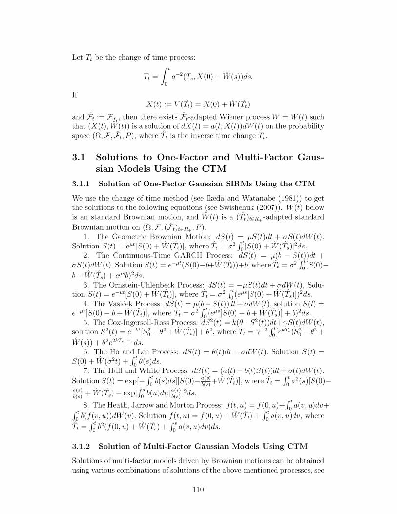
Let Tt be the change of time process:

Tt =

∫ t

0

a−2(Ts, X(0) + W (s))ds.

IfX(t) := V (Tt) = X(0) + W (Tt)

and Ft := FTt , then there exists Ft-adapted Wiener process W = W (t) suchthat (X(t),W (t)) is a solution of dX(t) = a(t,X(t))dW (t) on the probabilityspace (Ω,F , Ft, P ), where Tt is the inverse time change Tt.

3.1 Solutions to One-Factor and Multi-Factor Gaus-sian Models Using the CTM

3.1.1 Solution of One-Factor Gaussian SIRMs Using the CTM

We use the change of time method (see Ikeda and Watanabe (1981)) to getthe solutions to the following equations (see Swishchuk (2007)). W (t) belowis an standard Brownian motion, and W (t) is a (Tt)t∈R+-adapted standard

Brownian motion on (Ω,F , (Ft)t∈R+ , P ).1. The Geometric Brownian Motion: dS(t) = µS(t)dt + σS(t)dW (t).

Solution S(t) = eµt[S(0) + W (Tt)], where Tt = σ2∫ t

0[S(0) + W (Ts)]

2ds.2. The Continuous-Time GARCH Process: dS(t) = µ(b − S(t))dt +

σS(t)dW (t). Solution S(t) = e−µt(S(0)−b+W (Tt))+b, where Tt = σ2∫ t

0[S(0)−

b+ W (Ts) + eµsb)2ds.3. The Ornstein-Uhlenbeck Process: dS(t) = −µS(t)dt + σdW (t), Solu-

tion S(t) = e−µt[S(0) + W (Tt)], where Tt = σ2∫ t

0(eµs[S(0) + W (Ts)])

2ds.4. The Vasicek Process: dS(t) = µ(b−S(t))dt+σdW (t), solution S(t) =

e−µt[S(0)− b+ W (Tt)], where Tt = σ2∫ t

0(eµs[S(0)− b+ W (Ts)] + b)2ds.

5. The Cox-Ingersoll-Ross Process: dS2(t) = k(θ−S2(t))dt+γS(t)dW (t),solution S2(t) = e−kt[S2

0 − θ2 + W (Tt)] + θ2, where Tt = γ−2∫ t

0[ekTs(S2

0 − θ2 +

W (s)) + θ2e2kTs ]−1ds.6. The Ho and Lee Process: dS(t) = θ(t)dt + σdW (t). Solution S(t) =

S(0) + W (σ2t) +∫ t

0θ(s)ds.

7. The Hull and White Process: dS(t) = (a(t)− b(t)S(t))dt+σ(t)dW (t).

Solution S(t) = exp[−∫ t

0b(s)ds][S(0)−a(s)

b(s)+W (Tt)], where Tt =

∫ t0σ2(s)[S(0)−

a(s)b(s)

+ W (Ts) + exp[∫ s

0b(u)du]a(s)

b(s)]2ds.

8. The Heath, Jarrow and Morton Process: f(t, u) = f(0, u)+∫ t

0a(v, u)dv+∫ t

0b(f(v, u))dW (v). Solution f(t, u) = f(0, u) + W (Tt) +

∫ t0a(v, u)dv, where

Tt =∫ t

0b2(f(0, u) + W (Ts) +

∫ s0a(v, u)dv)ds.

3.1.2 Solution of Multi-Factor Gaussian Models Using CTM

Solutions of multi-factor models driven by Brownian motions can be obtainedusing various combinations of solutions of the above-mentioned processes, see

110

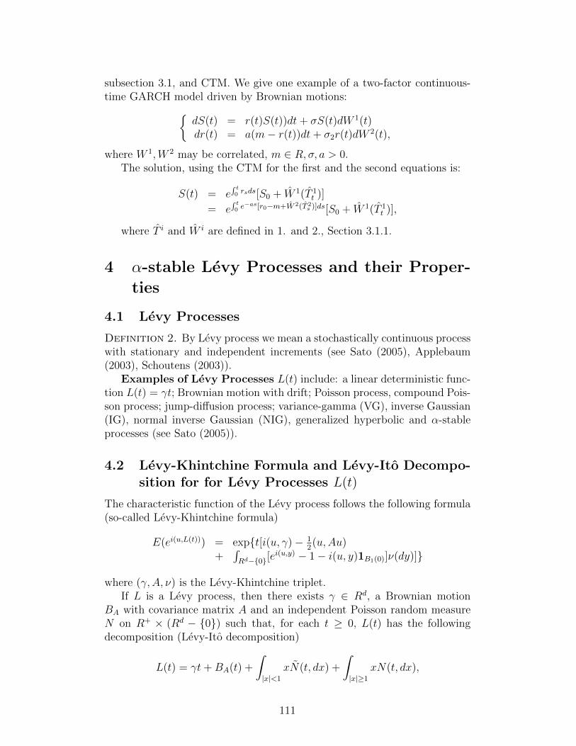
subsection 3.1, and CTM. We give one example of a two-factor continuous-time GARCH model driven by Brownian motions:

dS(t) = r(t)S(t))dt+ σS(t)dW 1(t)dr(t) = a(m− r(t))dt+ σ2r(t)dW

2(t),

where W 1,W 2 may be correlated, m ∈ R, σ, a > 0.The solution, using the CTM for the first and the second equations is:

S(t) = e∫ t0 rsds[S0 + W 1(T 1

t )]

= e∫ t0 e

−as[r0−m+W 2(T 2s )]ds[S0 + W 1(T 1

t )],

where T i and W i are defined in 1. and 2., Section 3.1.1.

4 α-stable Levy Processes and their Proper-

ties

4.1 Levy Processes

Definition 2. By Levy process we mean a stochastically continuous processwith stationary and independent increments (see Sato (2005), Applebaum(2003), Schoutens (2003)).

Examples of Levy Processes L(t) include: a linear deterministic func-tion L(t) = γt; Brownian motion with drift; Poisson process, compound Pois-son process; jump-diffusion process; variance-gamma (VG), inverse Gaussian(IG), normal inverse Gaussian (NIG), generalized hyperbolic and α-stableprocesses (see Sato (2005)).

4.2 Levy-Khintchine Formula and Levy-Ito Decompo-sition for for Levy Processes L(t)

The characteristic function of the Levy process follows the following formula(so-called Levy-Khintchine formula)

E(ei(u,L(t))) = expt[i(u, γ)− 12(u,Au)

+∫Rd−0[e

i(u,y) − 1− i(u, y)1B1(0)]ν(dy)]

where (γ,A, ν) is the Levy-Khintchine triplet.If L is a Levy process, then there exists γ ∈ Rd, a Brownian motion

BA with covariance matrix A and an independent Poisson random measureN on R+ × (Rd − 0) such that, for each t ≥ 0, L(t) has the followingdecomposition (Levy-Ito decomposition)

L(t) = γt+BA(t) +

∫|x|<1

xN(t, dx) +

∫|x|≥1

xN(t, dx),

111

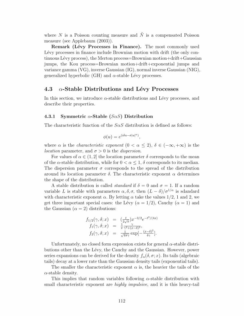
where N is a Poisson counting measure and N is a compensated Poissonmeasure (see Applebaum (2003)).

Remark (Levy Processes in Finance). The most commonly usedLevy processes in finance include Brownian motion with drift (the only con-tinuous Levy process), the Merton process=Brownian motion+drift+Gaussianjumps, the Kou process=Brownian motion+drift+exponential jumps andvariance gamma (VG), inverse Gaussian (IG), normal inverse Gaussian (NIG),generalized hyperbolic (GH) and α-stable Levy processes.

4.3 α-Stable Distributions and Levy Processes

In this section, we introduce α-stable distributions and Levy processes, anddescribe their properties.

4.3.1 Symmetric α-Stable (SαS) Distribution

The characteristic function of the SαS distribution is defined as follows:

φ(u) = e(iδu−σ|u|α),

where α is the characteristic exponent (0 < α ≤ 2), δ ∈ (−∞,+∞) is thelocation parameter, and σ > 0 is the dispersion.

For values of α ∈ (1, 2] the location parameter δ corresponds to the meanof the α-stable distribution, while for 0 < α ≤ 1, δ corresponds to its median.The dispersion parameter σ corresponds to the spread of the distributionaround its location parameter δ. The characteristic exponent α determinesthe shape of the distribution.

A stable distribution is called standard if δ = 0 and σ = 1. If a randomvariable L is stable with parameters α, δ, σ, then (L − δ)/σ1/α is sdandardwith characteristic exponent α. By letting α take the values 1/2, 1 and 2, weget three important special cases: the Levy (α = 1/2), Cauchy (α = 1) andthe Gaussian (α = 2) distributions:

f1/2(γ, δ;x) = ( t2√π)x−3/2e−t

2/(4x)

f1(γ, δ;x) = 1π

γγ2+(x−δ)2 ,

f2(γ, δ;x) = 1√4πγ

exp[− (x−δ)24γ

].

Unfortunately, no closed form expression exists for general α-stable distri-butions other than the Levy, the Cauchy and the Gaussian. However, powerseries expansions can be derived for the density fα(δ, σ;x). Its tails (algebraictails) decay at a lower rate than the Gaussian density tails (exponential tails).

The smaller the characteristic exponent α is, the heavier the tails of theα-stable density.

This implies that random variables following α-stable distribution withsmall characteristic exponent are highly impulsive, and it is this heavy-tail

112

characteristic that makes this density appropriate for modeling noise whichis impulsive in nature, for example, electricity prices or volatility.

Only moments of order less than α exist for the non-Gaussian family ofα-stable distribution. The fractional lower order moments with zero locationparameter and dispersion σ are given by

E|X|p = D(p, α)σp/α, for 0 < p < α,

D(p, α) =2pΓ( p+1

2)Γ(1− p

α)

α√πΓ(1− p

2),

where Γ(·) is the Gamma function (Sato (2005)).Since the SαS r.v. has ’infinite variance’, the covariation of two jointly

SαS real r.v. with dispersions γx and γy defined by

[X, Y ]α =E[X|Y |p−2Y ]

E[|Y |p]γy

has often been used instead of the covariance (and correlation), where γy =[Y, Y ]α is the dispersion of r.v. Y.

4.3.2 α-stable Levy Processes

Definiton 3. Let α ∈ (0, 2]. An α-stable Levy process L such thatL1 (or equivalently any Lt) has a strictly α-stable distribution (i.e., L1 ≡Sα(σ, β, δ)) for some α ∈ (0, 2] \ 1, σ ∈ R+, β ∈ [−1, 1], δ = 0 orα = 1, σ ∈ R+, β = 0, δ ∈ R). We call L a symmetric α-stableLevy process if the distribution of L1 is even symmetric α-stable (i.e.,L1 ≡ Sα(σ, 0, 0) for some α ∈ (0, 2], σ ∈ R+.) A process L is called (Tt)t∈R+-adapted if L is constant on [Tt−, Tt] for any t ∈ R+ (see Sato (2005)).

4.3.3 Properties of α-stable Levy Processes

The α-stable Levy processes are the only self-similar Levy processes such that

L(at)Law= a1/αL(t), a ≥ 0. They are either Brownian motion or pure jump.

They have characteristic exponent and Levy-Khintchine triplet known inclosed form. They also have only 4 parameters, but infinite variance (exceptfor Brownian motion). The α-stable Levy Processes are semimartingales(in this way,

∫ t0fsdLs can be defined) and α-stable Levy Processes are pure

discontinuous Markov processes with generator

Af(x) =

∫R−0

[f(x+ y)− f(x)− yf ′(y)1|y|<1(y)]Kα

|y|1+αdy.

E|L(t)|p is finite or infinite according as 0 < p < α or p > α, respectively.In particular, for an α-stable process, EL(t) = δt (1 < α < 2) (Sato (2005)).

113

5 Stochastic Differential Equations Driven by

α-Stable Levy Processes

Consider the following SDE driven by an α-stable Levy process L(t) :

dZt = b(t, Zt−)dt+ σ(t, Zt−)dL(t). (1)

Janicki et al (1996) proved that this equation has a weak solution forcontinuous coefficients a and b.

We consider below one-factor and multi-factor models described by SDEsdriven by α-stable Levy process L(t).

5.1 One-Factor α-stable Levy Models

L(t) below is a symmetric α-stable Levy process. We define below variousprocesses via SDE driven by α-stable Levy process.

1. The Geometric α-stable Levy motion: dS(t) = µS(t−)dt+σS(t−)dL(t).2. The Ornstein-Uhlenbeck Process Driven by α-stable Levy motion:

dS(t) = −µS(t−)dt+ σdL(t).3. The Vasicek Process Driven by α-stable Levy motion: dS(t) = µ(b −

S(t−))dt+ σdL(t).4. The Continuous-Time GARCH Process Driven by α-stable Levy mo-

tion: dS(t) = µ(b− S(t−))dt+ σS(t−)dL(t).5. The Cox-Ingersoll-Ross Process Driven by α-stable Levy motion:

dS(t) = k(θ − S(t−))dt+ γ√S(t−)dL(t).

6. The Ho and Lee Process Driven by α-stable Levy motion: dS(t) =θ(t−)dt+ σdL(t).

7. The Hull and White Process Driven by α-stable Levy motion: dS(t) =(a(t−)− b(t−)S(t−))dt+ σ(t)dL(t)

8. The Heath, Jarrow and Morton Process Driven by α-stable Levy mo-tion: Define the forward interest rate f(t, s), for t ≤ s, that represents theinstantaneous interest rate at time s as ‘anticipated‘ by the market at timet. The process f(t, u)0≤t≤u satisfies an equation

f(t, u) = f(0, u) +

∫ t

0

a(v, u)dv +

∫ t

0

b(f(v, u))dL(v),

where the processes a and b are continuous.We note that Eberlein & Raible (1999) considered Levy-based term struc-

ture models.

5.2 Multi-Factor α-stable Levy Models

Multi-factor models driven by α-stable Levy motions can be obtained usingvarious combinations of the above-mentioned processes. We give one exam-ple of a two-factor continuous-time GARCH model driven by α-stable Levy

114

motions.dS(t) = r(t−)S(t−))dt+ σS(t−)dL1(t)dr(t) = a(m− r(t−))dt+ σ2r(t−)dL2(t),

where L1, L2 may be correlated, m ∈ R, σi, a > 0, i = 1, 2.Also, we can consider various combinations of models, presented above,

i.e., mixed models containing Brownian and Levy motions. For example,

dS(t) = µ(b(t−)− S(t−))dt+ σS(t−)dL(t)db(t) = ξb(t)dt+ ηb(t)dW (t),

where the Brownian motion W (t) and Levy process L(t) may be correlated.

6 Change of Time Method (CTM) for SDEs

Driven by Levy Processes

We denote by Lαa.s. the family of all real measurable Ft-adapted processes a

on Ω × [0,+∞) such that for every T > 0,∫ T

0|a(t, ω)|αdt < +∞ a.s. We

consider the following SDE driven by a Levy motion:

dX(t) = a(t,X(t−))dL(t),

where L(t) is an α-stable Levy process.Theorem. (Rosinski and Woyczynski (1986), Theorem 3.1., p. 277).

Let a ∈ Lαa.s. be such that T (u) :=∫ u

0|a|αdt → +∞ a.s. as u → +∞. If

T (t) := infu : T (u) > t and Ft = FT (t), then the time-changed ctochastic

integral L(t) =∫ T (t)

0adL(t) is an Ft − α-stable Levy process, where L(t) is

Ft-adapted and Ft-α-stable Levy process. Consequently, a.s. for each t > 0∫ t0adL = L(T (t)), i.e., the stochastic integral with respect to a α-stable Levy

process is nothing but another α-stable Levy process with randomly changedtime scale.

6.1 Solutions of One-Factor Levy Models using theCTM

Below we give the solutions to the one-factor Levy models decribed by SDEsdriven by α-stable Levy process introduced in section 5.1.

Proposition 1. Let L(t) be a symmetric α-stable Levy process, and L isa (Tt)t∈R+-adapted symmetric α-stable Levy process on (Ω,F , (Ft)t∈R+ , P )).Then, we have the following solutions for the above-mentioned one-factorLevy models 1-8 (section 6.1):

1. The Geometric α-stable Levy Motion: dS(t) = µS(t−)dt+σS(t−)dL(t).Solution S(t) = eµt[S(0) + L(Tt)], where Tt = σα

∫ t0[S(0) + L(Ts)]

αds.2. The Ornstein-Uhlenbeck Process Driven by α-stable Levy Motion:

dS(t) = −µS(t−)dt+ σdL(t). Solution S(t) = e−µt[S(0) + L(Tt)], whereTt = σα

∫ t0(eµs[S(0) + L(Ts)])

αds.

115

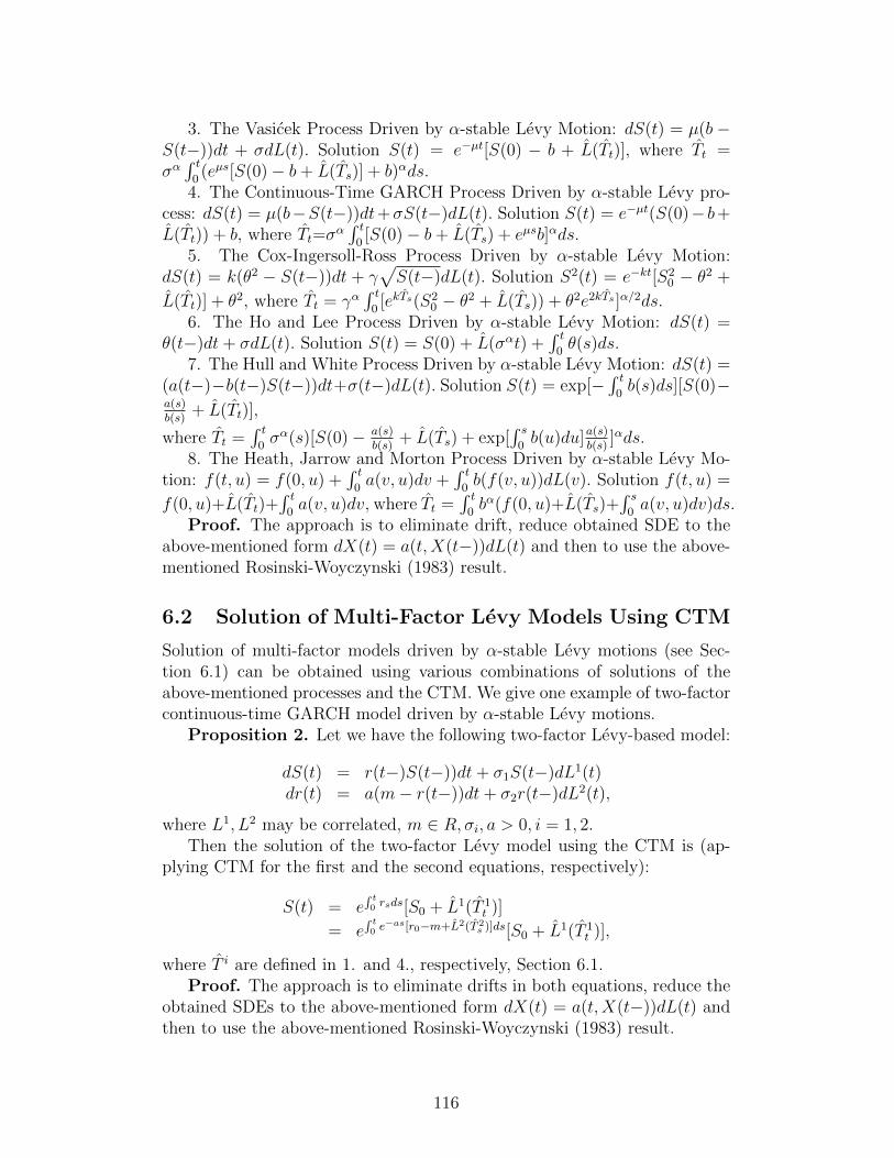
3. The Vasicek Process Driven by α-stable Levy Motion: dS(t) = µ(b−S(t−))dt + σdL(t). Solution S(t) = e−µt[S(0) − b + L(Tt)], where Tt =σα∫ t

0(eµs[S(0)− b+ L(Ts)] + b)αds.

4. The Continuous-Time GARCH Process Driven by α-stable Levy pro-cess: dS(t) = µ(b−S(t−))dt+σS(t−)dL(t). Solution S(t) = e−µt(S(0)− b+L(Tt)) + b, where Tt=σ

α∫ t

0[S(0)− b+ L(Ts) + eµsb]αds.

5. The Cox-Ingersoll-Ross Process Driven by α-stable Levy Motion:dS(t) = k(θ2 − S(t−))dt + γ

√S(t−)dL(t). Solution S2(t) = e−kt[S2

0 − θ2 +

L(Tt)] + θ2, where Tt = γα∫ t

0[ekTs(S2

0 − θ2 + L(Ts)) + θ2e2kTs ]α/2ds.6. The Ho and Lee Process Driven by α-stable Levy Motion: dS(t) =

θ(t−)dt+ σdL(t). Solution S(t) = S(0) + L(σαt) +∫ t

0θ(s)ds.

7. The Hull and White Process Driven by α-stable Levy Motion: dS(t) =(a(t−)−b(t−)S(t−))dt+σ(t−)dL(t). Solution S(t) = exp[−

∫ t0b(s)ds][S(0)−

a(s)b(s)

+ L(Tt)],

where Tt =∫ t

0σα(s)[S(0)− a(s)

b(s)+ L(Ts) + exp[

∫ s0b(u)du]a(s)

b(s)]αds.

8. The Heath, Jarrow and Morton Process Driven by α-stable Levy Mo-tion: f(t, u) = f(0, u) +

∫ t0a(v, u)dv +

∫ t0b(f(v, u))dL(v). Solution f(t, u) =

f(0, u)+L(Tt)+∫ t

0a(v, u)dv, where Tt =

∫ t0bα(f(0, u)+L(Ts)+

∫ s0a(v, u)dv)ds.

Proof. The approach is to eliminate drift, reduce obtained SDE to theabove-mentioned form dX(t) = a(t,X(t−))dL(t) and then to use the above-mentioned Rosinski-Woyczynski (1983) result.

6.2 Solution of Multi-Factor Levy Models Using CTM

Solution of multi-factor models driven by α-stable Levy motions (see Sec-tion 6.1) can be obtained using various combinations of solutions of theabove-mentioned processes and the CTM. We give one example of two-factorcontinuous-time GARCH model driven by α-stable Levy motions.

Proposition 2. Let we have the following two-factor Levy-based model:

dS(t) = r(t−)S(t−))dt+ σ1S(t−)dL1(t)dr(t) = a(m− r(t−))dt+ σ2r(t−)dL2(t),

where L1, L2 may be correlated, m ∈ R, σi, a > 0, i = 1, 2.Then the solution of the two-factor Levy model using the CTM is (ap-

plying CTM for the first and the second equations, respectively):

S(t) = e∫ t0 rsds[S0 + L1(T 1

t )]

= e∫ t0 e

−as[r0−m+L2(T 2s )]ds[S0 + L1(T 1

t )],

where T i are defined in 1. and 4., respectively, Section 6.1.Proof. The approach is to eliminate drifts in both equations, reduce the

obtained SDEs to the above-mentioned form dX(t) = a(t,X(t−))dL(t) andthen to use the above-mentioned Rosinski-Woyczynski (1983) result.

116

Important Remark. Kallsen & Shiryaev (2002) showed that the Rosinski& Woyczynski (1986) statement cannot be extended to any other Levy pro-cess but α-stable processes. If one considers only nonnegative integrands a indX(t) = a(t,X(t−))dL(t), then we can extend their statement to asymmetricα-stable Levy processes.

7 Applications in Financial and Energy Mar-

kets

In this section, we consider various applications of the change of time methodfor Levy-based SDEs arising in financial and energy markets: swap and op-tion pricing, interest derivatives pricing and forward and futures contractspricing.

7.1 Variance Swaps for Levy-Based Heston Model

Assume that in the risk-neutral world the underlying asset St and the vari-ance follow the following model:

dStSt

= rtdt+ σtdwtdσ2

t = k(θ2 − σ2t )dt+ γσtdLt,

where rt is the deterministic interest rate, σ0 and θ are the short and longvolatilities, k > 0 is a reversion speed, γ > 0 is a volatility (of volatility)parameter, wt and Lt are independent standard Wiener and α-stable Levyprocesses (α ∈ (0, 2]).

The solution for the second equation has the following form:

σ2(t) = e−kt[σ20 − θ2 + L(Tt)] + θ2,

where Tt = γα∫ t

0[ekTs(σ2

0 − θ2 + L(Ts)) + θ2e2kTs ]α/2ds.A variance swap is a forward contract on annualized variance, the square

of the realized volatility. Its payoff at expiration is equal to

N(σ2R(S)−Kvar),

where σ2R(S) is the realized stock variance (quoted in annual terms) over the

life of the contract,

σ2R(S) :=

1

T

∫ T

0

σ2(s)ds,

Kvar is the delivery price for variance, and N is the notional amount.Valuing a variance forward contract or swap is no different from valuing

any other derivative security. The value of a forward contract P on future

117

realized variance with strike price Kvar is the expected present value of thefuture payoff in the risk-neutral world:

Pvar = Ee−rT (σ2R(S)−Kvar),

where r is the risk-free discount rate corresponding to the expiration date T,and E denotes the expectation.

The realized variance in our case is:

σ2R(S) :=

1

T

∫ T

0

σ2(s)ds =1

T

∫ T

0

e−ks[σ20 − θ2 + L(Ts)] + θ2ds.

The value of the variance swap then is:

Pvar = Ee−rT (σ2R(S)−Kvar)

= Ee−rT ( 1T

∫ T0e−ks[σ2

0 − θ2 + L(Ts)] + θ2ds−Kvar).

Thus, for calculating variance swaps we need to know only Eσ2R(S),

namely, the mean value of the underlying variance, or EL(Ts).Only moments of order less than α exist for the non-Gaussian family of

α-stable distributions. We suppose that 1 < α < 2 to find EL(Ts).The value of a variance swap for the Levy-based Heston model is:

Pvar = e−rT [1− e−kT

kT(σ2

0 − θ2) + θ2 +δT

2−Kvar],

where δ is a location parameter.If δ = 0, then the value of a variance swap for the Levy-based Heston

model is:

Pvar = e−rT [1− e−kT

kT(σ2

0 − θ2) + θ2 −Kvar],

which coincides with the well-known result by Brockhaus and Long (2000)and Swishchuk (2004).

7.2 Volatility Swaps for Levy-Based Heston Model?

A stock volatility swap is a forward contract on the annualized volatility. Itspayoff at expiration is equal to

N(σR(S)−Kvol),

where σR(S) is the realized stock volatility (quoted in annual terms) over thelife of contract,

σR(S) :=

√1

T

∫ T

0

σ2sds,

118

σt is a stochastic stock volatility, Kvol is the annualized volatility deliveryprice, and N is the notional amount

To calculate volatility swaps we need more. From Brockhaus-Long(2000) approximation (which used the second order Taylor expansion forthe function

√x) we have:

E√σ2R(S) ≈

√EV − V arV

8EV 3/2,

where V := σ2R(S) and V arV

8EV 3/2 is the convexity adjustment.

Thus, to calculate the value of volatility swaps

Pvol = e−rT (EσR(S) −Kvol)

we need both EV and V arV .For SαS processes only the moments of order p < α exist, α ∈ (0, 2].Since the SαS r.v. has ’infinite variance’, the covariation of two jointly

SαS real r.v. with dispersions γx and γy defined by

[X, Y ]α =E[X|Y |p−2Y ]

E[|Y |p]γy,

where γy = [Y, Y ]α is the dispersion of r.v. Y, has often been used instead ofthe covariance (and correlation).

One of possible ways to get volatility swaps for the Levy-based Hestonmodel is to use covariation.

7.3 Gaussian- and Levy-based SABR/LIBOR MarketModels

SABR model (see Hagan, Kumar, Lesniewski and Woodward (2002)) andthe Libor Market Model (LMM) (Brace, Gatarek and Musiela (BGM, 1996),Piterbarg (2003)) have become industry standards for pricing plain-vanillaand complex interest rate products, respectively.

The Gaussian-based SABR model (Hagan, Kumar, Lesniewski and Wood-ward (2002)) is a stochastic volatility model in which the forward value sat-isfies the following SDE:

dFt = σtFβt dW

1t

dσt = νσtdW2t .

In a similar way, we introduce the Levy-based SABR model, a stochasticvolatility model in which the forward value satisfies the following SDE:

dFt = σtFβt dWt

dσt = νσtdLt,

where L(t) is an α-stable Levy process.

119

The solution of Levy-based SABR model using a change of time methodhas the following expression:

Ft = F0 + W (T 1t ),

T 1t =

∫ t

0

σ−2T 1s

(F0 + W (s))−2βds,

σt = σ0 + L(T 2t ),

T 2t = ν−α

∫ t

0

(σ0 + L(s))−αds.

The expressions for Ft and σt give the possibility to calculate many financialderivatives.

7.4 Energy Forwards and Futures

Random variables following α-stable distribution with small characteristicexponent are highly impulsive, and it is this heavy-tail characteristic thatmakes this density appropriate for modeling noise which is impulsive in na-ture, for example, energy prices such as electricity. Here, we introduce twoLevy-based models in energy market: two-factor Levy-based Schwartz-Smithand three-factor Schwartz models. We show how solve them using the changeof time method.

7.4.1 Levy-based Schwartz-Smith Model

We introduce the Levy-based Schwartz-Smith model:ln(St) = κt + ξtdκt = (−kκt − λκ)dt+ σκdLκdξt = (µξ − λξ)dt+ σξdWξ,

where St is the current spot price, κt is the short-term deviation in prices,and ξt is the equilibrium price level.

Let Ft,T denote the market price for a futures contract with maturity T,then:

ln(Ft,T ) = e−k(T−t)κt + ξt + A(T − t),where A(T − t) is a deterministic function with explicit expression. We notethat κt, using change of time for α-stable processes, can be presented in thefollowing form:

κt = e−kt[κ0 +λκk

+ Lκ(Tt)],

Tt = σακ

∫ t

0

(e−ks[κ0 +λκk

+ Lκ(Ts)]−λκk

)αds.

In this way, the market price for a futures contract with maturity T hasthe following form:

120

ln(Ft,T ) = e−kT [κ0 + λκk

+ Lκ(Tt)]+ ξ0 + (µξ − λξ)t+ σξWξ + A(T − t),

where the Levy process Lκ and Wiener process Wξ may be correlated.If α ∈ (1, 2], then we can calculate the value of Levy-based futures con-

tracts.

7.4.2 Levy-based Schwartz Model

We also introduce a Levy-Based Schwartz model:d ln(St) = (rt − δt)Stdt+ Stσ1dW1

dδt = k(a− δt)dt+ σ2dLdrt = a(m− rt)dt+ σ3dW2,

where the Wiener processes W1,W2 and α-stable Levy process L may becorrelated. δt and rt are the instantaneous convenience yield and interestrate, respectively.

We note that:

δt = ekt(δ0 − a+ L(Tt)),

Tt = σα2∫ t

0(eks[δ0 − a+ L(Ts)] + a)αds

andrt = eat(r0 −m+ W2(Tt)),

Tt = σ23

∫ t0(eas[r0 −m+ W2(Ts)] +m)2ds.

The solution for ln[St] :

ln[St] = e∫ t0 [eas(r0−m+W2(T 2

s ))−eks(δ0−a+L(Ts))]ds[lnS0 + W1(T 1t )].

In this way, the futures contract has the following form:

ln(Ft,T ) = 1−e−k(T−t)

kδt + 1−e−a(T−t)

art + ln(St) + C(T − t)

= 1−e−k(T−t)

k[ekt(δ0 − a+ L(Tt))]

+ 1−e−a(T−t)

aeat(r0 −m+ W2(T 2

t ))

+ exp∫ t

0(eas(r0 −m+ W2(T 2

s ))

− eks(δ0 − a+ L(Ts)))ds[ln(S0) + W1(T 1t )]

+ C(T − t),

where C(T − t) is a deterministic explicit function. If α > 1, then we cancalculate the value of a futures contract.

121

References

Andersen, L. and Andersen, J. Volatility skews and extensions of theLibor Market Model. Applied Mathematical Finance, 7:1-32, March 2000.

Andersen, L. and Andersen, J. Volatile volatilites. Risk, 15(12), Decem-ber 2002.

Applebaum, D. Levy Processes and Stochastic Calculus, Cambridge Uni-versity Press, 2003.

Barndorff-Nielsen, E. and Shiryaev, A.N. Change of Time and Change ofMeasures, World Scientific, 2010, 305 p. (to appear)

Barndorff-Nielsen, O.E., Nicolato, E. and Shephard, N. Some recent de-velopment in stochastic volatility modeling, Quantitative Finance, 2, 11-23,1966.

Bates, D. Jumps and stochastic volatility: the exchange rate processesimplicit in Deutschemark options, Review Finance Studies, 9, pp. 69-107,1996.

Benth, F., Benth, J. and Koekebakker, S. Stochastic Modelling of Elec-tricity and Related Markets, World Sci., 2008.

Bingham, N. and Kiesel, B. Risk-Neutral Valuations, Pricing and Hedgingof Financial Derivatives, Springer Finance, London, 1998.

Bjork, T. and Landen, C. On the term structure of futures and forwardprices. In: Geman, H.,Madan, D., Pliska, S. and Vorst, T., Editors. Mathe-matical Finance-Bachelier Congress 2000, Springer, Berlin (2002), pp. 111-149.

Black, F. The pricing of commodity contracts, J. Financial Economics,3, 167-179, 1976.

Bochner, S. Diffusion equation and stochastic processes. Proc. Nat.Acad. Sci. USA, 85, 369-370, 1949.

Brace, A., Gatarek, D. and Musiela, M. The market model of interestrate dynamics, Math. Finance, 1997, 4, 127-155.

Brigo, D. and Mercurio, F. Interest-Rate Models-Theory and Practice.Springer Verlag, 2001.

Brockhaus, O. and Long, D. Volatility swaps made simple, RISK, Jan-uary, 92-96, 2000.

Carmona, R. and Ludkovski, M. Spot convenience yield models for theenergy markets, working paper, Princeton University, 2003.

Carr, P., Geman, H., Madan, D. and Yor, M. Stochastic volatility for Levyprocesses.// Mathematical Finance, vol. 13, No. 3 (July 2003), 345-382.

Carr, P. and Madan, D. Option valuation using the fast Fourier transform.Journal of Computational Finance, 2:61-73, 1999.

Carr, P. and Wu, L. The finite moment logstable process and optionpricing. The Journal of Finance, LVIII(2):753-777,April 2003.

Carr, P. and Wu, L. Time-changed Levy processes and option pricing.Journal of Financial Economics, 71 (2004) 113-141.

122

Cartea, A. and Howison, S. Option pricing with Levy-stable processesgenerated by Levy-stable integrated variance. Birkbeck Working Papers inEconomics & Finance, Birkbeck, University of London, February 24 2006.

Chernov, R., Gallant, E., Ghysels, E. and Tauchen, G. Alternative modelsfor stock price dynamics, Journal of Econometrics, 116, pp. 225-257, 2003.

Cherny, A. and Shiryaev, A. Change of time and measure for Levy pro-cesses. Lectures for Summer School ’From Levy Processes to Semimartingales-Recent Theoretical Developments and Applications to Finance’, Aarhus, Au-gust 2002.

Clark, P. A subordinated stochastic process model with fixed variance forspeculative prices, Econometrica, 41, 135-156, 1973.

Cont, R. and Tankov, P. Financial Modeling with Jump Processes, Chap-man & Hall/CRC Fin. Math. Series, 2004.

Cox, J., Ingersoll, J. and Ross, S. A theory of the term structure of interestrate. Econometrics, 53 (1985), pp. 385-407.

Dambis, K.E. On the decomposition of continuous submartingales, The-ory Probabability and its Appl., 10, 4091-410, 1965.

Dubins and Schwartz. On continuous martingales, Proc. Nat. Acad.Sciences, USA, 53, 913-916, 1965.

Demeterfi, K., Derman, E., Kamal, M. and Zou, J. A guide to volatilityand variance swaps, The Journal of Derivatives, Summer, 9-32, 1999.

Eberlein, E., Kallsen, J. and Kirsten, J. Risk management based onstochastic volatility. Preprint 72, University of Freiburg, 2001.

Eydeland, E. and Geman, H. Pricing power derivatives, RISK, Septem-ber, 1998.

Elliott, R. and Swishchuk, A. Pricing options and variance swaps inMarkov-modulated Brownian markets, In: Hidden Markov Models in Fi-nance, Springer, 2007, ed. R. Mamon and R. Elliott.

Feller, W. Introduction to Probability Theory and its Applications, v. II,Wiley & Sons, 1966.

Fouque, J.-P., Papanicolaou, G. and Sircar, K. R. Derivatives in FinancialMarkets with Stochastic Volatilities. Springer-Verlag, 2000.

Fouque, J.-P. and Han, C.-H. A control variate method to evaluate optionprices under multi-factor stochastic volatility models, working paper, 2003.

Geman, H. Commodities and Commodity Derivatives: Modelling andPricing for Agricaltural, Metals and Energy, Wiley, 2005.

Geman, H., Madan, D. and Yor, M. Time changes for Levy processes,Math. Finance, 11, 79-96.

Geman, H. and Roncoroni, R. Understanding the fine structure of elec-tricity prices, Journal of Business, 2005.

Geman, H. Scarcity and price volatility in oil markets (EDF Trading Tech-nical Report), 2000.

Geman, H. Commodity and Commodity Derivatives: Modelling and Pric-ing for Agriculturals, Metals and Energy. Wiley/Finance, 2005.

123

Gibson and Schwartz, E. Stochastic convenience yield and the pricing ofoil contigent claims, Journal of Finance, 45, 959–976, 1990.

Gerber, H. U. and Shiu, E. S. W. Option pricing by Esscher-transforms.Transactions of the Society of Actuaries, 46, 99-191, 1994.

Girsanov, I. On transforming a certain class of stochastic processes by ab-solutely continuous subtitution of measures. Theory Probab. Appl., 5(1960),3, pp. 285-301.

Glasserman, P. and Kou, S. The term structure of simple forwad rateswith jumps risk. Columbia working paper, 1999.

Glasserman, P. and N. Merener. Numerical solution of jump diffusionLIBOR market models, Fin. Stochastics, 2003, 7, 1-27.

Hagan, P., Kumar, D. and Lesniewski, A. Managing smile risk. WilmottMagazine, autumn, 2002, p. 84-108.

Hearth, D., Jarrow, R. and Morton, A. Bond pricing and the term struc-ture of the interest rates: A new mathodology. Econometrica, 60, 1 (1992),pp. 77-105.

Henry-Labordere, P. Combining the SABR and LMM models. Risk, Oc-tober, 2007, p. 102-107.

Heston, S. A closed-form solution for options with stochastic volatilitywith applications to bond and currency options, Review of Financial Studies,6, 327-343, 1993.

Ho, T. and Lee, S. Term structure movements and pricing interest ratecontigent claim. J. of Finance, 41 (December 1986), pp. 1011-1029.

Hoffman-Jorgensen, J. Sum of independent Banach space valued randomvariables, Studia Matematika, Warszawa, 1, 52, 1974, pp. 159-186.

Hull, J. and White, A. Pricing interest rate derivative securities. Reviewof Fin. Studies, 3,4 (1990), pp. 573-592.

Huff, B. The loose subordination of differential processes to Brownianmotion, Ann. Math. Statist., 40, 1603-1609.

Ikeda, N. Watanabe, S. Stochastic Differential Equations and DiffusionProcesses. North-Holland/Kodansha Ltd., Tokyo, 1981.

Jacod, J. Calcul Stochastique et Problemes de Martingales, Lecture Notesin Mathematics 714, Springer-Verlag, 1979.

Jacod, J. and Shiryaev, A. Limit Theorems for Stochastic Processes.Springer-Verlag, 1987.

Jamshidian, F. LIBOR and swap market models and measures, Fin.Stochastics, 1 (4), 293-330, 1997.

Javaheri, A., Wilmott, P. and Haug, E. GARCH and volatility swaps,Wilmott Technical Article, January, 17p., 2002.

Johnson, H. Option pricing when the variance rate is changing. Workingpaper, University of california, Los Angeles, 1979.

Johnson, H. and Shanno, D. Option pricing when the variance is changing,J. Financial Quant. Anal., 22, 143-152.

Joshi, M. and Rebonato, R. A displaced-diffusion stochastic volatility Li-bor market model: motivation, definition and implementation. Qunatitative

124

Finance, 3, 2003, p. 458-469.Kallenberg, O. Some time change representations of stable integrals, via

predictable transformations of local martingales. Stochastic Processes andTheir Applications, 40 (1992), 199-223.

Kallsen, J. and Shiryaev, A. Time change representation of stochasticintegrals, Theory Probab. Appl., vol. 46, N. 3, 522-528, 2002.

Knight, F. A reduction of continuous, square-integrable martingales toBrownian motion, in: H. Dinges, ed., Martingales, Lecture Notes in Math.No. 190 (Springer, Berlin, 1971) pp. 19-31.

Levy, P. Processus Stochastiques et Mouvement Brownian, 2nd ed., Gauthier-Villars, Paris, 1965.

Madan, D. and Seneta, E. The variance gamma (VG) model for sharemarket returns, J. Business 63, 511-524.

Meyer, P. A. Demonstration simplifiee d’un theoreme de Knight, in: Sem-inaire de Probabilites V, Lecture Notes in Math. No. 191 (Springer, Berlin,1971) pp. 191-195.

Molina, G., Han, C.-H. and Fouque, J.-P. MCMC Estimation of Multi-scale Stochastic Volatility Models, Preprint, 2003.

Monroe, I. On embedding right continuous martingales in Brownian mo-tion, Ann. Math. Statist., 43, 1293-1311, 1972.

Monroe, I. Processes that can be embedded in Brownian motion, TheAnnals of Probab., 6, No. 1, 42-56, 1978.

Ornstein, L. and G.Uhlenbeck. On the theory of Brownian motion. Phys-ical Review, 36 (1930), 823-841.

Papangelou, F. Integrability of expected increments of point processesand a related random change of scale, Trans. Amer. Math. Soc. 165 (1972)486-506.

Pilipovic, D. Valuing and Managing Energy Derivatives, New York, McGraw-Hill, 1997.

Piterbarg, V. Astochastic volatility forward Libor model with a termstructure of volatility smiles. October, 2003(http://ssrn.com/abstract=472061)

Piterbarg, V. Time to smile. Risk, May 2005, p. 87-92.Protter, P. Stochastic Integration and Differential Equations, Springer,

2005.Raible, S. Levy processes in finance: theory, numerics, and empirical

facts. PhD thesis, Freiburg, 2000.Rebonato, R. A time-homogeneous, SABR-consistent extension of the

LMM, Risk, 2007.Rebonato, R. Modern pricing of interest rate derivatives: the Libor mar-

ket model and beyond. Princton University Press, 2002.Rebonato, R. and Joshi, M. A joint empirical and theoretical investi-

gation of the models of deformation of swaption matrices: implications forthe stochastic-volatility Libor market model. Intern. J. Theoret. AppliedFinance, 5(7), 2002, p. 667-694.

125

Rebonato, R. and Kainth, D. A two-regime, stochastic-volatility exten-sion of the Libot market model. Intern. J. Theoret. Applied Finance, 7(5),2004, p. 555-575.

Rendleman, R. and Barttler, B. The pricing of options on debt securities,Journal of Financial and Quantitative Analysis, 15 (March 1980), 11-24.

Rosinski, J. and Woyczinski, W. On Ito stochastic integration with re-spect to p-stable motion: Inner clock, intagrability of sample paths, doubleand multiple integrals, Ann. Probab., 14 (1986), 271-286

Samorodnitsky, G. and Taqqu, M. Stable Non-Gaussian Random Pro-cesses: Stochastic Models with Infinite Variance. Chapman and Hall, NewYork, 1994.

Sato, K. Levy Processes and Infinitely Divisible Distributions. CambridgeUniversity Press, Cambridge, UK, 1999.

Schoutens, W. Levy Processes in Finance. Pricing Financial Derivatives.Wiley & Sons, 2003.

Schwartz, E. The stochastic behaviour of commodity prices: implicationsfor pricing and hedging, J. Finance, 52, 923-97, 1997.

Sin, C. Alternative interest rate volatility smile models. Risk conferenceproceedings, 2002.

Schwartz, E. Short-Term Variations and Long-Term Dynamics in Com-modity Prices, Management Science, Volume 46, Issue 7, 1990.

Schwartz, E. The stochastic behaviour of commodity prices: implicationsfor pricing and hedging, J. Finance, 52, 923–973, 1997.

Shiryaev, A. Essentials of Stochastic Finance, World Scientific, 2008.Skorokhod, A. Random Processes with Independent Increments, Nauka,

Moscow, 1964. (English translation: Kluwer AP, 1991).Skorokhod, A. Studies in the Theory of Random Processes, Addison-

Wesley, Reading, 1965.Swishchuk, A. Levy-based interest rate derivatives: change of time and

PIDEs, submitted to CAMQ, June 10, 2008(available at http://papers.ssrn.com/sol3/papers.cfm?abstract id=1322532).

Swishchuk, A. Multi-factor Levy models: change of time and pricing offinancial and energy derivatives, December 3, 2008(available at http://papers.ssrn.com/sol3/papers.cfm?abstract id=1322534).

Swishchuk, A. Multi-factor Levy models for pricing of financial and energyderivatives, CAMQ, V. 17, No. 4, Winter, 2009

Swishchuk, A. Modelling and valuing of variance and volatility swaps forfinancial markets with stochastic volatilites, Wilmott Magazine, TechnicalArticle, N0. 2, September, 2004, 64-72.

Swishchuk, A. Modeling and Pricing of Variance Swaps for StochasticVolatilities with Delay, WILMOTT Magazine, Issue 19, September 2005, pp.63-73.

Swishchuk, A. Modeling and Pricing of Variance Swaps for Multi-FactorStochastic Volatilities with Delay, Canad. Appl. Math. Quart., Volume 14,Number 4, Winter 2006.

126

Swishchuk, A. Change of time method in mathematical finance, Canad.Appl. Math. Quart., vol. 15, No. 3, 2007, p. 299-336.

Swishchuk, A. Explicit option pricing formula for a mean-reverting assetin energy market, J. of Numer. Appl. Math., Vol. 1(96), 2008, pp. 216-233.

Swishchuk, A. Pricing of variance and volatility swaps with semi-Markovvolatilities, CAMQ, 2010 (to appear).

Theoret, R., Zabre, L. and Rostan, P. (2002): Pricing volatility swaps:empirical testing with Canadian data. Working paper, Centre de Rechercheen Gestion, Document 17-2002, July 2002.

Vasicek, O. An equilibrium characterization of the term structure. J. ofFinan. Economics, 5 (1977), pp. 177-188.

Villaplana A two-state variables model for electricity prices, Third WorldCongress of the Bachelier Finance Society, Chicago, 2004.

Wilmott, P. Paul Wilmott on Quantitative Finance, New York, Wiley,2000.

127

Chapter 8: CTM and Variance and Volatility

Swaps in Energy Markets

’Energy and persistence conquer all things,’-Benjamin Franklin.

1 Introduction

This Chapter is devoted to the pricing of variance and volatility swaps inenergy market. We found explicit variance swap formula and closed formvolatility swap formula (using change of time) for energy asset with stochasticvolatility that follows continuous-time mean-reverting GARCH (1,1) model.Numerical example is presented for AECO Natural Gas Index (1 May 1998-30April 1999).

Variance swaps are quite common in commodity, e.g., in energy mar-ket, and they are commonly traded. We consider Ornstein-Uhlenbeck pro-cess for commodity asset with stochastic volatility following continuous-timeGARCH model or Pilipovic (1998) one-factor model. The classical stochasticprocess for the spot dynamics of commodity prices is given by the Schwartz’model (1997). It is defined as the exponential of an Ornstein-Uhlenbeck(OU) process, and has become the standard model for energy prices possess-ing mean-reverting features.

In this paper, we consider a risky asset in energy market with stochasticvolatility following a mean-reverting stochastic process satisfying the follow-ing SDE (continuous-time GARCH(1,1) model):

dσ2(t) = a(L− σ2(t))dt+ γσ2(t)dWt,

where a is a speed of mean reversion, L is the mean reverting level (orequilibrium level), γ is the volatility of volatility σ(t), Wt is a standard Wienerprocess. Using a change of time method we find an explicit solution of thisequation and using this solution we are able to find the variance and volatilityswaps pricing formula under the physical measure. Then, using the sameargument, we find the option pricing formula under risk-neutral measure. Weapplied Brockhaus-Long (2000) approximation to find the value of volatil;ityswap. A numerical example for the AECO Natural Gas Index for the period1 May 1998 to 30 April 1999 is presented.

Commodities are emerging as an asset class in their own. The rangeof products offered to investors range from exchange traded funds (ETFs)to sophisticated products including principal protected structured notes onindividual commodities or baskets of commodities and commodity range-accrual or varinace swap.

More and more institutional investors are including commodities in theirasset allocation mix and hedge funds are also increasingly active playersin commodities. Example: Amaranth Advisors lost USD 6 billion during

128

September 2006 from trading natural gas futures contracts, leading to thefund’s demise.

Concurrent with these developments, a number of recent papers haveexamined the risk and return characteristics of investments in individualcommodity futures or commodity indices composed of baskets of commodityfutures. See, e.g., Erb and Harvey (2006), Gorton and Rouwenhorst (2006),Ibbotson (2006), Kan and Oomen (2007).

However, since all but the most plain-vanilla investments contain an ex-posure to volatility, it is equally important for investors to understand therisk and return characteristics of commodity volatilities.

Our focus on energy commodities derives from two resons:1) energy is the most important commodity sector, and crude oil and

natural gas constitute the largest components of the two most widely trackedcommodity indices: the Standard & Poors Goldman Sachs Commodity Index(S&P GSCI) and the Dow Jones-AIG Commodity Index (DJ-AIGCI).

2) existence of a liquid options market: crude oil and natural gas indeedhave the deepest and most liquid options marketss among all commodities.

The idea is to use variance (or volatility) swaps on futures contracts.At maturity, a variance swap pays off the difference between the realized

variance of the futures contract over the life of the swap and the fixed varianceswap rate.

And since a variance swap has zero net market value at initiation, absenceof arbitrage implies that the fixed variance swap rate equals to conditionalrisk-neutral expectation of the realized variance over the life of swap.

Therefore, e.g., the time-series average of the payoff and/or excess returnon a variance swap is a measure of the variance risk premium.

Variance risk premia in energy commodities, crude oil and natural gas,has been considered by A. Trolle and E. Schwartz (2009).

The same methodology as in Trolle & Schwartz (2009) was used by Carr& Wu (2009) in their study of equity variance risk premia. The idea was touse variance swaps on futures contracts.

The study in Trolle&Schwartz (2009) is based on daily data from January2, 1996 until November 30, 2006-a total of 2750 business days. The sourceof the data is NYMEX.

Trolle & Schwartz (2009) found that:1) the average variance risk premia are negative for both energy commodi-

ties but more strongly statistically significant for crude oil than for naturalgas;

2) the natural gas variance risk premium (defined in dollars terms or inreturn terms) is higher during the cold months of the year (seasonality andpeaks for natural gas variance during the cold months of the year);

3) energy risk premia in dollar terms are time-varying and correlatedwith the level of the variance swap rate. In contrast, energy variance riskpremia in return terms, paerticularly in the case of natural gas, are muchless correlated with the varinace swap rate.

129

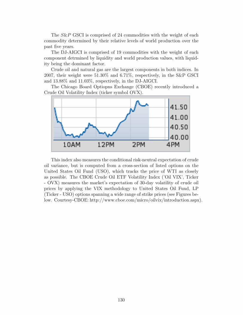
The S&P GSCI is comprised of 24 commodities with the weight of eachcommodity determined by their relative levels of world production over thepast five years.

The DJ-AIGCI is comprised of 19 commodities with the weight of eachcomponent detrmined by liquidity and world production values, with liquid-ity being the dominant factor.

Crude oil and natural gas are the largest components in both indices. In2007, their weight were 51.30% and 6.71%, respectively, in the S&P GSCIand 13.88% and 11.03%, respectively, in the DJ-AIGCI.

The Chicago Board Optiopns Exchange (CBOE) recently introduced aCrude Oil Volatility Index (ticker symbol OVX).

This index also measures the conditional risk-neutral expectation of crudeoil variance, but is computed from a cross-section of listed options on theUnited States Oil Fund (USO), which tracks the price of WTI as closelyas possible. The CBOE Crude Oil ETF Volatility Index (’Oil VIX’, Ticker- OVX) measures the market’s expectation of 30-day volatility of crude oilprices by applying the VIX methodology to United States Oil Fund, LP(Ticker - USO) options spanning a wide range of strike prices (see Figures be-low. Courtesy-CBOE: http://www.cboe.com/micro/oilvix/introduction.aspx).

130

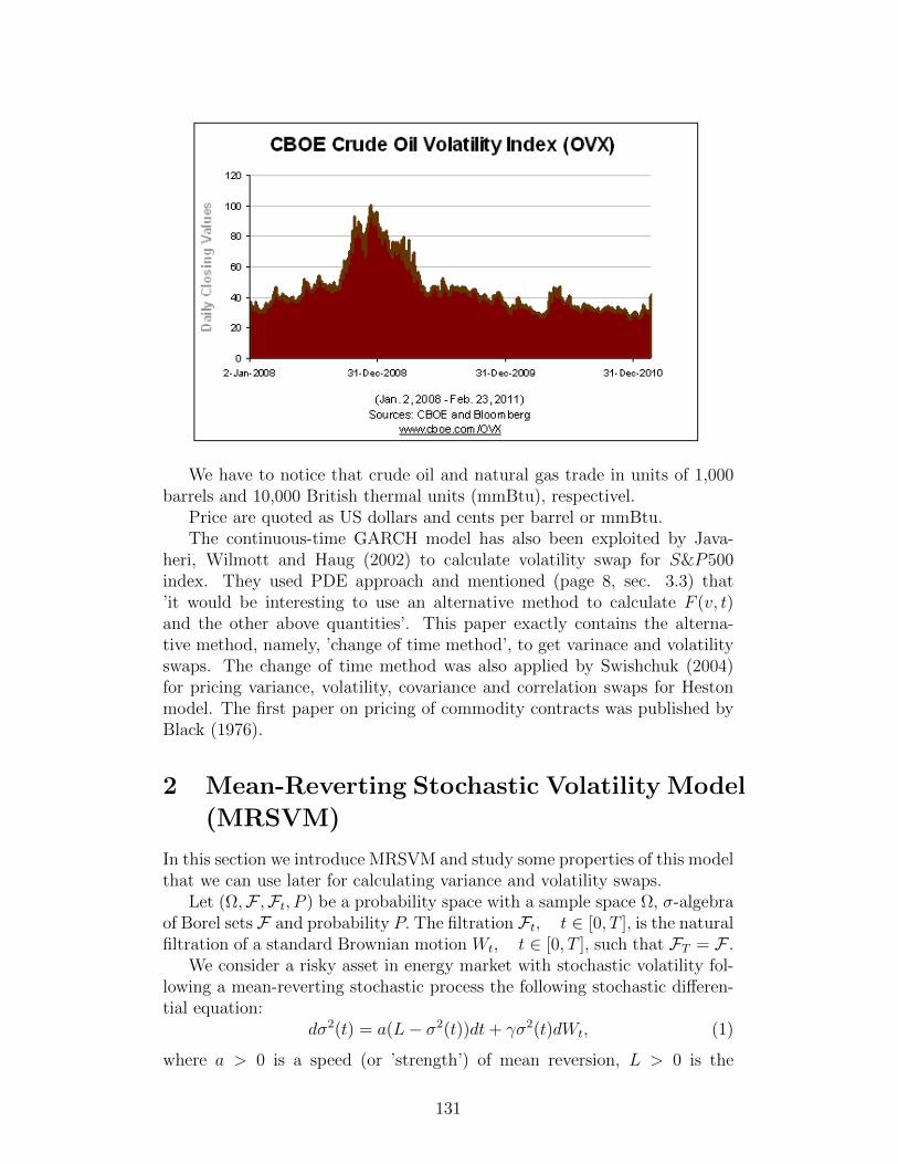
We have to notice that crude oil and natural gas trade in units of 1,000barrels and 10,000 British thermal units (mmBtu), respectivel.

Price are quoted as US dollars and cents per barrel or mmBtu.The continuous-time GARCH model has also been exploited by Java-

heri, Wilmott and Haug (2002) to calculate volatility swap for S&P500index. They used PDE approach and mentioned (page 8, sec. 3.3) that’it would be interesting to use an alternative method to calculate F (v, t)and the other above quantities’. This paper exactly contains the alterna-tive method, namely, ’change of time method’, to get varinace and volatilityswaps. The change of time method was also applied by Swishchuk (2004)for pricing variance, volatility, covariance and correlation swaps for Hestonmodel. The first paper on pricing of commodity contracts was published byBlack (1976).

2 Mean-Reverting Stochastic Volatility Model

(MRSVM)

In this section we introduce MRSVM and study some properties of this modelthat we can use later for calculating variance and volatility swaps.

Let (Ω,F ,Ft, P ) be a probability space with a sample space Ω, σ-algebraof Borel sets F and probability P. The filtration Ft, t ∈ [0, T ], is the naturalfiltration of a standard Brownian motion Wt, t ∈ [0, T ], such that FT = F .

We consider a risky asset in energy market with stochastic volatility fol-lowing a mean-reverting stochastic process the following stochastic differen-tial equation:

dσ2(t) = a(L− σ2(t))dt+ γσ2(t)dWt, (1)

where a > 0 is a speed (or ’strength’) of mean reversion, L > 0 is the

131

mean reverting level (or equilibrium level, or long-term mean), γ > 0 is thevolatility of volatility σ(t), Wt is a standard Wiener process.

2.1 Explicit Solution of MRSVM

LetVt := eat(σ2(t)− L). (2)

Then, from (2) and (1) we obtain

dVt = aeat(σ2(t)− L)dt+ eatdσ2(t) = σ(Vt + eatL)dWt. (3)

Using change of time approach to the equation (3) (see Ikeda andWatanabe (1981) or Elliott (1982)) we obtain the following solution ofthe equation (3)

Vt = σ2(0)− L+ W (φ−1t ),

or (see (2)),σ2(t) = e−at[σ2(0)− L+ W (φ−1t )] + L, (4)

where W (t) is an Ft-measurable standard one-dimensional Wiener process,φ−1t is an inverse function to φt :

φt = γ−2∫ t

0

(σ2(0)− L+ W (s) + eaφsL)−2ds. (5)

We note that

φ−1t = γ2∫ t

0

(σ2(0)− L+ W (φ−1t ) + easL)2ds, (6)

which follows from (5).

2.2 Some Properties of the Process W (φ−1t )

We note that process W (φ−1t ) is Ft := Fφ−1t

-measurable and Ft-martingale.Then

EW (φ−1t ) = 0. (7)

Let’s calculate the second moment of W (φ−1t ) (see (6)):

EW 2(φ−1t ) = E < W (φ−1t ) >= Eφ−1t= γ2

∫ t0E(σ2(0)− L+ W (φ−1s ) + easL)2ds

= γ2[(σ2(0)− L)2t+ 2L(σ2(0)−L)(eat−1)a

+ L2(e2at−1)2a

+∫ t0EW 2(φ−1s )ds].

(8)

From (8), solving this linear ordinary nonhomogeneous differential equationwith respect to EW 2(φ−1t ),

132

dEW 2(φ−1t )

dt= γ2[(σ2(0)− L)2 + 2L(σ2(0)− L)eat + L2e2at + EW 2(φ−1t )],

we obtain

EW 2(φ−1t ) = γ2[(σ2(0)−L)2eγ

2t − 1

γ2+

2L(σ2(0)− L)(eat − eγ2t)a− γ2

+L2(e2at − eγ2t)

2a− γ2].

We note, that

EW (φ−1s )W (φ−1t ) = γ2[(σ2(0)− L)2 eγ2(t∧s)−1

γ2

+ 2L(σ2(0)−L)(ea(t∧s)−eγ2(t∧s))a−γ2 + L2(e2a(t∧)−eγ2(t∧s))

2a−γ2 ],(9)

and the second moment for W 2(φ−1t ) above follows from (9).

2.3 Explicit Expression for the Process W (φ−1t )

It is turns out that we can find the explicit expression for the process W (φ−1t ).From the expression (see Section 3.1)

Vt = σ2(0)− L+ W (φ−1t ),

we have the following relationship between W (t) and W (φ−1t ) :

dW (φ−1t ) = γ

∫ t

0

[S(0)− L+ Leat + W (φ−1s )]dW (t).

It is a linear SDE with respect to W (φ−1t ) and we can solve it explicitly.The solution has the following look:

W (φ−1t ) = σ2(0)(eγW (t)− γ2t2 −1)+L(1−eat)+aLeγW (t)− γ

2t2

∫ t

0

ease−γW (s)+ γ2s2 ds.

(10)It is easy to see from (10) that W (φ−1t ) can be presented in the form of a

linear combination of two zero-mean martingales m1(t) and m2(t) :

W (φ−1t ) = m1(t) + Lm2(t),

where

m1(t) := σ2(0)(eγW (t)− γ2t2 − 1)

and

m2(t) = (1− eat) + aeγW (t)− γ2t2

∫ t

0

ease−γW (s)+ γ2s2 ds.

Indeed, process W (φ−1t ) is a martingale (see Section 3.2), also it is well-known

that process eγW (t)− γ2t2 and, hence, process m1(t) is a martingale. Then the

process m2(t), as the difference between two martingales, is also martingale.

133

2.4 Some Properties of the Mean-Reverting StochasticVolatility σ2(t) : First Two Moments, Variance andCovariation

From (4) we obtain the mean value of the first moment for mean-revertingstochastic volatility σ2(t) :

Eσ2(t) = e−at[σ2(0)− L] + L. (11)

It means that Eσ2(t) → L when t → +∞. We need this moment to valuethe variance swap.

Using formula (4) and (9) we can calculate the second moment of σ2(t) :

Eσ2(t) = (e−at(σ2(0)− L) + L)2

+ γ2e−2at[(σ2(0)− L)2 eγ2t−1γ2

+ 2L(σ2(0)−L)(eat−eγ2t)a−γ2 + L2(e2at−eγ2t)

2a−γ2 ].

Combining the first and the second moments we have the variance ofσ2(t) :

V ar(σ2(t)) = Eσ2(t)2 − (Eσ2(t))2

= γ2e−2at[(σ2(0)− L)2 eγ2t−1γ2

+ 2L(σ2(0)−L)(eat−eγ2t)a−γ2 + L2(e2at−eγ2t)

2a−γ2 ].

From the expression for W (φ−1t ) (see (10)) and for σ2(t) in (4) we canfind the explicit expression for σ2(t) through W (t) :

σ2(t) = e−at[σ2(0)− L+ W (φ−1t )] + L= e−at[σ2(0)− L+m1(t) + Lm2(t)] + L

= σ2(0)e−ateγW (t)− γ2t2 + aLe−ateγW (t)− γ

2t2

∫ t0ease−γW (s)+ γ2s

2 ds,(12)

where m1(t) and m2(t) are defined as in Section 3.3.From (12) it follows that σ2(t) > 0 as long as σ2(0) > 0.The covariation for σ2(t) may be obtained from (4), (7) and (9):

Eσ2(t)σ2(s) = e−a(t+s)(σ2(0)− L)2 + e−a(t+s)γ2[(σ2(0)− L)2 eγ2(t∧s)−1

γ2

+ 2L(σ2(0)−L)(ea(t∧s)−eγ2(t∧s))a−γ2 + L2(e2a(t∧s)−eγ2(t∧s))

2a−γ2 ]+ e−at(σ2(0)− L)L+ e−as(σ2(0)− L)L+ L2.

(13)We need this covariance to value the volatility swap.

3 Variance Swap for MRSVM

To calculate the variance swap for σ2(t) we need Eσ2(t) (see Chapter 2).From (11) it follows that

Eσ2(t) = e−at[σ2(0)− L] + L.

134

Then Eσ2R := EV takes the following form:

Eσ2R := EV :=

1

T

∫ T

0

Eσ2(t)dt =(σ2(0)− L)

aT(1− e−aT ) + L. (14)

Recall, that V := 1T

∫ T0σ2(t)dt.

4 Volatility Swap for MRSVM

To calculate the volatility swap for σ2(t) we need E√V = E

√σR and it

means that we more than just Eσ2(t) (see Chapter 2), because the realizedvolatility σR :=

√V =

√σ2R. Using Brockhaus-Long approximation we then

get

E√V ≈

√EV − V ar(V )

8(EV )3/2. (15)

We have EV calculated in (14). We need

V ar(V ) = EV 2 − (EV )2. (16)

From (14) it follows that (EV )2 has the form:

(EV )2 =(σ2(0)− L)2

a2T 2(1− e−aT )2 + 2

(σ2(0)− L)

aT(1− e−aT )L+ L2. (17)

Let us calculate EV 2 using (9) and (13):

EV 2 = 1T 2

∫ T0

∫ T0Eσ2(t)σ2(s)dtds

= 1T 2

∫ T0

∫ T0

[e−a(t+s)(σ2(0)− L)2

+ e−a(t+s)γ2[(σ2(0)− L)2 eγ2(t∧s)−1

γ2

+ 2L(σ2(0)−L)(ea(t∧s)−eγ2(t∧s))a−γ2 + L2(e2a(t∧s)−eγ2(t∧s))

2a−γ2 ]+ e−at(σ2(0)− L)L+ e−as(σ2(0)− L)L+ L2]dtds

(18)

After calculating the interals in the second, forth and fifth lines in (18)we have:

EV 2 = 1T 2

∫ T0

∫ T0Eσ2(t)σ2(s)dtds

= (σ2(0)−L)2a2T 2 (1− e−aT )2

+ 1T 2

∫ T0

∫ T0e−a(t+s)γ2[(σ2(0)− L)2 e

γ2(t∧s)−1γ2

+ 2L(σ2(0)−L)(ea(t∧s)−eγ2(t∧s))a−γ2 + L2(e2a(t∧s)−eγ2(t∧s))

2a−γ2 ]dtds+ (σ2(0)−L)L

aT(1− e−aT ) + (σ2(0)−L)L

aT(1− e−aT ) + L2.

(19)

135

Taking into account (16), (17) and (19) we arrive at the following expressionfor V ar(V ) :

V ar(V ) = EV 2 − (EV )2

= 1T 2

∫ T0

∫ T0e−a(t+s)γ2[(σ2(0)− L)2 e

γ2(t∧s)−1γ2

+ 2L(σ2(0)−L)(ea(t∧s)−eγ2(t∧s))a−γ2 + L2(e2a(t∧s)−eγ2(t∧s))

2a−γ2 ]dtds= σ2(0)−L

T 2

∫ T0

∫ T0e−a(t+s)(eγ

2(t∧s) − 1)dtds

+ 2Lγ2(σ2(0)−L)(a2−γ2)T 2

∫ T0

∫ T0e−a(t+s)(ea(t∧s) − eγ2(t∧s))dtds

+ γ2L2

(2a−γ2)T 2

∫ T0

∫ T0e−a(t+s)(e2a(t∧s) − eγ2(t∧s))dtds.

(20)

After calculating the three integrals in (20) we obtain:

V ar(V ) = EV 2 − (EV )2

= 1T 2

∫ T0

∫ T0e−a(t+s)γ2[(σ2(0)− L)2 e

γ2(t∧s)−1γ2

+ 2L(σ2(0)−L)(ea(t∧s)−eγ2(t∧s))a−γ2 + L2(e2a(t∧s)−eγ2(t∧s))

2a−γ2 ]dtds.(21)

From (15) and (21) we get the volatility swap:

E√V ≈

√EV − V ar(V )

8(EV )3/2. (22)

5 Mean-Reverting Risk-Neutral Stochastic Volatil-

ity Model

In this section, we are going to obtain the values of variance and volatilityswaps under risk-neutral measure P ∗, using the same arguments as in sections3-7, where in place of a and L we are going to take a∗ and L∗

a→ a∗ := a+ λσ, L→ L∗ :=aL

a+ λσ,

where λ is a market price of risk (See section 3).

5.1 Risk Neutral Stochastic Volatility Model (SVM)

Consider our model (1)

dσ2(t) = a(L− σ2(t))dt+ γσ2(t)dWt. (23)

Let λ be ’market price of risk’ and defind the following constants:

a∗ := a+ λσ, L∗ := aL/a∗.

Then, in the risk-neutral world, the drift paramater in (23) has the followingform:

a∗(L∗ − σ2(t)) = a(L− σ2(t))− λγσ2(t). (24)

136

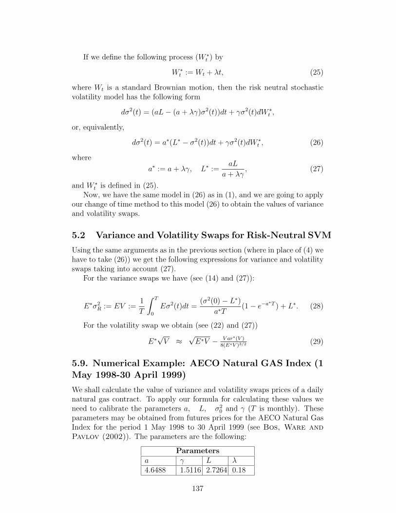
If we define the following process (W ∗t ) by

W ∗t := Wt + λt, (25)

where Wt is a standard Brownian motion, then the risk neutral stochasticvolatility model has the following form

dσ2(t) = (aL− (a+ λγ)σ2(t))dt+ γσ2(t)dW ∗t ,

or, equivalently,

dσ2(t) = a∗(L∗ − σ2(t))dt+ γσ2(t)dW ∗t , (26)

where

a∗ := a+ λγ, L∗ :=aL

a+ λγ, (27)

and W ∗t is defined in (25).

Now, we have the same model in (26) as in (1), and we are going to applyour change of time method to this model (26) to obtain the values of varianceand volatility swaps.

5.2 Variance and Volatility Swaps for Risk-Neutral SVM

Using the same arguments as in the previous section (where in place of (4) wehave to take (26)) we get the following expressions for variance and volatilityswaps taking into account (27).

For the variance swaps we have (see (14) and (27)):

E∗σ2R := EV :=

1

T

∫ T

0

Eσ2(t)dt =(σ2(0)− L∗)

a∗T(1− e−a∗T ) + L∗. (28)

For the volatility swap we obtain (see (22) and (27))

E∗√V ≈

√E∗V − V ar∗(V )

8(E∗V )3/2(29)

5.9. Numerical Example: AECO Natural GAS Index (1May 1998-30 April 1999)

We shall calculate the value of variance and volatility swaps prices of a dailynatural gas contract. To apply our formula for calculating these values weneed to calibrate the parameters a, L, σ2

0 and γ (T is monthly). Theseparameters may be obtained from futures prices for the AECO Natural GasIndex for the period 1 May 1998 to 30 April 1999 (see Bos, Ware andPavlov (2002)). The parameters are the following:

Parametersa γ L λ4.6488 1.5116 2.7264 0.18

137

For variance swap we use formula (14) and for volatility swap we use formula(22).

From this table we can calculate the values for risk adjusted parametersa∗ and L∗ :

a∗ = a+ λγ = 4.9337,

and

L∗ =aL

a+ λγ= 2.5690.

For the value of σ2(0) we can take σ2(0) = 2.25.For variance swap and for volatility swap with risk adjusted papameters

we use formula (28) and (29), respectively.

Appendix: Figures

Figure 1 depicts variance swap (price vs. maturity) for AECO Natural GasIndex (1 May 1998 to 30 April 1999), using formula (14).

Figure 2 depicts volatility swap (price vs. maturity) for AECO NaturalGas Index (1 May 1998 to 30 April 1999), using formula (22).

Figure 3 depicts varinace swap with risk adjusted parameters (price vs.maturity) for AECO Natural Gas Index (1 May 1998 to 30 April 1999), usingformula (28).

Figure 4 depicts volatility swap with risk adjusted parameters (price vs.maturity) for AECO Natural Gas Index (1 May 1998 to 30 April 1999), usingformula (29).

Figure 5 depicts comparison of adjusted (green line) and non-adjustedprice (red line) (naive strike vs. adjusted strike).

Figure 6 depicts convexity adjustment. It’s decreasing with swap matu-rity (the volatility of volatility over a long period of time is low).

138

Fig. 1: Variance Swap Fig. 2: Volatility Swap

Fig. 3: Variance Swap (Risk

Adjusted Parameters)

Fig. 4: Volatility Swap (Risk

Adjusted Parameters)

Fig. 5: Comparison: Adjusted

and Non-Adjusted Price

Fig. 6: Convexity Adjustment

139

References

L. P. Bos, A. F. Ware and B. S. Pavlov (2002): On a semi-spectralmethod for pricing an option on a mean-reverting asset, Quantitative Fi-nance, Volume 2, 337-345.

F. Black (1976): The pricing of commodity contracts, J. Financial Eco-nomics, 3, 167-179.

P. Carr and L. Wu (2009): Variance risk premia, Review of FinancialStudies 22, 1311-1341

O. Brockhaus and D. Long (2000): Volatility swaps made simple, RiskMagazine, January, 2000.

R. Elliott (1982): Stochastic Calculus and Applications, Springer-Verlag,New York.

C. Erb and C. Harvey (2006): The strategic and tactical value of com-modity futures. Financial Analysts J. 62, 69-97.

G. Gorton and G. Rouwenhorst (2006): Facts and fantasies aboutcommodity futures. Financial Analysts J. 62, 47-68.

Ibbotson (2006): Strategic asset allocation and commodities. March 27.

N. Ikeda and S. Watanabe (1981): Stochastic Differential Equationsand Diffusion Processes, Kodansha Ltd., Tokyo.

A. Javaheri, P. Wilmott and E. Haug (2002): GARCH and volatilityswaps, Wilmott Magazine, January.

H. Kan and R. Oomen (2007): What every investor should know aboutcommodities, Part I. J. of Investment Management 5, 4-28.

H. Kan and R. Oomen (2007): What every investor should know aboutcommodities, Part I. J. of Investment Management 5, 29-64.

D. Lamperton and B. Lapeyre (1996): Introduction to Stochastic Cal-culus Applied to Finance, Chapmann & Hall.

D. Pilipovic (1998): Energy Risk. Valuing and Managing Energy Deriva-tives, New York, McGraw-Hill.

E. Schwartz (1997): The stochastic behaviour of commodity prices: im-plications for pricing and hedging, J. Finance, 52, 923-973.

A. Swishchuk (2004): Modeling and valuing of variance and volatilityswaps for financial markets with stochastic volatilities, Wilmott Magazine,Technical Article No2, September Issue, 64-72.

140

A. Swishchuk (2013): Variance and volatility swaps in energy markets.Journal of Energy Markets. 6(1): 33-49.

A. Trolle and E. Schwartz (2010): Varinace risk premia in energycommodities, J. of Derivatives, Spring, v. 17, No. 3, 15-32.

P. Wilmott, S. Howison and J. Dewynne (1995): The Mathematicsof Financial Derivatives, Cambridge, Cambridge University Press.

P. Wilmott (2000): Paul Wilmott on Quantitative Finance, New York,Wiley.

141

Epilogue

’Time you enjoy wasting, was not wasted’,-John Lennon.

The present book was devoted to the history of change of time meth-ods (CTM), connection of CTM with stochastic volatilities and finance, andmany applications of CTM. As a reader may noticed, this book is a briefintroduction to the theory of CTM and may be considered as a handbook inthis area.

I hope that you enjoyed your time while reading this book, and thankyou for getting to this very end.

142