Embed Size (px)
Citation preview

Algorithmic and High-Frequency Trading
A Primer on the Microstructure of Financial Markets
Julia Schmidt
LOBSTER June 2nd 2016

A Primer on the Microstructure of Financial Markets
Overview
� Introduction� Market Making
— Grossman-Miller Market Making Model— Trading Costs— Measuring Liquidity— Market Making using Limit Orders
� Trading on an Informational Advantage� MM with an Informational Disadvantage
— Price Dynamics— Price Sensitive Liquidity Traders
A Primer on the Microstructure of Financial Markets
Introduction
� Market Microstructure— subfield of finance— “study of the process and outcome of exchanging assets under explicit
trading rules” (O’Hara(1995))� Key Dimension of trading and pricing: Information � Price Efficiency
— “market prices are an efficient way of transmitting the information required to arrive at a Pareto optimal allocation of resources” (Grossman&Stiglitz (1976))
� Trading: many possible ways— focus on trading in large electronic markets

A Primer on the Microstructure of Financial Markets
Overview
� Introduction� Market Making
— Grossman-Miller Market Making Model— Trading Costs— Measuring Liquidity— Market Making using Limit Orders
� Trading on an Informational Advantage� MM with an Informational Disadvantage
— Price Dynamics— Price Sensitive Liquidity Traders
A Primer on the Microstructure of Financial Markets
Market Making
� Market participants— Market Maker (MM)— Liquidity Trader (LT)
� Market Maker— Competition— Provide liquidity Æ immediacy— Bid and ask prices Æ Limit Orders
� Liquidity Trader— Take liquidity

A Primer on the Microstructure of Financial Markets
Overview
� Introduction� Market Making
— Grossman-Miller Market Making Model— Trading Costs— Measuring Liquidity— Market Making using Limit Orders
� Trading on an Informational Advantage� MM with an Informational Disadvantage
— Price Dynamics— Price Sensitive Liquidity Traders
A Primer on the Microstructure of Financial Markets
Grossman-Miller Market Making Model
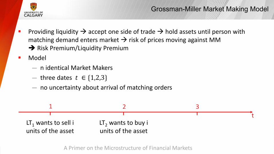
� Providing liquidity Æ accept one side of trade Æ hold assets until person with matching demand enters market Æ risk of prices moving against MMÎ Risk Premium/Liquidity Premium
� Model— n identical Market Makers— three dates 𝑡 ∈ {1,2,3}— no uncertainty about arrival of matching orders
t1 32
LT1 wants to sell iunits of the asset
LT2 wants to buy iunits of the asset
A Primer on the Microstructure of Financial Markets
Grossman-Miller Market Making Model
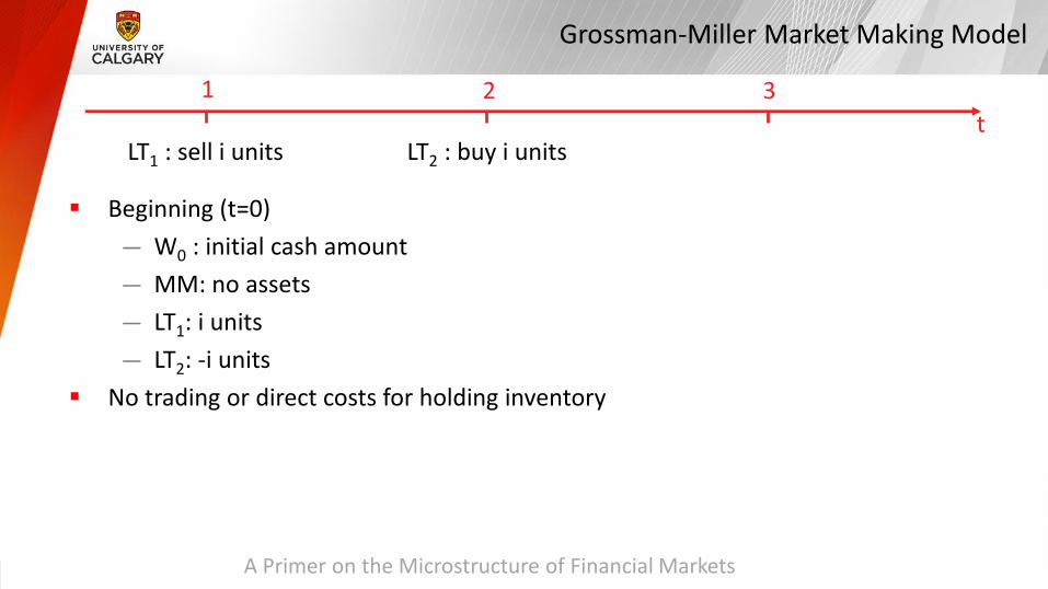
� Beginning (t=0)— W0 : initial cash amount — MM: no assets— LT1: i units— LT2: -i units
� No trading or direct costs for holding inventory
t1 32
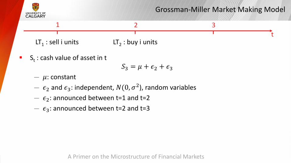
LT1 : sell i units LT2 : buy i units
A Primer on the Microstructure of Financial Markets
Grossman-Miller Market Making Model
� St : cash value of asset in t𝑆3 = 𝜇 + 𝜖2 + 𝜖3
— 𝜇: constant— 𝜖2 and 𝜖3: independent, 𝑁(0, 𝜎2), random variables— 𝜖2: announced between t=1 and t=2— 𝜖3: announced between t=2 and t=3
t1 32
LT1 : sell i units LT2 : buy i units
A Primer on the Microstructure of Financial Markets
Grossman-Miller Market Making Model
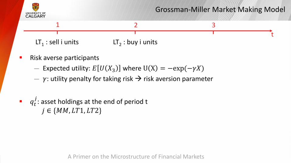
� Risk averse participants— Expected utility: 𝐸 𝑈 𝑋3 where U X = −exp(−𝛾𝑋)— 𝛾: utility penalty for taking risk Æ risk aversion parameter
� 𝑞𝑡𝑗: asset holdings at the end of period t 𝑗 ∈ {𝑀𝑀, 𝐿𝑇1, 𝐿𝑇2}
t1 32
LT1 : sell i units LT2 : buy i units
A Primer on the Microstructure of Financial Markets
Grossman-Miller Market Making Model
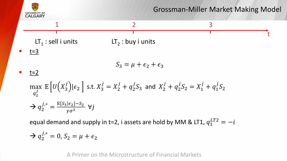
� t=3
𝑆3 = 𝜇 + 𝜖2 + 𝜖3� t=2
max𝑞2𝑗
𝔼 𝑈 𝑋3𝑗 |𝜖2 s.t. 𝑋3
𝑗 = 𝑋2𝑗 + 𝑞2
𝑗𝑆3 and 𝑋2𝑗 + 𝑞2
𝑗𝑆2 = 𝑋1𝑗 + 𝑞1
𝑗𝑆2
Æ 𝑞2𝑗,∗ = 𝔼 𝑆3 𝜖2]−𝑆2
𝛾𝜎2∀𝑗
equal demand and supply in t=2, i assets are hold by MM & LT1, 𝑞1𝐿𝑇2 = −𝑖
Æ 𝑞2𝑗,∗ = 0, 𝑆2 = 𝜇 + 𝜖2
t1 32
LT1 : sell i units LT2 : buy i units
A Primer on the Microstructure of Financial Markets
Grossman-Miller Market Making Model
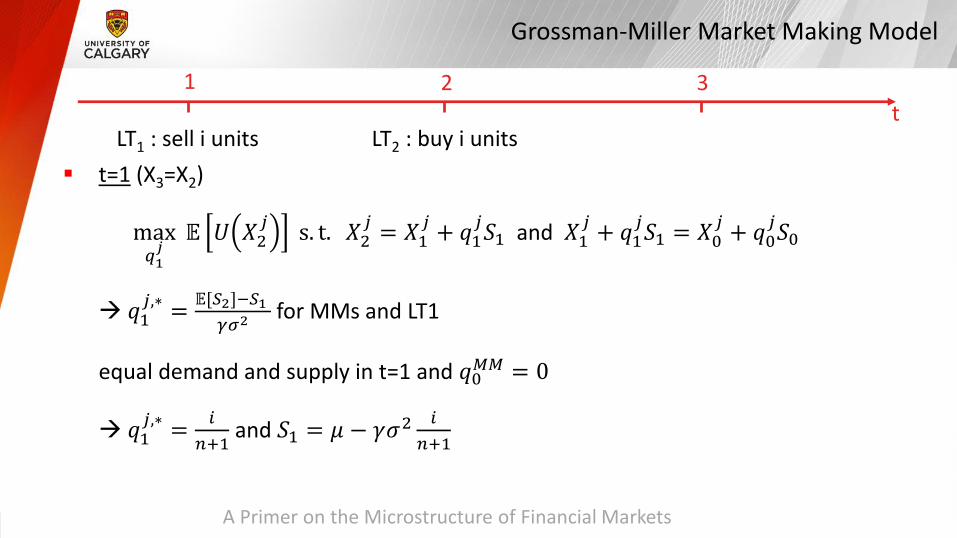
� t=1 (X3=X2)
max𝑞1𝑗
𝔼 𝑈 𝑋2𝑗 s. t. 𝑋2
𝑗 = 𝑋1𝑗 + 𝑞1
𝑗𝑆1 and 𝑋1𝑗 + 𝑞1
𝑗𝑆1 = 𝑋0𝑗 + 𝑞0
𝑗𝑆0
Æ 𝑞1𝑗,∗ = 𝔼[𝑆2]−𝑆1
𝛾𝜎2for MMs and LT1
equal demand and supply in t=1 and 𝑞0𝑀𝑀 = 0
Æ 𝑞1𝑗,∗ = 𝑖
𝑛+1and 𝑆1 = 𝜇 − 𝛾𝜎2 𝑖
𝑛+1
t1 32
LT1 : sell i units LT2 : buy i units
A Primer on the Microstructure of Financial Markets
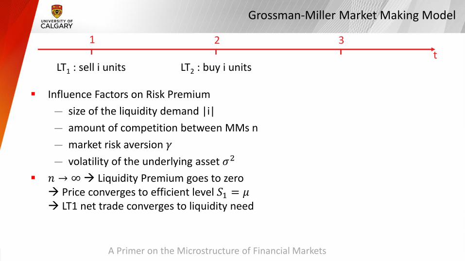
Grossman-Miller Market Making Model
� Influence Factors on Risk Premium— size of the liquidity demand |i|— amount of competition between MMs n— market risk aversion 𝛾— volatility of the underlying asset 𝜎2
� 𝑛 → ∞Æ Liquidity Premium goes to zero Æ Price converges to efficient level 𝑆1 = 𝜇Æ LT1 net trade converges to liquidity need
t1 32
LT1 : sell i units LT2 : buy i units

A Primer on the Microstructure of Financial Markets
Overview
� Introduction� Market Making
— Grossman-Miller Market Making Model— Trading Costs— Measuring Liquidity— Market Making using Limit Orders
� Trading on an Informational Advantage� MM with an Informational Disadvantage
— Price Dynamics— Price Sensitive Liquidity Traders
A Primer on the Microstructure of Financial Markets
Trading Costs
� Model with participation costs c— c : proxy for time and investments needed to keep a constant, active and
competitive presence in the market + opportunity costs— Result:
� Level of competition decreases monotonically with supplier’s participation costs
Æ Increase the liquidity premium
A Primer on the Microstructure of Financial Markets
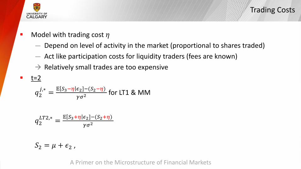
Trading Costs
� Model with trading cost 𝜂— Depend on level of activity in the market (proportional to shares traded)— Act like participation costs for liquidity traders (fees are known)Æ Relatively small trades are too expensive
� t=2
𝑞2𝑗,∗ = 𝔼 𝑆3−𝜂 𝜖2]−(𝑆2−𝜂)
𝛾𝜎2for LT1 & MM
𝑞2𝐿𝑇2,∗ = 𝔼 𝑆3+𝜂 𝜖2]−(𝑆2+𝜂)
𝛾𝜎2
𝑆2 = 𝜇 + 𝜖2 ,
A Primer on the Microstructure of Financial Markets
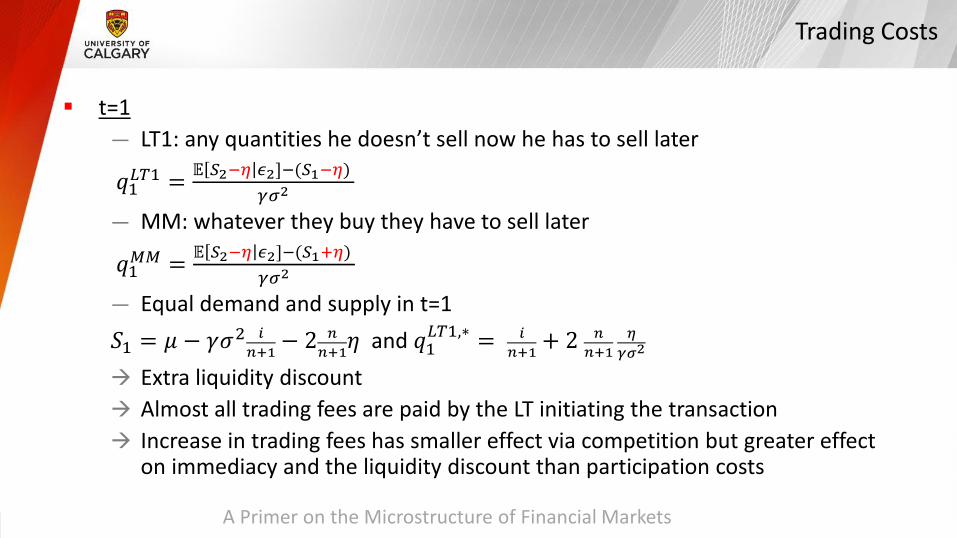
Trading Costs
� t=1— LT1: any quantities he doesn’t sell now he has to sell later
𝑞1𝐿𝑇1 =𝔼 𝑆2−𝜂 𝜖2]−(𝑆1−𝜂)
𝛾𝜎2
— MM: whatever they buy they have to sell later
𝑞1𝑀𝑀 = 𝔼 𝑆2−𝜂 𝜖2]−(𝑆1+𝜂)𝛾𝜎2
— Equal demand and supply in t=1 𝑆1 = 𝜇 − 𝛾𝜎2 𝑖
𝑛+1 − 2 𝑛𝑛+1𝜂 and 𝑞1
𝐿𝑇1,∗ = 𝑖𝑛+1 + 2 𝑛
𝑛+1𝜂
𝛾𝜎2
Æ Extra liquidity discount Æ Almost all trading fees are paid by the LT initiating the transactionÆ Increase in trading fees has smaller effect via competition but greater effect
on immediacy and the liquidity discount than participation costs

A Primer on the Microstructure of Financial Markets
Overview
� Introduction� Market Making
— Grossman-Miller Market Making Model— Trading Costs— Measuring Liquidity— Market Making using Limit Orders
� Trading on an Informational Advantage� MM with an Informational Disadvantage
— Price Dynamics— Price Sensitive Liquidity Traders
A Primer on the Microstructure of Financial Markets
Measuring Liquidity
� Transformation to electronic asset markets— Trading does not take place at once and not to a single price— LT post MO into exchange Æmeet LO of MM, which are resting in LOB— Here:
� LT1’s MO enters market and is executed against LO in LOB� Possibilities: one large order or many small orders� As execution price changes, so does LT1’s strategy and eventually, after
selling 𝑖 𝑛𝑛+1
shares, the price has moved too far and LT1 stops trading
� Overall: execution at average price S1
� Risk premium: S1 – midprice of first MO
A Primer on the Microstructure of Financial Markets
Measuring Liquidity
� Effect of traded quantity Æ Rewrite S1𝑆1 = 𝜇 + 𝜆𝑞𝐿𝑇1
� Grossman-Miller model:𝜆 = − 1
𝑛𝛾𝜎2 and 𝑞𝐿𝑇1 = 𝑖 𝑛
𝑛+1— 𝜆 : market price reaction to LT1’s total order (price impact)— Describes liquidity of the market for this asset — The more liquid, the lower the absolute lambda
A Primer on the Microstructure of Financial Markets
Measuring Liquidity
� Other way to measure liquidity: autocovariance in asset price changes (or returns)� Introduce new date t=0 and a random public event 𝜖1 announced between 0 and 1
— 𝑆3 = 𝜇 + 𝜖1 + 𝜖2 + 𝜖3— 𝜇0 = 𝔼 𝑆3 , 𝜇1= 𝔼 𝑆3 𝜖1 , 𝜇2 = 𝔼 𝑆3 𝜖1, 𝜖2 , 𝜇3 = 𝑆3— 𝜖1, 𝜖2, 𝜖3 i.i.d. ~𝑁(0, 𝜎2)— Discrete process 𝜇𝑡 is a martingale, efficient price process— No trades in t=0 Æ 𝑆0 = 𝔼 𝑆3 = 𝜇0— 𝑆1 = 𝜇 + 𝜆𝑞𝐿𝑇1, 𝑆2 = 𝜇2— Δ1 = 𝑆1 − 𝑆0, Δ2 = 𝑆2 − 𝑆1Æ 𝐶𝑜𝑣 Δ1, Δ2 = −𝜆2𝑉𝑎𝑟 𝑞𝐿𝑇1 < 0Æ Autocovariance captures liquidity just like price impact doesÆ 𝜆 → 0Æ 𝐶𝑜𝑣 → 0Æ price process converges to martingale process 𝜇𝑡

A Primer on the Microstructure of Financial Markets
Overview
� Introduction� Market Making
— Grossman-Miller Market Making Model— Trading Costs— Measuring Liquidity— Market Making using Limit Orders
� Trading on an Informational Advantage� MM with an Informational Disadvantage
— Price Dynamics— Price Sensitive Liquidity Traders
A Primer on the Microstructure of Financial Markets
Market Making using Limit Orders
� Small risk-neutral trader with costless inventory management and infinite patience� Other MMs do not react to our MMs decision � Don‘t know time and size of incoming MOs� 𝑆𝑡: current value of asset, midprice� Liquidates her inventory at midprice at no costs
� 𝛿±: depth, distance from mid price� 𝑝±: probability that an MO arrives � 𝑃±: cdf, probability that price walks to MM‘s LO after arrival of MOÆ 𝑝−𝑃−(𝛿−): prob that buy LO is filled� Distribution of other LO’s: exponential with parameter 𝜅±Æ
𝑝−𝑃−(𝛿−) = 𝑝−𝑒−𝜅−𝛿−

A Primer on the Microstructure of Financial Markets
Market Making using Limit Orders
� Π: MM‘s profit per trade
max𝛿+,𝛿−
𝔼[Π (𝛿+, 𝛿−)] = max𝛿+,𝛿−
{𝑝+𝑒−𝜅+𝛿+𝛿+ + 𝑝−𝑒−𝜅−𝛿−𝛿−}
Æ 𝛿±,∗ = 1𝜅±
� Given our parametric choice of 𝑃±, the optimal depth is equal to the mean depthin the LOB
A Primer on the Microstructure of Financial Markets
Overview
� Introduction� Market Making
— Grossman-Miller Market Making Model— Trading Costs— Measuring Liquidity— Market Making using Limit Orders
� Trading on an Informational Advantage� MM with an Informational Disadvantage
— Price Dynamics— Price Sensitive Liquidity Traders
A Primer on the Microstructure of Financial Markets
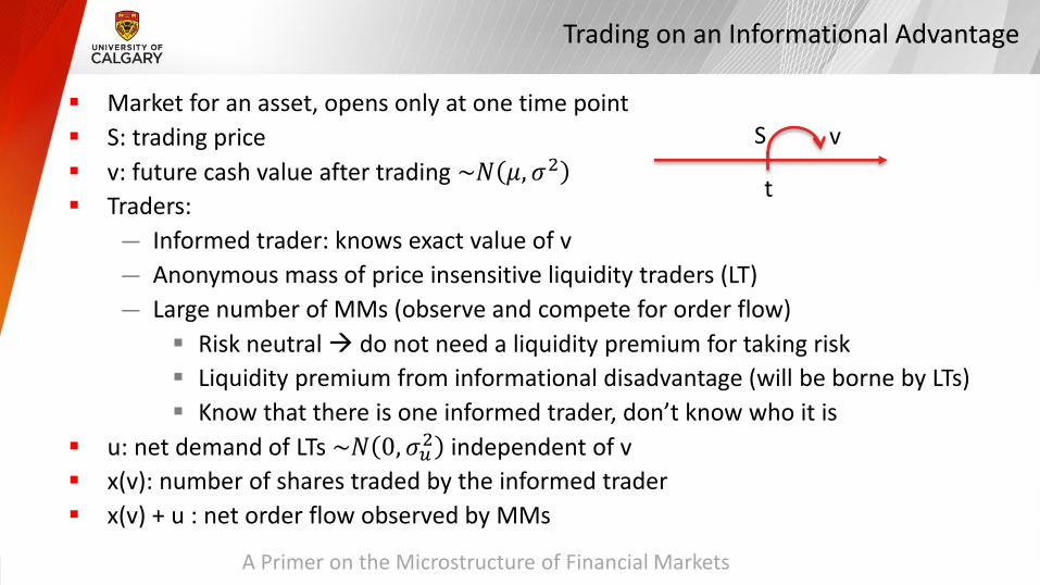
Trading on an Informational Advantage
� Market for an asset, opens only at one time point� S: trading price� v: future cash value after trading ~𝑁 𝜇, 𝜎2
� Traders: — Informed trader: knows exact value of v— Anonymous mass of price insensitive liquidity traders (LT)— Large number of MMs (observe and compete for order flow)
� Risk neutral Æ do not need a liquidity premium for taking risk� Liquidity premium from informational disadvantage (will be borne by LTs)� Know that there is one informed trader, don’t know who it is
� u: net demand of LTs ~𝑁 0, 𝜎𝑢2 independent of v� x(v): number of shares traded by the informed trader� x(v) + u : net order flow observed by MMs
t
S v
A Primer on the Microstructure of Financial Markets
Trading on an Informational Advantage
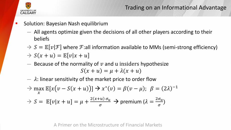
� Solution: Bayesian Nash equilibrium — All agents optimize given the decisions of all other players according to their
beliefsÆ 𝑆 = 𝔼 𝑣 ℱ where ℱ:all information available to MMs (semi-strong efficiency)Æ 𝑆 𝑥 + 𝑢 = 𝔼 𝑣 𝑥 + 𝑢— Because of the normality of 𝑣 and u insiders hypothesize
𝑆 𝑥 + 𝑢 = 𝜇 + 𝜆(𝑥 + 𝑢)— 𝜆: linear sensitivity of the market price to order flow
Æmax𝑥
𝔼[𝑥 𝑣 − 𝑆 𝑥 + 𝑢 ]Æ 𝑥∗ 𝑣 = 𝛽 𝑣 − 𝜇 ; 𝛽 = 2𝜆 −1
Æ 𝑆 = 𝔼[𝑣|𝑥 + 𝑢] = 𝜇 + 2 𝑥+𝑢 𝜎𝑢𝜎
Æ premium (𝜆 = 2𝜎𝑢𝜎)

A Primer on the Microstructure of Financial Markets
Overview
� Introduction� Market Making
— Grossman-Miller Market Making Model— Trading Costs— Measuring Liquidity— Market Making using Limit Orders
� Trading on an Informational Advantage� MM with an Informational Disadvantage
— Price Dynamics— Price Sensitive Liquidity Traders
A Primer on the Microstructure of Financial Markets
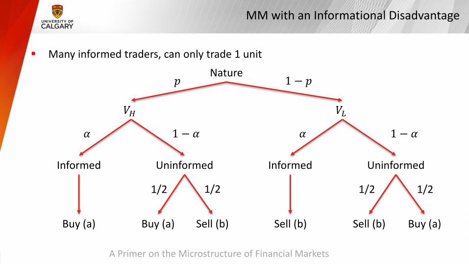
MM with an Informational Disadvantage
� Many informed traders, can only trade 1 unit Nature
Informed InformedUninformed Uninformed
𝑉𝐻 𝑉𝐿
𝛼 1 − 𝛼𝛼1 − 𝛼
Buy (a) Sell (b) Buy (a)Buy (a) Sell (b)Sell (b)
1/2 1/2 1/2 1/2
𝑝 1 − 𝑝
A Primer on the Microstructure of Financial Markets
MM with an Informational Disadvantage
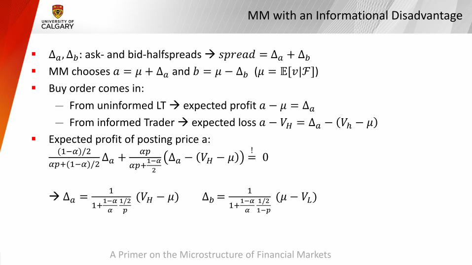
� Δ𝑎, Δ𝑏: ask- and bid-halfspreadsÆ 𝑠𝑝𝑟𝑒𝑎𝑑 = Δ𝑎 + Δ𝑏� MM chooses 𝑎 = 𝜇 + Δ𝑎 and 𝑏 = 𝜇 − Δ𝑏 (𝜇 = 𝔼[𝑣|ℱ])� Buy order comes in:
— From uninformed LT Æ expected profit 𝑎 − 𝜇 = Δ𝑎— From informed Trader Æ expected loss 𝑎 − 𝑉𝐻 = Δ𝑎 − 𝑉ℎ − 𝜇
� Expected profit of posting price a:(1−𝛼)/2
𝛼𝑝+(1−𝛼)/2Δ𝑎 +
𝛼𝑝𝛼𝑝+1−𝛼
2Δ𝑎 − 𝑉𝐻 − 𝜇 =
!0
Æ Δ𝑎 =1
1+1−𝛼𝛼
1/2𝑝
(𝑉𝐻 − 𝜇) Δ𝑏 =1
1+1−𝛼𝛼
1/21−𝑝
(𝜇 − 𝑉𝐿)
A Primer on the Microstructure of Financial Markets
Overview
� Introduction� Market Making
— Grossman-Miller Market Making Model— Trading Costs— Measuring Liquidity— Market Making using Limit Orders
� Trading on an Informational Advantage� MM with an Informational Disadvantage
— Price Dynamics— Price Sensitive Liquidity Traders
A Primer on the Microstructure of Financial Markets
Price Dynamics
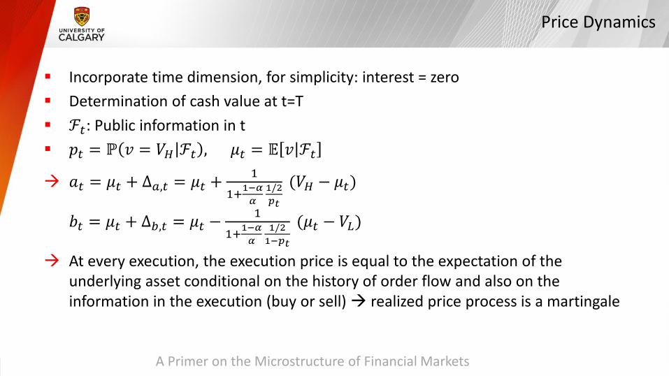
� Incorporate time dimension, for simplicity: interest = zero � Determination of cash value at t=T� ℱ𝑡: Public information in t� 𝑝𝑡 = ℙ 𝑣 = 𝑉𝐻 ℱ𝑡 , 𝜇𝑡 = 𝔼 𝑣 ℱ𝑡
Æ 𝑎𝑡 = 𝜇𝑡 + Δ𝑎,𝑡 = 𝜇𝑡 +1
1+1−𝛼𝛼
1/2𝑝𝑡
(𝑉𝐻 − 𝜇𝑡)
𝑏𝑡 = 𝜇𝑡 + Δ𝑏,𝑡 = 𝜇𝑡 −1
1+1−𝛼𝛼
1/21−𝑝𝑡
(𝜇𝑡 − 𝑉𝐿)
Æ At every execution, the execution price is equal to the expectation of the underlying asset conditional on the history of order flow and also on the information in the execution (buy or sell) Æ realized price process is a martingale

A Primer on the Microstructure of Financial Markets
Overview
� Introduction� Market Making
— Grossman-Miller Market Making Model— Trading Costs— Measuring Liquidity— Market Making using Limit Orders
� Trading on an Informational Advantage� MM with an Informational Disadvantage
— Price Dynamics— Price Sensitive Liquidity Traders
A Primer on the Microstructure of Financial Markets
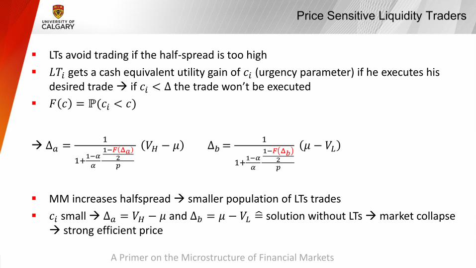
Price Sensitive Liquidity Traders
� LTs avoid trading if the half-spread is too high� 𝐿𝑇𝑖 gets a cash equivalent utility gain of 𝑐𝑖 (urgency parameter) if he executes his
desired trade Æ if 𝑐𝑖 < Δ the trade won’t be executed � 𝐹 𝑐 = ℙ(𝑐𝑖 < 𝑐)
Æ Δ𝑎 =1
1+1−𝛼𝛼
1−𝐹 Δ𝑎2𝑝
𝑉𝐻 − 𝜇 Δ𝑏 =1
1+1−𝛼𝛼
1−𝐹 Δ𝑏2𝑝
𝜇 − 𝑉𝐿
� MM increases halfspreadÆ smaller population of LTs trades� 𝑐𝑖 small Æ Δ𝑎 = 𝑉𝐻 − 𝜇 and Δ𝑏 = 𝜇 − 𝑉𝐿 = solution without LTs Æmarket collapseÆ strong efficient price

A Primer on the Microstructure of Financial Markets
Thank you -