Embed Size (px)
Citation preview

Change Detection in Precision Manufacturing Processes under Transient Conditions
Zimo Wang Ph.D. candidate [email protected]
Fourth Texas Educators Conference on Machining
Zimo (Robin) Wang, Satish T.S. Bukkapatnam
School of Industrial Engineering and Management, Oklahoma State University
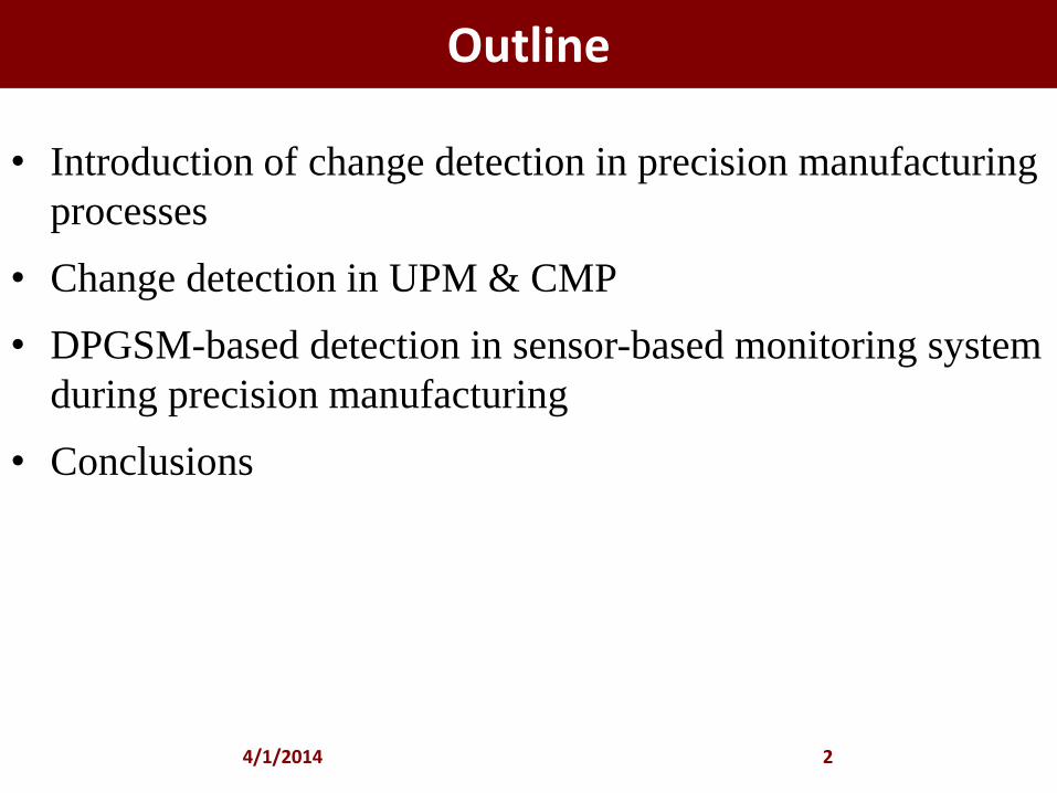
Outline
• Introduction of change detection in precision manufacturing
processes
• Change detection in UPM & CMP
• DPGSM-based detection in sensor-based monitoring system
during precision manufacturing
• Conclusions
4/1/2014 2
Introduction
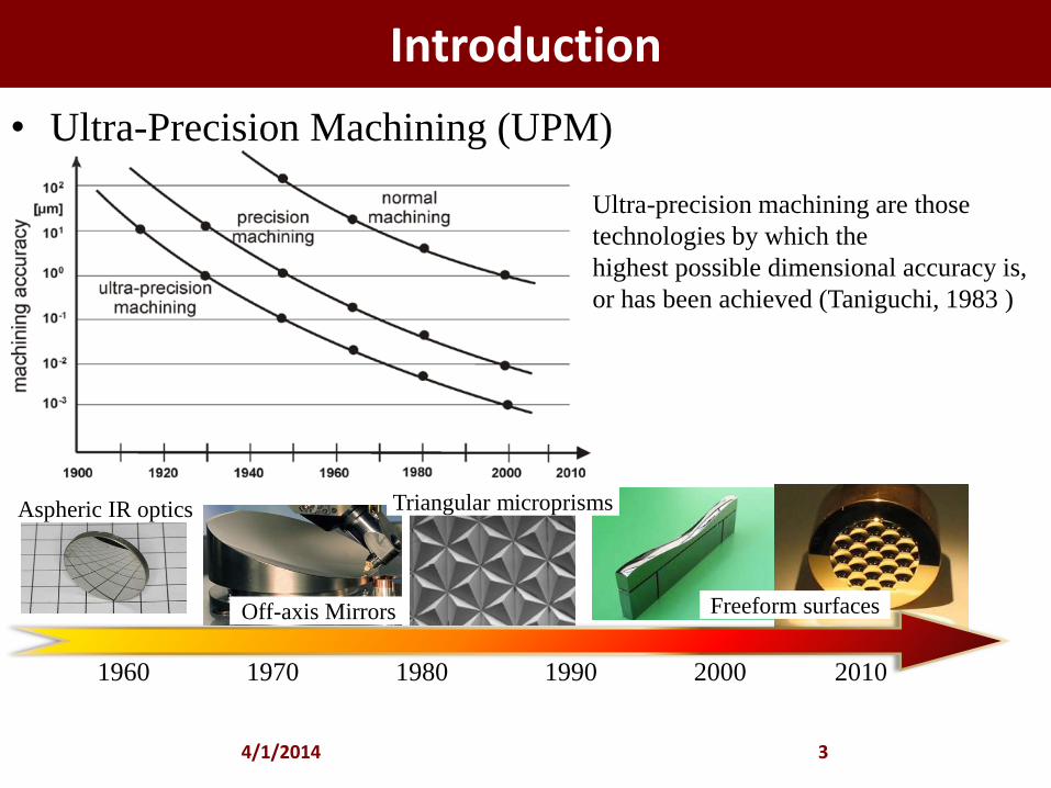
Aspheric IR optics
1960 1970 1980 1990 2000 2010
Off-axis Mirrors Freeform surfaces
Triangular microprisms
Ultra-precision machining are those
technologies by which the
highest possible dimensional accuracy is,
or has been achieved (Taniguchi, 1983 )
• Ultra-Precision Machining (UPM)
4/1/2014 3
Introduction
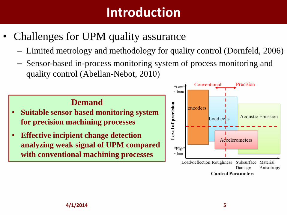
• Challenges for UPM quality assurance – Limited metrology and methodology for quality control (Dornfeld, 2006)
– Sensor-based in-process monitoring system of process monitoring and
quality control (Abellan-Nebot, 2010)
4/1/2014 5
Demand • Suitable sensor based monitoring system
for precision machining processes
• Effective incipient change detection
analyzing weak signal of UPM compared
with conventional machining processes

Surface defects in ultra-precision machining
• System vibrations
– Chatter: tool, toolholder and spindle together vibrate at some natural
frequency
– Scratches on the surface, ruining the geometric acquirement of product
4/1/2014 6
One important effect that is not considered in the model above is built up edge. Under most cutting
conditions, some of the cut material will attach to the cutting point. This tends to cause the cut to be
deeper than the tip of the cutting tool and degrades surface finish. Also, periodically the built up
edge will break off and remove some of the cutting tool. Thus, tool life is reduced. In general, built
up edge can be reduced by:Increasing cutting speed
Decreasing feed rate
Increasing ambient workpiece temperature
Increasing rake angle
Reducing friction (by applying cutting fluid)
Rippled surface finish
Most common surface defects (e.g. surface scratches and variations) are
due to abnormal vibration (e.g. chatters) and built-up edge (BUE)
Scratch
Surface defects in ultra-precision machining
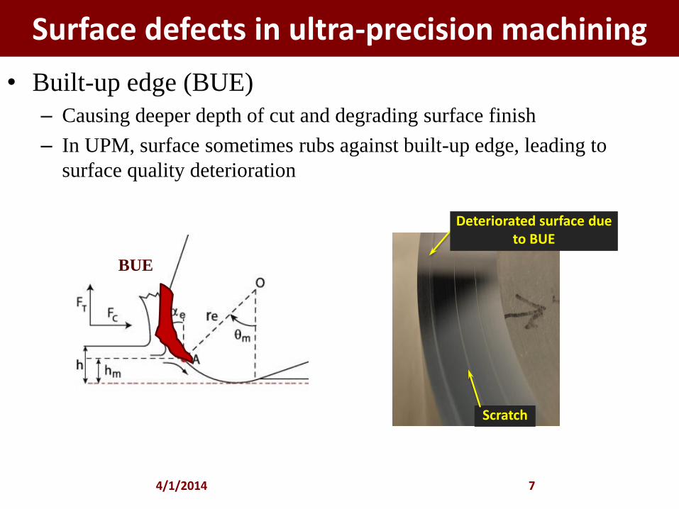
• Built-up edge (BUE)
– Causing deeper depth of cut and degrading surface finish
– In UPM, surface sometimes rubs against built-up edge, leading to
surface quality deterioration
4/1/2014 7
BUE
Mean Ra
Region 1 51nm
Region 2 49nm
Region 3 40nm
Scratch
Deteriorated surface due to BUE
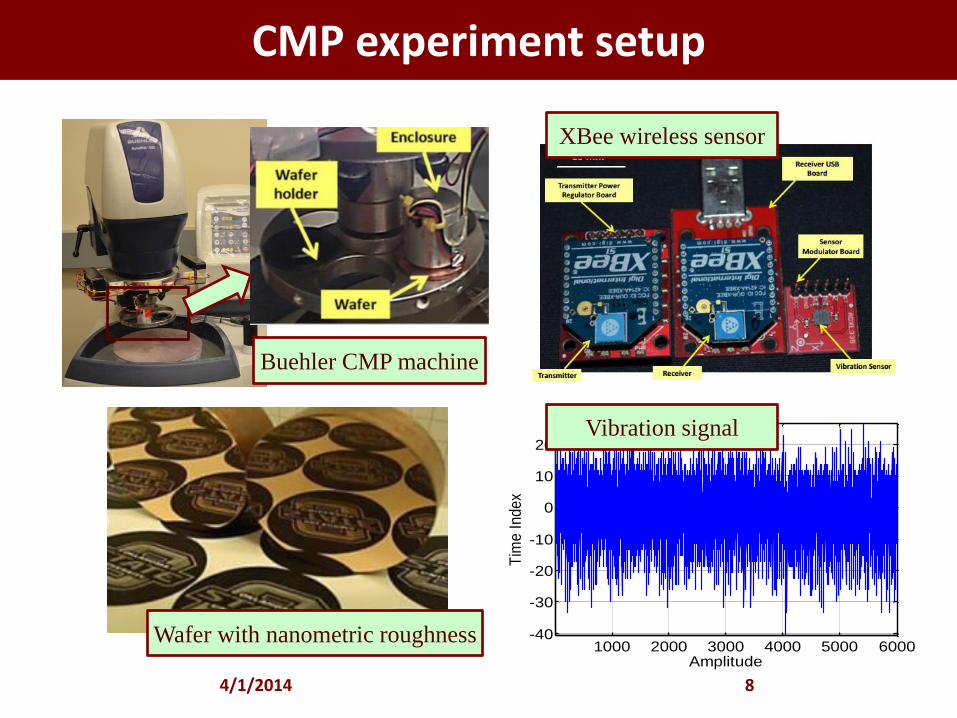
CMP experiment setup
4/1/2014 8
1000 2000 3000 4000 5000 6000-40
-30
-20
-10
0
10
20
Tim
e I
nd
ex
Amplitude
XBee wireless sensor
Buehler CMP machine
Vibration signal
Wafer with nanometric roughness
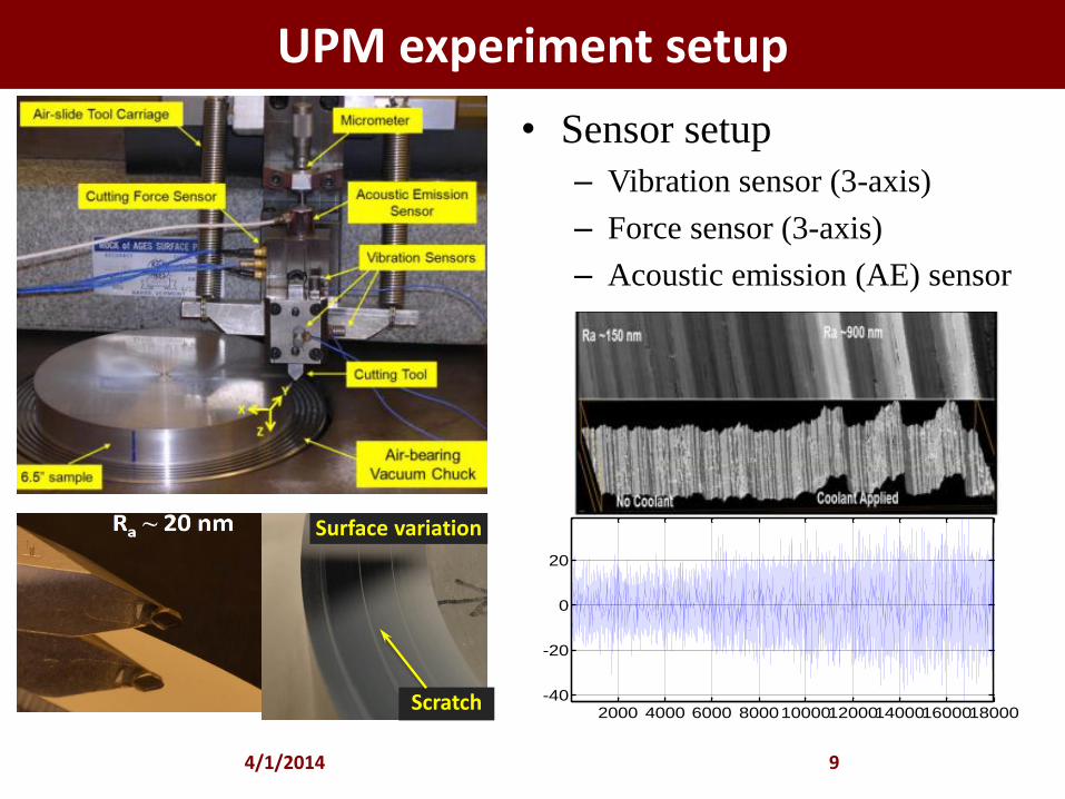
UPM experiment setup
• Sensor setup
– Vibration sensor (3-axis)
– Force sensor (3-axis)
– Acoustic emission (AE) sensor
4/1/2014 9
Scratch
Surface variation
2000 4000 6000 80001000012000140001600018000-40
-20
0
20
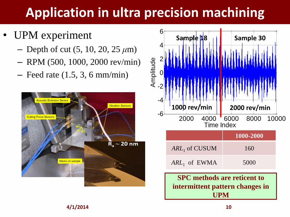
Application in ultra precision machining
• UPM experiment
– Depth of cut (5, 10, 20, 25 μm)
– RPM (500, 1000, 2000 rev/min)
– Feed rate (1.5, 3, 6 mm/min)
4/1/2014 10
2000 4000 6000 8000 10000-6
-4
-2
0
2
4
6
Am
plit
ud
e
Time Index
Sample 18 Sample 30
1000 rev/min 2000 rev/min
1000-2000
ARL1 of CUSUM 160
ARL1 of EWMA 5000
SPC methods are reticent to
intermittent pattern changes in
UPM
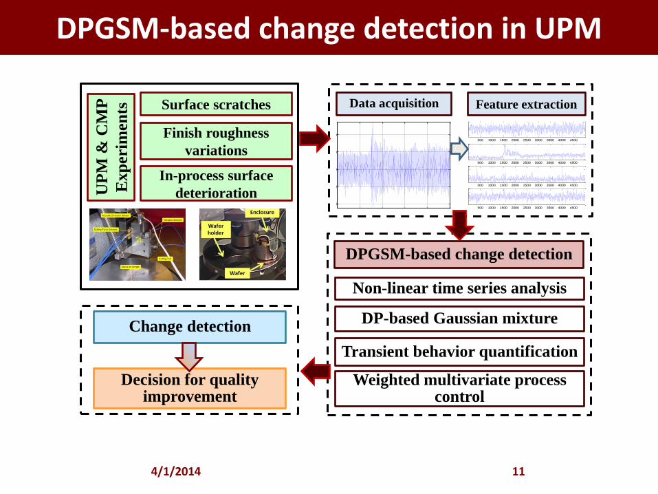
DPGSM-based change detection in UPM
4/1/2014 11
UP
M &
CM
P
Exp
erim
ents
Surface scratches
Finish roughness
variations
In-process surface
deterioration 1 2 3 4 5
x 104
-40
-20
0
20
40500 1000 1500 2000 2500 3000 3500 4000 4500
-1
0
1
500 1000 1500 2000 2500 3000 3500 4000 45005
10
15
500 1000 1500 2000 2500 3000 3500 4000 45002
4
6
500 1000 1500 2000 2500 3000 3500 4000 4500
-0.5
0
0.5
Data acquisition Feature extraction
Non-linear time series analysis
DPGSM-based change detection
DP-based Gaussian mixture
Transient behavior quantification
Weighted multivariate process control
Decision for quality improvement
Change detection
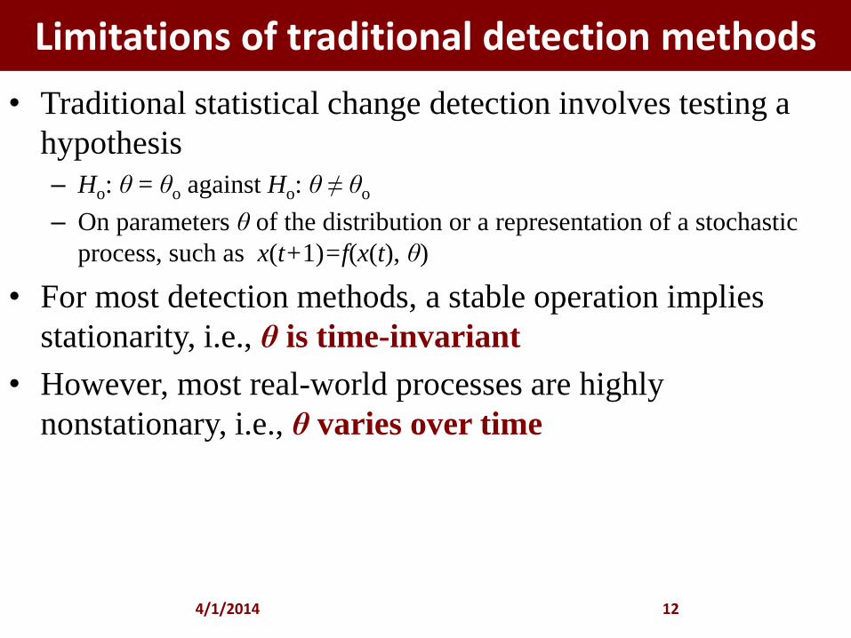
Limitations of traditional detection methods
• Traditional statistical change detection involves testing a
hypothesis
– Ho: θ = θo against Ho: θ ≠ θo
– On parameters θ of the distribution or a representation of a stochastic
process, such as x(t+1)=f(x(t), θ)
• For most detection methods, a stable operation implies
stationarity, i.e., θ is time-invariant
• However, most real-world processes are highly
nonstationary, i.e., θ varies over time
4/1/2014 12
From a statistical standpoint, change detection
process involves testing a hypothesis, H0: θ =
θ0 against H1: θ ≠ θ0 on the parameters θ of the
distribution or some other quantifiers of the
underlying state vector x.
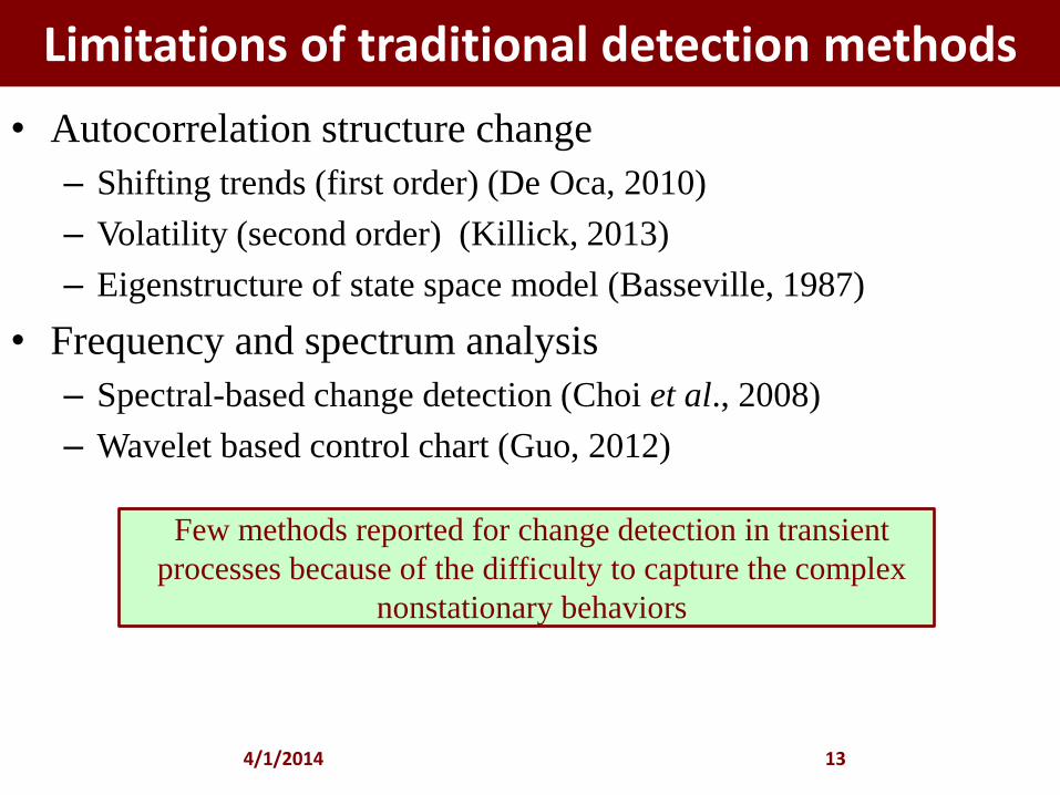
Limitations of traditional detection methods
• Autocorrelation structure change
– Shifting trends (first order) (De Oca, 2010)
– Volatility (second order) (Killick, 2013)
– Eigenstructure of state space model (Basseville, 1987)
• Frequency and spectrum analysis
– Spectral-based change detection (Choi et al., 2008)
– Wavelet based control chart (Guo, 2012)
4/1/2014 13
Few methods reported for change detection in transient
processes because of the difficulty to capture the complex
nonstationary behaviors
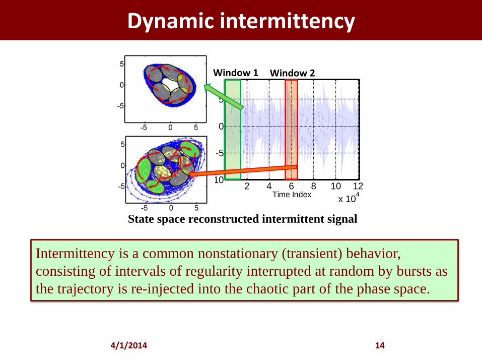
Dynamic intermittency
4/1/2014 14
Phase space for area-preserving map of intermittent signal
(Artuso, et al. 2003)
Intermittency is a common nonstationary (transient) behavior,
consisting of intervals of regularity interrupted at random by bursts as
the trajectory is re-injected into the chaotic part of the phase space.
2 4 6 8 10 12
x 104
-10
-5
0
5
Time Index
Am
plit
ud
e
Window 1 Window 2
State space reconstructed intermittent signal
𝜋11(1) ⋯ 𝜋15
(1) . . . 0⋮ ⋱ ⋮𝜋51(1)
⋮0
⋯𝜋55(1) … 0⋱ ⋮
0 … 0
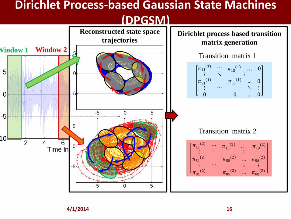
Dirichlet Process-based Gaussian State Machines (DPGSM)
4/1/2014 16
2 4 6 8 10 12
x 104
-10
-5
0
5
Am
plit
ud
e
Time Index
Window 1 Window 2
-5 0 5
-5
0
5
Y-A
XIS
X-AXIS
-5 0 5
-5
0
5
Y-A
XIS
X-AXIS
0.48 0.05 0.06 0.08 0.05 0.17 0.10 0.01
0.08 0.78 0.00 0.00 0.00 0.02 0.00 0.11
0.04 0.18 0.74 0.00 0.04 0.00 0.00 0.00
0.07 0.00 0.00 0.81 0.00 0.03 0.09 0.00
0.03 0.00 0.43 0.00 0.51 0.00 0.02 0.00
0.22 0.00 0.00 0.16 0.00 0.51 0.11 0.00
0.17 0.00 0.04 0.00 0.30 0.03 0.47 0.00
0.08 0.06 0.00 0.01 0.00 0.30 0.00 0.55
0.12 0.07 0.02 0.04 0.17 0.21 0.36 0.01
0.01 0.53 0.00 0.00 0.00 0.01 0.00 0.45
0.02 0.31 0.63 0.00 0.04 0.00 0.00 0.00
0.18 0.00 0.00 0.06 0.01 0.20 0.56 0.00
0.01 0.00 0.36 0.00 0.62 0.00 0.01 0.00
0.18 0.00 0.00 0.07 0.01 0.48 0.26 0.00
0.07 0.00 0.01 0.00 0.48 0.01 0.43 0.00
0.04 0.02 0.00 0.00 0.00 0.25 0.00 0.69
Reconstructed state space
trajectories
Show overall representation (show an
animation with a nonstionary (asceinding-
desceinding notes?) time series on left and the
state space on right, next fill the state space
with gaussian clusters and the transitions.
Next, show the time series evolving into a
different characterisitc. Now show the new
state space and fill with Gaussians and their
transitions.
Say that we can detect this change in transient
regime.
Dirichlet process based transition
matrix generation
Change detection using
multivariate control chart setup
𝑑𝑗2 = (𝝅′j − μ)′𝜮-1 (𝝅′j − μ)
0.5 0.1 0.1 0.1 0.1 0 0 0
0.1 0.8 0.0 0.0 0.0 0 0 0
0.0 0.2 0.7 0.0 0.0 0 0 0
0.1 0.0 0.0 0.8 0.0 0 0 0
0.0 0.0 0.4 0.0 0.5 0 0 0
0 0 0 0 0 0 0 0
0 0 0 0 0 0 0 0
0 0 0 0 0 0 0 0
𝜋11 ⋯ 𝜋1𝐾
⋮⋱⋮
𝜋𝐾1 … 𝜋𝐾𝐾
𝜋11 ⋯ 𝜋1𝐾
⋮⋱⋮
𝜋𝐾1 … 𝜋𝐾𝐾
𝜋11(2) ⋯ 𝜋15
(2) . . . 𝜋18(2)
⋮ ⋱ ⋮𝜋51(2)
⋮𝜋81(2)
⋯𝜋55(2) … 𝜋58
(2)
⋱ ⋮𝜋85(2) … 𝜋88
(2)
Transition matrix 1
Transition matrix 2
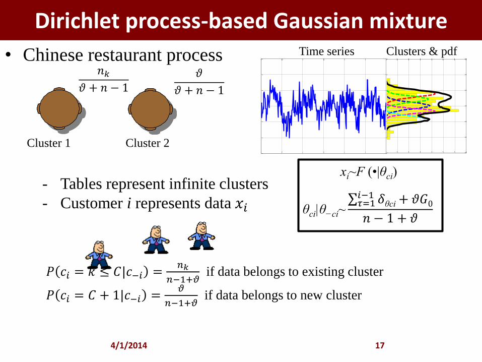
Dirichlet process-based Gaussian mixture
• Chinese restaurant process
4/1/2014 17
• 𝑥𝑖 -data points • 𝜃𝑖- distribution parameter drawn from
unknown distribution G
Cluster 1 Cluster 2
- Tables represent infinite clusters
- Customer i represents data 𝑥𝑖
𝑃 𝑐𝑖 = 𝑘 ≤ 𝐶|𝑐−𝑖 =𝑛𝑘
𝑛−1+𝜗 if data belongs to existing cluster
𝑃 𝑐𝑖 = 𝐶 + 1|𝑐−𝑖 =𝜗
𝑛−1+𝜗 if data belongs to new cluster
𝜗
𝜗 + 𝑛 − 1
𝑛𝑘𝜗 + 𝑛 − 1
0 50 100 150 200 250 300-15
-10
-5
0
5
10
15
Am
plit
ud
e
Time Index
-15
-10
-5
0
5
10
15
0
0.02
0.04
0.06
0.08
0.1
0.12
0.14
Time series Clusters & pdf
xi~F (•|θci)
θci|θ−ci~ 𝛿θci+ 𝜗𝐺0𝑖−1𝜏=1
𝑛 − 1 + 𝜗
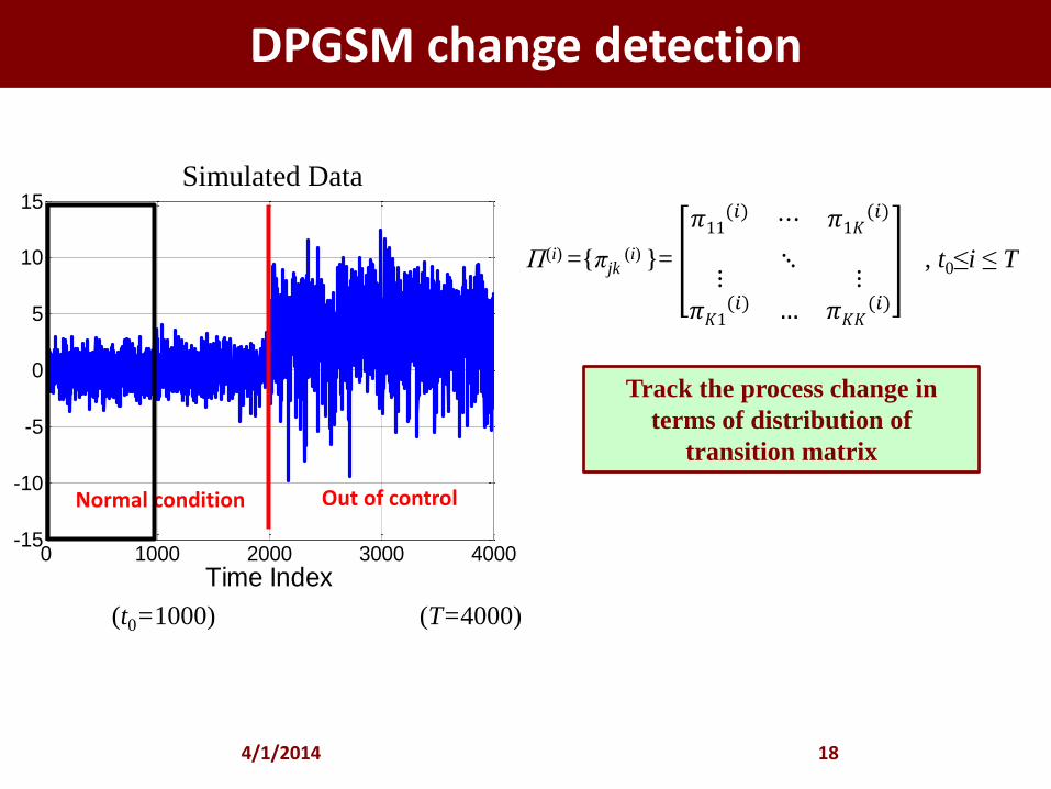
DPGSM change detection
4/1/2014 18
0 1000 2000 3000 4000-15
-10
-5
0
5
10
15
Am
plit
ud
e
Time Index
Simulated Data
Normal condition Out of control
(t0=1000)
𝜋11(𝑖) ⋯ 𝜋1𝐾
(𝑖)
⋮⋱
⋮𝜋𝐾1(𝑖) … 𝜋𝐾𝐾
(𝑖)
П(i) ={πjk (i) }=
(T=4000)
, t0≤i ≤ T
Track the process change in
terms of distribution of
transition matrix
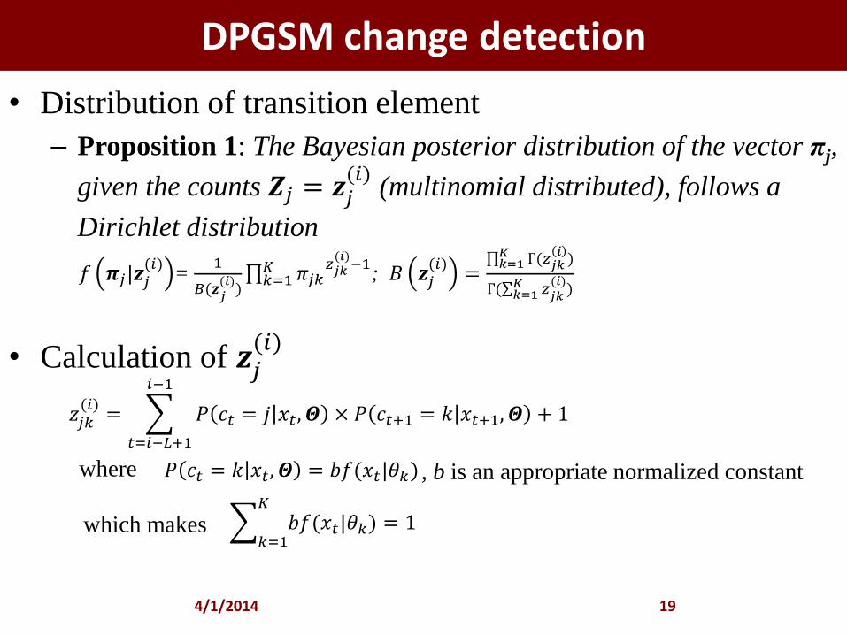
DPGSM change detection
• Distribution of transition element
– Proposition 1: The Bayesian posterior distribution of the vector πj,
given the counts 𝒁𝑗 = 𝒛𝑗(𝑖)
(multinomial distributed), follows a
Dirichlet distribution
• Calculation of 𝒛𝑗(𝑖)
4/1/2014 19
𝒛𝑗(𝑡)= {𝑧𝑗1
𝑡, … 𝑧𝑗𝑘
𝑡, … , 𝑧𝑗𝐾
(𝑡)}
𝑃 𝑐𝑡 = 𝑘 𝑥𝑡, 𝜣 = 𝑏𝑓(𝑥𝑡|𝜃𝑘) where
𝑏𝑓(𝑥𝑡|𝜃𝑘)𝐾
𝑘=1= 1
, b is an appropriate normalized constant
which makes
𝑓 𝝅𝑗|𝒛𝑗(𝑖)
= 1
𝐵(𝒛𝑗(𝑖)) 𝜋𝑗𝑘
𝑧𝑗𝑘(𝑖)−1𝐾
𝑘=1 ; 𝐵 𝒛𝑗(𝑖)= Г(𝑧𝑗𝑘
𝑖)𝐾
𝑘=1
Г( 𝑧𝑗𝑘(𝑖)𝐾
𝑘=1 )
𝑧𝑗𝑘(𝑖)= 𝑃 𝑐𝑡 = 𝑗 𝑥𝑡, 𝜣 × 𝑃 𝑐𝑡+1 = 𝑘 𝑥𝑡+1, 𝜣 + 1
𝑖−1
𝑡=𝑖−𝐿+1
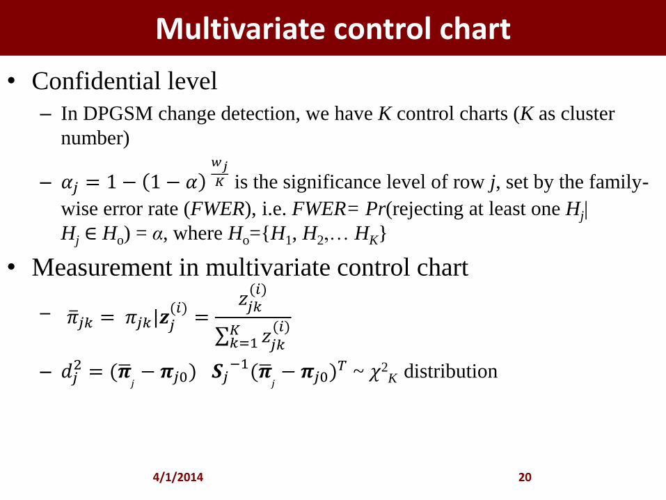
Multivariate control chart
• Confidential level
– In DPGSM change detection, we have K control charts (K as cluster
number)
– 𝛼𝑗 = 1 − 1 − 𝛼 𝑤𝑗
𝐾 is the significance level of row j, set by the family-
wise error rate (FWER), i.e. FWER= Pr(rejecting at least one Hj|
Hj ∈ Ho) = α, where Ho={H1, H2,… HK}
• Measurement in multivariate control chart
–
– 𝑑𝑗2 = (𝝅
𝑗− 𝝅𝑗0) 𝑺𝑗
−1(𝝅 𝑗− 𝝅𝑗0)
𝑇 ~ 𝜒2K distribution
4/1/2014 20
𝜋 𝑗𝑘 = 𝜋𝑗𝑘|𝒛𝑗(𝑖)=𝑧𝑗𝑘(𝑖)
𝑧𝑗𝑘(𝑖)𝐾
𝑘=1
0 1000 2000 3000 4000 5000 6000
-20
-15
-10
-5
0
5
10
15
20
Am
plit
ud
e
Time Index
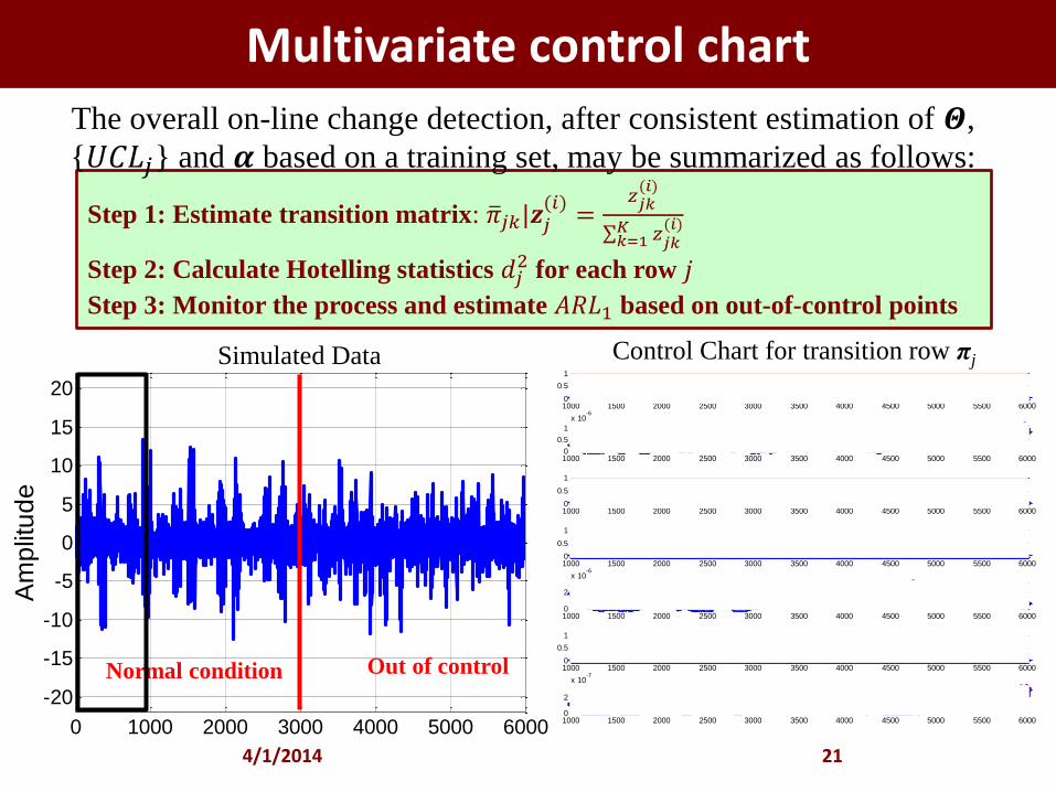
Multivariate control chart
4/1/2014 21
Control Chart for transition row πj Simulated Data
Normal condition Out of control
1000 1500 2000 2500 3000 3500 4000 4500 5000 5500 60000
0.5
1
1000 1500 2000 2500 3000 3500 4000 4500 5000 5500 60000
0.5
1
x 10-6
1000 1500 2000 2500 3000 3500 4000 4500 5000 5500 60000
0.5
1
1000 1500 2000 2500 3000 3500 4000 4500 5000 5500 60000
0.5
1
1000 1500 2000 2500 3000 3500 4000 4500 5000 5500 60000
2
x 10-6
1000 1500 2000 2500 3000 3500 4000 4500 5000 5500 60000
0.5
1
1000 1500 2000 2500 3000 3500 4000 4500 5000 5500 60000
2
x 10-7
Step 1: Estimate transition matrix: 𝜋 𝑗𝑘|𝒛𝑗(𝑖)=
𝑧𝑗𝑘(𝑖)
𝑧𝑗𝑘(𝑖)𝐾
𝑘=1
Step 2: Calculate Hotelling statistics 𝑑𝑗2 for each row 𝑗
Step 3: Monitor the process and estimate 𝐴𝑅𝐿1 based on out-of-control points
The overall on-line change detection, after consistent estimation of 𝜣,
{𝑈𝐶𝐿𝑗} and 𝜶 based on a training set, may be summarized as follows:
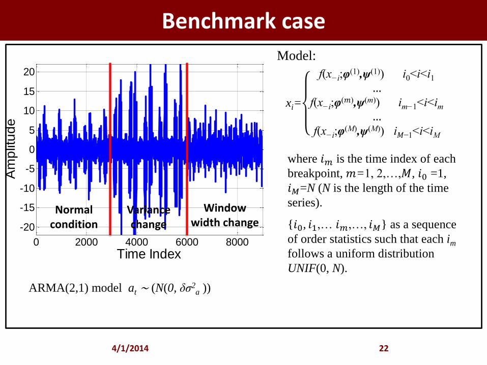
Benchmark case
4/1/2014 22
ARMA(2,1) model at ∼ (N(0, δσ2a ))
0 2000 4000 6000 8000
-20
-15
-10
-5
0
5
10
15
20
Am
plit
ud
e
Time Index
Variance change
Window width change
Normal condition
Model:
where 𝑖𝑚 is the time index of each
breakpoint, 𝑚=1, 2,…,𝑀, 𝑖0 =1,
𝑖𝑀=N (N is the length of the time
series).
xi=
f(x−i;φ(1),ψ(1)) i0<i<i1
…f(x−i;φ
(𝑚),ψ(m)) im−1<i<im
…f(x−i;φ
(M),ψ(M)) i𝑀−1<i<iM
{𝑖0, 𝑖1,… 𝑖𝑚,…, 𝑖𝑀} as a sequence
of order statistics such that each im
follows a uniform distribution
UNIF(0, N).
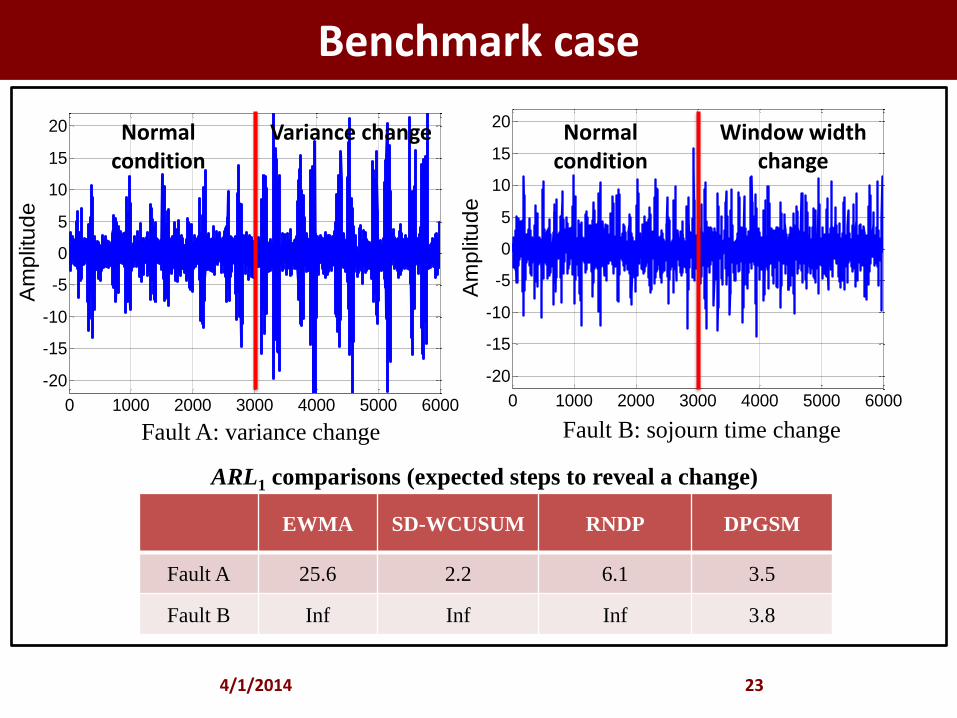
Benchmark case
4/1/2014 23
0 1000 2000 3000 4000 5000 6000
-20
-15
-10
-5
0
5
10
15
20
Am
plit
ud
e
Time Index
EWMA SD-WCUSUM RNDP DPGSM
Fault A 25.6 2.2 6.1 3.5
Fault B Inf Inf Inf 3.8
Variance change Normal condition
Fault A: variance change Fault B: sojourn time change
0 1000 2000 3000 4000 5000 6000
-20
-15
-10
-5
0
5
10
15
20
Am
plit
ud
e
Time Index
Window width change
Normal condition
ARL1 comparisons (expected steps to reveal a change)
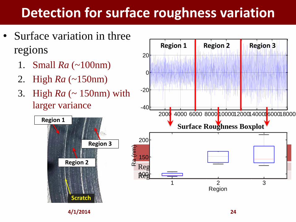
Detection for surface roughness variation
• Surface variation in three
regions
1. Small Ra (~100nm)
2. High Ra (~150nm)
3. High Ra (~ 150nm) with
larger variance
4/1/2014 24
2000 4000 6000 80001000012000140001600018000-40
-20
0
20
Expected delay of detection (ms)
Region 1 Region 2 Region 3
DPGSM achieves consistently low
ARL1 for detecting incipient
surface quality variation within
nano level
EWMA SD-
WCUSUM DPGSM
Region 1-2 10.4 1.5 0.5
Region 2-3 21.4 0.4 0.4
Region 2
Region 1
Region 3
Scratch
1 2 3
100
150
200R
a (
nm
)
Region
Surface Roughness Boxplot
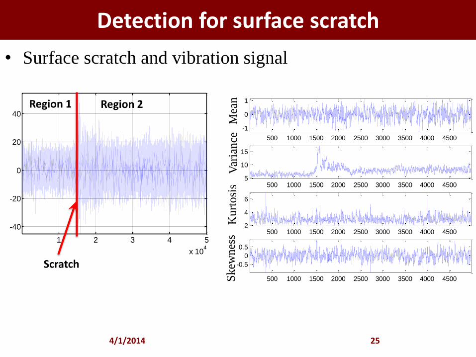
Detection for surface scratch
• Surface scratch and vibration signal
4/1/2014 25
1 2 3 4 5
x 104
-40
-20
0
20
40
500 1000 1500 2000 2500 3000 3500 4000 4500
-1
0
1
500 1000 1500 2000 2500 3000 3500 4000 45005
10
15
500 1000 1500 2000 2500 3000 3500 4000 45002
4
6
500 1000 1500 2000 2500 3000 3500 4000 4500
-0.5
0
0.5
Mea
n
Var
iance
K
urt
osi
s S
kew
nes
s
Scratch
Region 1 Region 2
0 200 400 600 800 1000 12004
6
8
10
12
14
16
18
Time index
Ou
tpu
t
prediction
observation
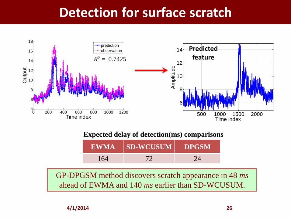
Detection for surface scratch
4/1/2014 26
R2 = 0.7425
500 1000 1500 2000
6
8
10
12
14
Am
plit
ud
e
Time Index
Predicted feature
Expected delay of detection(ms) comparisons
EWMA SD-WCUSUM DPGSM
164 72 24
GP-DPGSM method discovers scratch appearance in 48 ms
ahead of EWMA and 140 ms earlier than SD-WCUSUM.

Change detection of surface deterioration
• Chemical Mechanical Planarization
(CMP) process experiment
– Lapped coppers (Ra 10nm~15nm)
were polished on Buehler in 3
minutes of each interval
– Platen speed 250 RPM, head speed
60 RPM and download force 4 lbs
4/1/2014 27
Buehler (model Automet® 250)
with 3-axis accelerometer
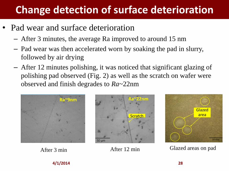
Change detection of surface deterioration
• Pad wear and surface deterioration
– After 3 minutes, the average Ra improved to around 15 nm
– Pad wear was then accelerated worn by soaking the pad in slurry,
followed by air drying
– After 12 minutes polishing, it was noticed that significant glazing of
polishing pad observed (Fig. 2) as well as the scratch on wafer were
observed and finish degrades to Ra~22nm
4/1/2014 28
After 3 min After 12 min Glazed areas on pad
Ra~9nm Ra~22nm
Scratch
Glazed area
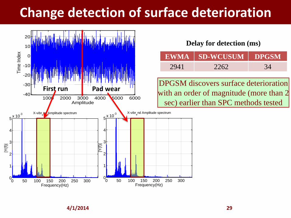
Change detection of surface deterioration
4/1/2014 29
1000 2000 3000 4000 5000 6000-40
-30
-20
-10
0
10
20
Tim
e I
nd
ex
Amplitude
First run Pad wear
0 50 100 150 200 250 3000
1
2
3
4
5x 10
-3 X-vibrend Amplitude spectrum
Frequency(Hz)
|Y(f
)|
0 50 100 150 200 250 3000
1
2
3
4
5x 10
-3 X-vibrend Amplitude spectrum
Frequency(Hz)
|Y(f
)|
EWMA SD-WCUSUM DPGSM
2941 2262 34
Delay for detection (ms)
DPGSM discovers surface deterioration
with an order of magnitude (more than 2
sec) earlier than SPC methods tested
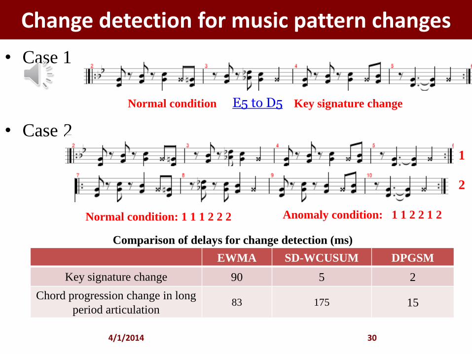
Change detection for music pattern changes
• Case 1
• Case 2
4/1/2014 30
Normal condition Key signature change
Normal condition: 1 1 1 2 2 2 Anomaly condition: 1 1 2 2 1 2
1
2
EWMA SD-WCUSUM DPGSM
Key signature change 90 5 2
Chord progression change in long
period articulation 83 175 15
E5 to D5
Comparison of delays for change detection (ms)

Change detection in Ragas
4/1/2014 32
General types of Raga music
Change detection 1: Sequence
change with ascending and
descending scales
Change detection 2: Scale
change with missing notes
Subtle changes in intermittent music signals, namely scores sequence
change and music scale change, are considered.
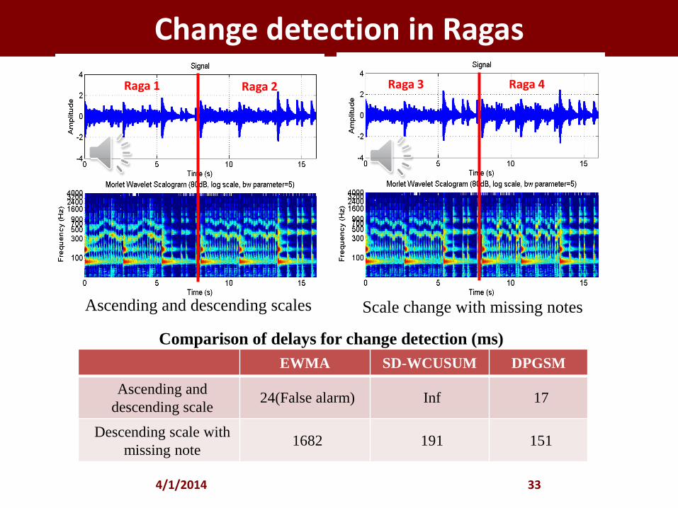
Change detection in Ragas
4/1/2014 33
Raga 3 Raga 2 Raga 4 Raga 1
EWMA SD-WCUSUM DPGSM
Ascending and
descending scale 24(False alarm) Inf 17
Descending scale with
missing note 1682 191 151
Ascending and descending scales Scale change with missing notes
Comparison of delays for change detection (ms)
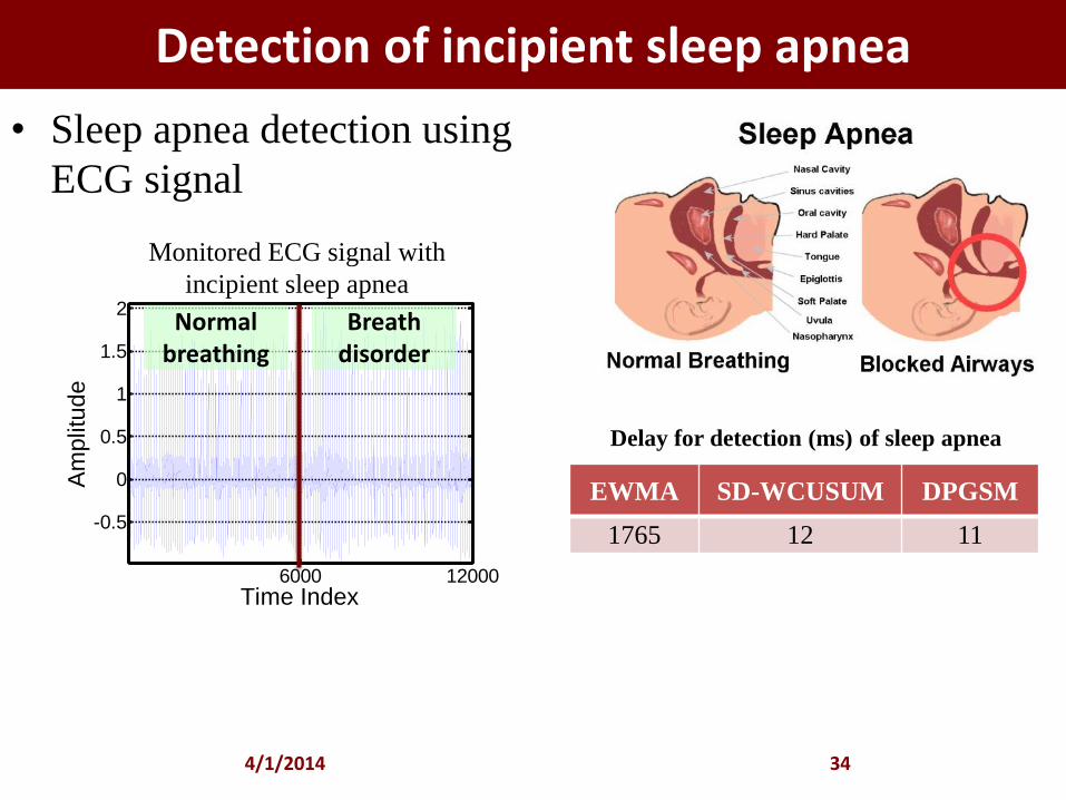
Detection of incipient sleep apnea
• Sleep apnea detection using
ECG signal
4/1/2014 34
6000 12000
-0.5
0
0.5
1
1.5
2
Am
plit
ud
e
Time Index
EWMA SD-WCUSUM DPGSM
1765 12 11
Delay for detection (ms) of sleep apnea
Monitored ECG signal with
incipient sleep apnea
Normal breathing
Breath disorder

Conclusions
• We represent nonlinear nonstationary (intermittency) signal within
precision machining processes as a stochastic mixture of Gaussian
clusters with Markov transition matrix
• Intermittent changes in surface uniformity are efficiently identified by
DPGSM, and it could detect surface damage (scratch) almost an order
of magnitude earlier compared to existing change detection methods
(EWMA and SD-WCUSUM)
4/1/2014 35
Further studies
• Parameters selection
– Selection of window length 𝑳 is crucial to derive consistent estimates of
the transition matrix elements
– Selection of the concentration parameter 𝝑 of Dirichlet process to
ensure generation of proper Gaussian mixtures
• The transition process may be more closely approximated using a
semi-Markov formulation and the representation needs to be
modified to better capture the underlying dynamics
4/1/2014 36