4/21/2008

20 Curved

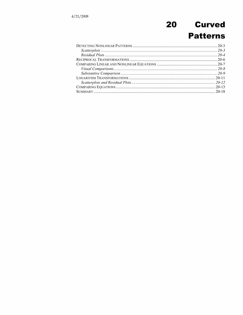
Patterns DETECTING NONLINEAR PATTERNS ..................................................................................... 20-3

Scatterplots ..................................................................................................................... 20-3 Residual Plots ................................................................................................................. 20-4

RECIPROCAL TRANSFORMATIONS ........................................................................................ 20-6 COMPARING LINEAR AND NONLINEAR EQUATIONS ............................................................. 20-7

Visual Comparisons ........................................................................................................ 20-8 Substantive Comparison ................................................................................................. 20-9

LOGARITHM TRANSFORMATIONS ....................................................................................... 20-11 Scatterplots and Residual Plots .................................................................................... 20-12

COMPARING EQUATIONS .................................................................................................... 20-13 SUMMARY .......................................................................................................................... 20-18

4/21/2008 20 Curves

20-2

Figure 20-1. Average retail price of regular unleaded gasoline in the US, in dollars per gallon.

An increase in the price of gasoline is a painful reminder of the laws of supply and demand. The first big increase in domestic prices struck in 1973-1974 when the Organization of Petroleum Exporting Countries (OPEC) set production quotas. Gasoline prices had been nearly constant for so long that no one kept track of prices before then. These data start in 1975, shortly before the surge that began in 1979. After selling for 60 to 70 cents a gallon during the 1970’s, the average price soared above $1.40 per gallon in 1981.

Congress noticed the importance of energy prices as well. The legislative response included the Energy Policy and Conservation Act of 1975. This act established corporate average fuel economy (CAFE) standards for passenger vehicles sold in the US. The current standard for cars is 27.5 mpg (light trucks need to average 20.7 mpg). Until recently, fuel efficiency hadn’t received much legislative attention since then.

More recent price increases have renewed interest in improving the efficiency of cars. One way to improve mileage is to reduce the weight of the car. Lighter materials, however, cost more than heavier materials of comparable strength. Aluminum and composites are more expensive than steel.

Companies want evidence of the benefit before they sink money into lightweight materials. What sort of improvements in mileage should a manufacturer expect from reducing the weight of a car by, say, 200 pounds? That’s not much for one car, but the costs and benefits add up when you make millions.

To answer this question, we’ll use a regression model. Unlike models in Chapter 19, this model has to capture a pattern that bends.

2005 Ford Escape MPG 31 City / 36 Hwy

2005 Mercedes G55 MPG 12 City / 14 Hwy

4/21/2008 20 Curves

20-3

Detecting Nonlinear Patterns Linear patterns are a good place to begin when modeling dependence, but they don’t work in every situation. There are two ways to recognize problems with linear equations: one you should do before you look at the data and the other you judge from a plot.

Before you start working with data and plots, ask yourself the question, “Why should changes in x come with constant changes in y?” Linear association means that a change in x on average is associated with a constant change in y. For example, a linear equation nicely describes the association between weight and price of small diamonds in Chapter 19. Each increase in weight by one tenth of a carat increases the estimated price by $267, regardless of the size of the diamond. A quick visit to a jeweler should convince you, however, that the difference in price between ½ carat diamonds and 1-carat diamonds is smaller than the gap between 1.5 and 2-carat diamonds. As diamonds get larger, they become scarcer and increments in size command ever larger increments in price.

For cars, do you expect the effect of weight on mileage to be the same for cars of all sizes? Does trimming 200 pounds from a big SUV have the same effect on mileage as trimming 200 pounds from a small compact? If we model the relationship between mileage (y) and weight (x) using a line, then our answer is “yes.” A fitted line

€

ˆ y = b0 + b1 x has one slope, regardless of x. Before we accept this claim, we need to look at data.

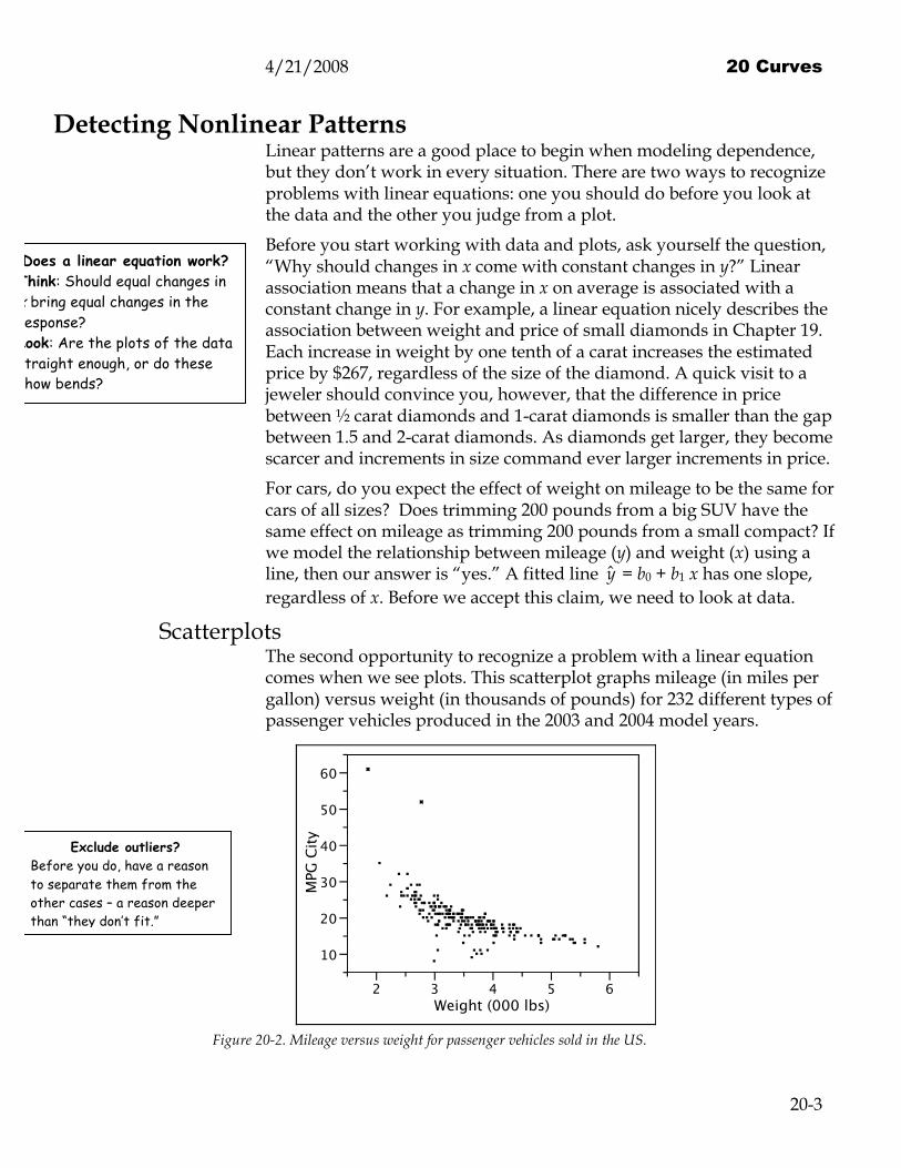
Scatterplots The second opportunity to recognize a problem with a linear equation comes when we see plots. This scatterplot graphs mileage (in miles per gallon) versus weight (in thousands of pounds) for 232 different types of passenger vehicles produced in the 2003 and 2004 model years.

10

20

30

40

50

60

MPG

City

2 3 4 5 6Weight (000 lbs)

Figure 20-2. Mileage versus weight for passenger vehicles sold in the US.

Does a linear equation work? Think: Should equal changes in x bring equal changes in the response? Look: Are the plots of the data straight enough, or do these show bends?

Exclude outliers? Before you do, have a reason to separate them from the other cases – a reason deeper than “they don’t fit.”

4/21/2008 20 Curves

20-4

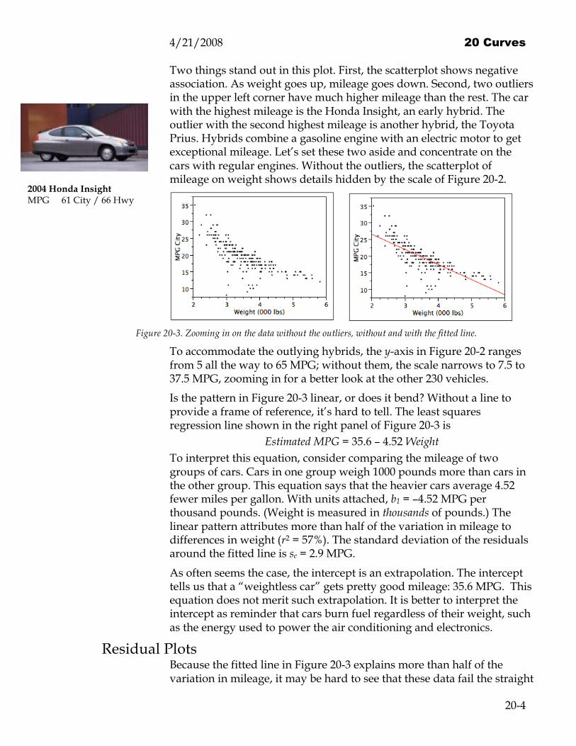
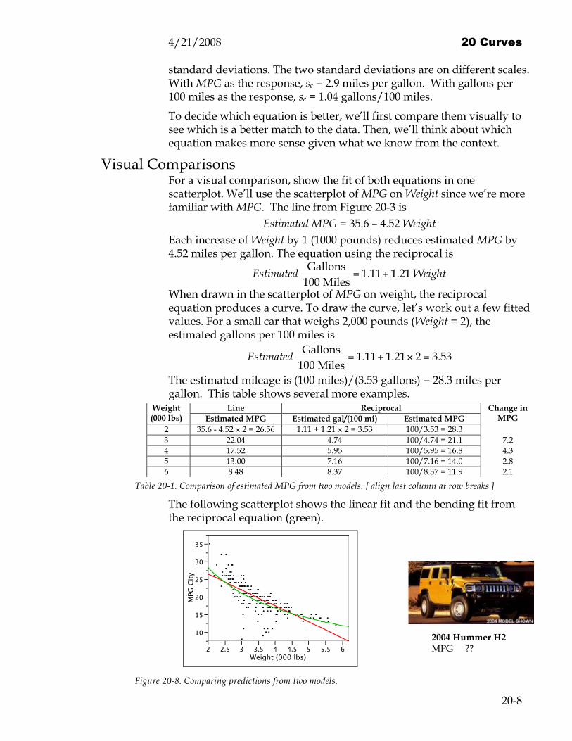
Two things stand out in this plot. First, the scatterplot shows negative association. As weight goes up, mileage goes down. Second, two outliers in the upper left corner have much higher mileage than the rest. The car with the highest mileage is the Honda Insight, an early hybrid. The outlier with the second highest mileage is another hybrid, the Toyota Prius. Hybrids combine a gasoline engine with an electric motor to get exceptional mileage. Let’s set these two aside and concentrate on the cars with regular engines. Without the outliers, the scatterplot of mileage on weight shows details hidden by the scale of Figure 20-2.

Figure 20-3. Zooming in on the data without the outliers, without and with the fitted line.

To accommodate the outlying hybrids, the y-axis in Figure 20-2 ranges from 5 all the way to 65 MPG; without them, the scale narrows to 7.5 to 37.5 MPG, zooming in for a better look at the other 230 vehicles.

Is the pattern in Figure 20-3 linear, or does it bend? Without a line to provide a frame of reference, it’s hard to tell. The least squares regression line shown in the right panel of Figure 20-3 is

Estimated MPG = 35.6 – 4.52 Weight To interpret this equation, consider comparing the mileage of two groups of cars. Cars in one group weigh 1000 pounds more than cars in the other group. This equation says that the heavier cars average 4.52 fewer miles per gallon. With units attached, b1 = –4.52 MPG per thousand pounds. (Weight is measured in thousands of pounds.) The linear pattern attributes more than half of the variation in mileage to differences in weight (r2 = 57%). The standard deviation of the residuals around the fitted line is se = 2.9 MPG.

As often seems the case, the intercept is an extrapolation. The intercept tells us that a “weightless car” gets pretty good mileage: 35.6 MPG. This equation does not merit such extrapolation. It is better to interpret the intercept as reminder that cars burn fuel regardless of their weight, such as the energy used to power the air conditioning and electronics.

Residual Plots Because the fitted line in Figure 20-3 explains more than half of the variation in mileage, it may be hard to see that these data fail the straight

2004 Honda Insight MPG 61 City / 66 Hwy

4/21/2008 20 Curves

20-5

enough condition. If you look closely at Figure 20-3, you can see that the line passes below most of the points that represent light cars, above most in the middle, and again too low at the right for large cars.

The lack of fit becomes more apparent in the residual plot. After removing the linear trend, the curving pattern is more evident.

-15

-10

-5

0

5

10

Resi

dual

2 3 4 5 6Weight (000 lbs)

Figure 20-4. Residual plot with sketched-in bending curve.

The sketched curve suggests a bending pattern. The residuals are generally positive on the left (light cars), negative in the middle, and positive at the right (heavy cars). The plot seems to grin at us. This curvature also appears in scatterplot of MPG on Weight in Figure 20-3, but the residual plot makes it more apparent. Once you see the pattern in the residual plot, you can usually find it in the original scatterplot of y on x as well.

To confirm the presence of a pattern in the residuals, use the visual test for simplicity (Chapter 6). To make a comparison, build another scatterplot that scrambles the weights so that each residual gets matched to a randomly chosen weight. If there’s no pattern, then it should not matter which weight goes with which residual. The following figure shows two such scatterplots.

-15

-10

-5

0

5

10

Resi

dual

s M

PG C

ity

2 3 4 5 6Scrambled Weights

-15

-10

-5

0

5

10

Resi

dual

s M

PG C

ity

2 3 4 5 6Scrambled Weights

Figure 20-5. Checking for simple residuals.

The residual plot in Figure 20-4 is distinct from these. The scales are the same, but the content is visually rather different. That means there’s a pattern in the residuals. Because the association in the data is not straight enough, we need to find a nonlinear equation to represent the dependence.

4/21/2008 20 Curves

20-6

Reciprocal Transformations Transformations expand the scope of regression modeling and allow us to describe patterns that curve. A transformation is a function that is applied to a column of data. By applying a transformation to either x or y (or both), we can build nonlinear equations that describe the relationship better than a linear equation. We concentrate on two transformations that are most useful in business applications: reciprocals and logarithms. The reciprocal transformation converts the data di in the ith row of the data table into its reciprocal 1/di. Similarly, the log transformation converts di into log di. We can apply transformations to the explanatory variable or to the response.

By connecting reciprocals and logarithms to the substance of problems, we can interpret nonlinear equations that use these transformations. Reciprocals work well when dealing with rates or ratios, and logs connect patterns to the underlying economics and percentages. Other transformations often produce an equation that is beyond interpretation. If you cannot interpret an equation, how are you going to use it?

A reciprocal transformation captures the bending pattern between MPG and Weight. We will replace MPG by the number of gallons that it takes to go 100 miles. This transformation is 100 × 1/MPG. Europeans measure fuel efficiency on a similar scale in liters per 100 kilometers. The reciprocal is interpretable because MPG is a ratio, miles per gallon. The reciprocal transformation measures gallons per mile. (Multiplying by 100 gives a more useful range of values.) This scatterplot graphs fuel consumption in gallons per 100 miles versus weight.

23456789

10111213

Gallo

ns/(

100

mile

s)

2 2.5 3 3.5 4 4.5 5 5.5 6Weight (000 lbs)

Figure 20-6. Transforming to a simpler pattern.

The scatterplot includes the least squares line. The association is positive because the response measures fuel consumption rather than fuel efficiency. Heavier cars consume more gas, so the slope is positive. The pattern looks linear but for a scattering of outliers that are less obvious in Figure 20-3. Any guess which cars have very high fuel consumption for their weights?

1/d1

1/d2

1/d3

1/d4

…

d1

d2

d3

d4

…

log d1

log d2

log d3

log d4

…

1/d

log d

How’d you know to try that? (1) Experience (2) Tried several others (3) Context. That’s how they measure mileage in Europe.

4/21/2008 20 Curves

20-7

The previous outliers are fuel-efficient hybrids; these gas-guzzling outliers are at the other end of the scale. The outliers are even more apparent in the following residual plot.

-2-10123456789

Resi

dual

2 2.5 3 3.5 4 4.5 5 5.5 6Weight (000 lbs)

Figure 20-7. Residuals from the regression using a reciprocal of y.

The outliers are exotic sports cars: a Ferrari, a Lamborghini, a Masarati, and an Aston Martin. The Ferrari Enzo has the largest positive residual; it needs 8 more gallons to go 100 miles than typical cars of its weight. It also packs 660 horsepower. No matter how light you make the car, an engine that generates that kind of power burns a lot of gas.

By transforming miles per gallon into gallons per 100 miles, we’ve constructed an equation that appears more linear than the initial fit. The equation for the least squares line in Figure 20-7 is

Estimated Gallons/100 miles = 1.11 + 1.21 Weight

In spite of these outliers, the relationship appears linear.

The use of a transformation also changes the interpretation of the slope and intercept. To interpret b0 and b1 in this equation, think again about two groups of cars. Cars in one group weigh 1,000 pounds more than those in the other. The slope in this equation means that, on average, the heavier cars use 1.21 more gallons to drive 100 miles. The intercept naively speaks of weightless cars, but in terms of gallons per 100 miles. The intercept remains a big extrapolation if we think of it as a prediction. It’s more interesting if we interpret it as the fuel burned regardless of the weight. These cars use about 1.1 gallons when driving 100 miles to run air conditioning and other conveniences, regardless of the weight.

Comparing Linear and Nonlinear Equations Which equation is better?

It is tempting to choose the fit with the larger r2. The r2 of the initial linear equation is higher, 57% to 41%. Before you conclude this is a meaningful comparison, notice that the equations use different responses. Explaining 57% of the variation in mileage is not comparable to explaining 41% of the variation in fuel consumption. That’s not a meaningful comparison. Only compare r2 between regression equations that use the same response. The same goes for comparisons of the residual

2003 Ferrari Enzo MPG 8 City / 12 Hwy

tip

4/21/2008 20 Curves

20-8

standard deviations. The two standard deviations are on different scales. With MPG as the response, se = 2.9 miles per gallon. With gallons per 100 miles as the response, se = 1.04 gallons/100 miles.

To decide which equation is better, we’ll first compare them visually to see which is a better match to the data. Then, we’ll think about which equation makes more sense given what we know from the context.

Visual Comparisons For a visual comparison, show the fit of both equations in one scatterplot. We’ll use the scatterplot of MPG on Weight since we’re more familiar with MPG. The line from Figure 20-3 is

Estimated MPG = 35.6 – 4.52 Weight Each increase of Weight by 1 (1000 pounds) reduces estimated MPG by 4.52 miles per gallon. The equation using the reciprocal is

€

Estimated Gallons

100 Miles= 1.11+ 1.21 Weight

When drawn in the scatterplot of MPG on weight, the reciprocal equation produces a curve. To draw the curve, let’s work out a few fitted values. For a small car that weighs 2,000 pounds (Weight = 2), the estimated gallons per 100 miles is

€

Estimated Gallons

100 Miles= 1.11 + 1.21× 2 = 3.53

The estimated mileage is (100 miles)/(3.53 gallons) = 28.3 miles per gallon. This table shows several more examples.

Table 20-1. Comparison of estimated MPG from two models. [ align last column at row breaks ]

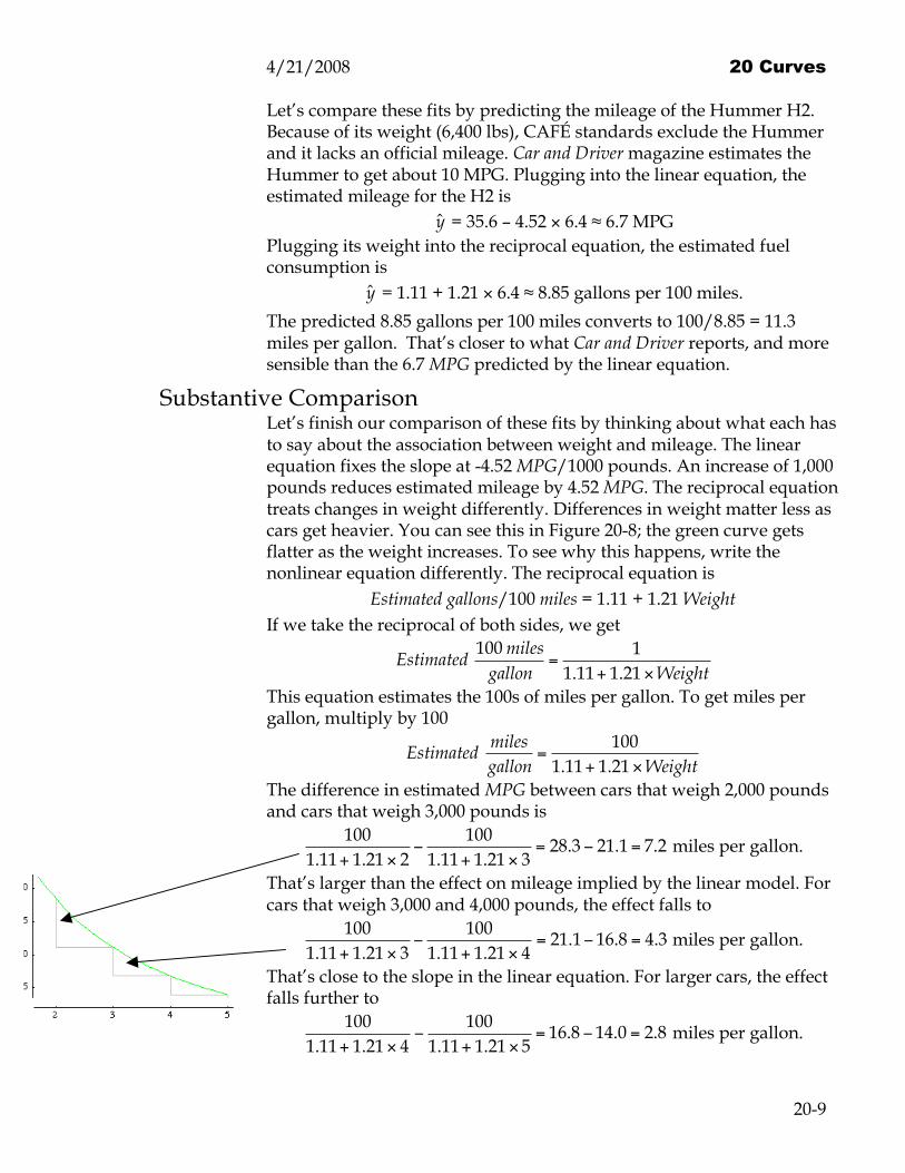
The following scatterplot shows the linear fit and the bending fit from the reciprocal equation (green).

10

15

20

25

30

35

MPG

City

2 2.5 3 3.5 4 4.5 5 5.5 6Weight (000 lbs)

Figure 20-8. Comparing predictions from two models.

Line Reciprocal Weight (000 lbs) Estimated MPG Estimated gal/(100 mi) Estimated MPG

Change in MPG

2 35.6 - 4.52 × 2 = 26.56 1.11 + 1.21 × 2 = 3.53 100/3.53 = 28.3 3 22.04 4.74 100/4.74 = 21.1 7.2 4 17.52 5.95 100/5.95 = 16.8 4.3 5 13.00 7.16 100/7.16 = 14.0 2.8 6 8.48 8.37 100/8.37 = 11.9 2.1

2004 Hummer H2 MPG ??

4/21/2008 20 Curves

20-9

Let’s compare these fits by predicting the mileage of the Hummer H2. Because of its weight (6,400 lbs), CAFÉ standards exclude the Hummer and it lacks an official mileage. Car and Driver magazine estimates the Hummer to get about 10 MPG. Plugging into the linear equation, the estimated mileage for the H2 is

€

ˆ y = 35.6 – 4.52 × 6.4 ≈ 6.7 MPG Plugging its weight into the reciprocal equation, the estimated fuel consumption is

€

ˆ y = 1.11 + 1.21 × 6.4 ≈ 8.85 gallons per 100 miles.

The predicted 8.85 gallons per 100 miles converts to 100/8.85 = 11.3 miles per gallon. That’s closer to what Car and Driver reports, and more sensible than the 6.7 MPG predicted by the linear equation.

Substantive Comparison Let’s finish our comparison of these fits by thinking about what each has to say about the association between weight and mileage. The linear equation fixes the slope at -4.52 MPG/1000 pounds. An increase of 1,000 pounds reduces estimated mileage by 4.52 MPG. The reciprocal equation treats changes in weight differently. Differences in weight matter less as cars get heavier. You can see this in Figure 20-8; the green curve gets flatter as the weight increases. To see why this happens, write the nonlinear equation differently. The reciprocal equation is

Estimated gallons/100 miles = 1.11 + 1.21 Weight If we take the reciprocal of both sides, we get

€

Estimated100 miles

gallon=

11.11+ 1.21 ×Weight

This equation estimates the 100s of miles per gallon. To get miles per gallon, multiply by 100

€

Estimatedmilesgallon

=100

1.11 + 1.21 ×Weight

The difference in estimated MPG between cars that weigh 2,000 pounds and cars that weigh 3,000 pounds is

€

1001.11+ 1.21 × 2

−100

1.11+ 1.21 × 3= 28.3 − 21.1 = 7.2 miles per gallon.

That’s larger than the effect on mileage implied by the linear model. For cars that weigh 3,000 and 4,000 pounds, the effect falls to

€

1001.11+ 1.21 × 3

−100

1.11+ 1.21 × 4= 21.1− 16.8 = 4.3 miles per gallon.

That’s close to the slope in the linear equation. For larger cars, the effect falls further to

€

1001.11+ 1.21 × 4

−100

1.11+ 1.21 × 5= 16.8 − 14.0 = 2.8 miles per gallon.

4/21/2008 20 Curves

20-10

The curve is steeper for small cars and flatter for large cars: differences in weight matter more for small cars. That seems to make more sense than a constant decrease. After all, mileage can only go down to zero.

Do these differences matter? They do if you are an automotive engineer charged with improving mileage. Suppose that engineers estimate the benefits of reducing weight by 200 pounds using the linear equation. They would conclude that reducing weight brings an average improvement of 0.2 × 4.52 ≈ 0.9 MPG, or about one more mile per gallon. The reciprocal equation tells a different story. Shaving 200 pounds from a 3,000-pound car improves the mileage by 33% more:

€

1001.11+ 1.21 × 2.8

−100

1.11 + 1.21 × 3= 22.2 − 21.1 = 1.2 miles per gallon.

For a 5,000-pound SUV, however, the improvement is much less,

€

1001.11+ 1.21 × 4.8

−100

1.11 + 1.21 × 5= 14.5 − 14.0 = 0.5 miles per gallon.

The reciprocal shows the engineers where to focus their efforts to make the most difference. It might be easy to trim 200 pounds from a heavy SUV, but it’s not going to have much effect on mileage.

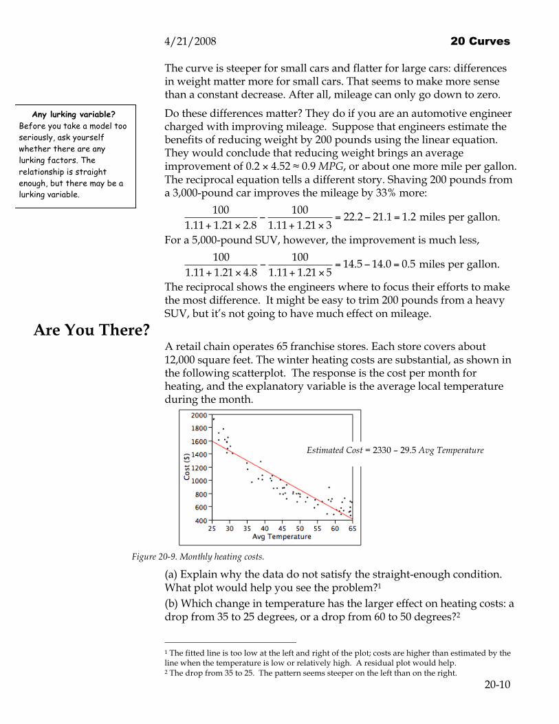
Are You There? A retail chain operates 65 franchise stores. Each store covers about 12,000 square feet. The winter heating costs are substantial, as shown in the following scatterplot. The response is the cost per month for heating, and the explanatory variable is the average local temperature during the month.

Figure 20-9. Monthly heating costs.

(a) Explain why the data do not satisfy the straight-enough condition. What plot would help you see the problem?1 (b) Which change in temperature has the larger effect on heating costs: a drop from 35 to 25 degrees, or a drop from 60 to 50 degrees?2

1 The fitted line is too low at the left and right of the plot; costs are higher than estimated by the line when the temperature is low or relatively high. A residual plot would help. 2 The drop from 35 to 25. The pattern seems steeper on the left than on the right.

Estimated Cost = 2330 – 29.5 Avg Temperature

Any lurking variable? Before you take a model too seriously, ask yourself whether there are any lurking factors. The relationship is straight enough, but there may be a lurking variable.

4/21/2008 20 Curves

20-11

(c) Sketch a bending pattern that captures the relationship between temperature and cost better than the fitted line.3

Logarithm Transformations How much should a retailer charge for merchandise? At a high price, each sale brings a large profit, but economics suggests that fewer items sell than at a lower price. Low prices generate more volume, but each sale brings less profit.

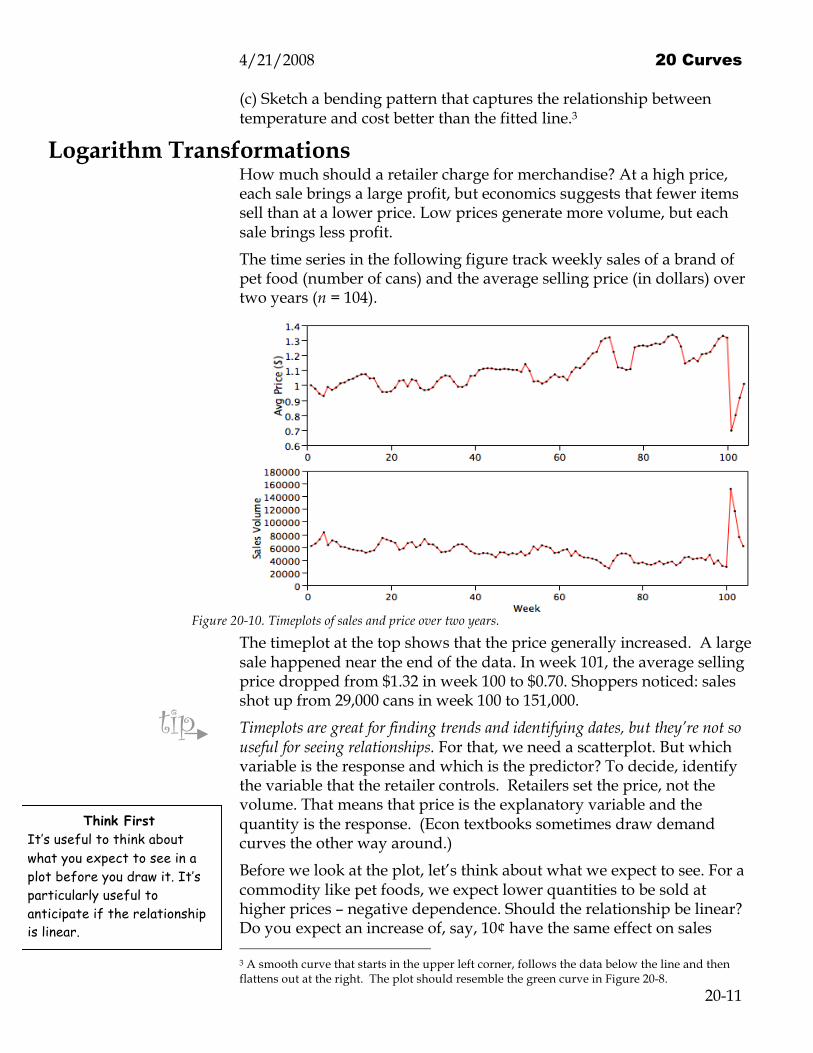
The time series in the following figure track weekly sales of a brand of pet food (number of cans) and the average selling price (in dollars) over two years (n = 104).

Figure 20-10. Timeplots of sales and price over two years.

The timeplot at the top shows that the price generally increased. A large sale happened near the end of the data. In week 101, the average selling price dropped from $1.32 in week 100 to $0.70. Shoppers noticed: sales shot up from 29,000 cans in week 100 to 151,000.

Timeplots are great for finding trends and identifying dates, but they’re not so useful for seeing relationships. For that, we need a scatterplot. But which variable is the response and which is the predictor? To decide, identify the variable that the retailer controls. Retailers set the price, not the volume. That means that price is the explanatory variable and the quantity is the response. (Econ textbooks sometimes draw demand curves the other way around.)

Before we look at the plot, let’s think about what we expect to see. For a commodity like pet foods, we expect lower quantities to be sold at higher prices – negative dependence. Should the relationship be linear? Do you expect an increase of, say, 10¢ have the same effect on sales 3 A smooth curve that starts in the upper left corner, follows the data below the line and then flattens out at the right. The plot should resemble the green curve in Figure 20-8.

Think First It’s useful to think about what you expect to see in a plot before you draw it. It’s particularly useful to anticipate if the relationship is linear.

tip

4/21/2008 20 Curves

20-12

when the price is $0.70 as when the price is $1.20? It does if the relationship is linear.

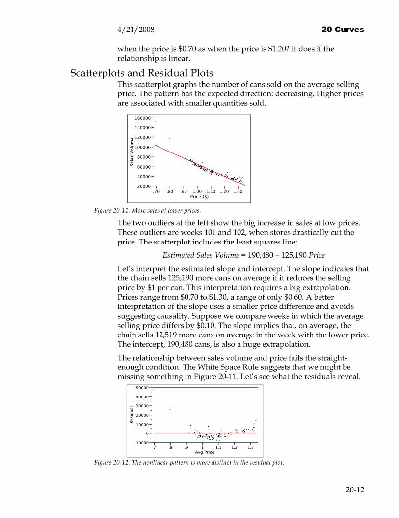
Scatterplots and Residual Plots This scatterplot graphs the number of cans sold on the average selling price. The pattern has the expected direction: decreasing. Higher prices are associated with smaller quantities sold.

20000

40000

60000

80000

100000

120000

140000

160000

Sale

s Vo

lum

e

.70 .80 .90 1.00 1.10 1.20 1.30Price ($)

Figure 20-11. More sales at lower prices.

The two outliers at the left show the big increase in sales at low prices. These outliers are weeks 101 and 102, when stores drastically cut the price. The scatterplot includes the least squares line:

Estimated Sales Volume = 190,480 – 125,190 Price

Let’s interpret the estimated slope and intercept. The slope indicates that the chain sells 125,190 more cans on average if it reduces the selling price by $1 per can. This interpretation requires a big extrapolation. Prices range from $0.70 to $1.30, a range of only $0.60. A better interpretation of the slope uses a smaller price difference and avoids suggesting causality. Suppose we compare weeks in which the average selling price differs by $0.10. The slope implies that, on average, the chain sells 12,519 more cans on average in the week with the lower price. The intercept, 190,480 cans, is also a huge extrapolation.

The relationship between sales volume and price fails the straight-enough condition. The White Space Rule suggests that we might be missing something in Figure 20-11. Let’s see what the residuals reveal.

-10000

0

10000

20000

30000

40000

50000

Resi

dual

.7 .8 .9 1 1.1 1.2 1.3Avg Price

Figure 20-12. The nonlinear pattern is more distinct in the residual plot.

4/21/2008 20 Curves

20-13

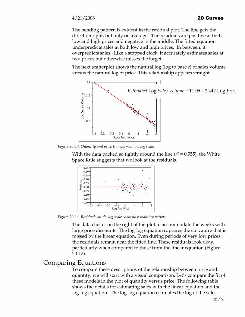
The bending pattern is evident in the residual plot. The line gets the direction right, but only on average. The residuals are positive at both low and high prices and negative in the middle. The fitted equation underpredicts sales at both low and high prices. In between, it overpredicts sales. Like a stopped clock, it accurately estimates sales at two prices but otherwise misses the target. The next scatterplot shows the natural log (log to base e) of sales volume versus the natural log of price. This relationship appears straight.

10.5

11

11.5

12Lo

g Sa

les

Volu

me

-0.4 -0.3 -0.2 -0.1 0 .1 .2 .3Log Avg Price

Figure 20-13. Quantity and price transformed to a log scale.

With the data packed so tightly around the line (r2 = 0.955), the White Space Rule suggests that we look at the residuals.

-0.20-0.15-0.10-0.050.000.050.100.150.200.25

Resi

dual

-0.4 -0.3 -0.2 -0.1 0 .1 .2 .3Log Avg Price

Figure 20-14. Residuals on the log scale show no remaining pattern.

The data cluster on the right of the plot to accommodate the weeks with large price discounts. The log-log equation captures the curvature that is missed by the linear equation. Even during periods of very low prices, the residuals remain near the fitted line. These residuals look okay, particularly when compared to those from the linear equation (Figure 20-12).

Comparing Equations To compare these descriptions of the relationship between price and quantity, we will start with a visual comparison. Let’s compare the fit of these models in the plot of quantity versus price. The following table shows the details for estimating sales with the linear equation and the log-log equation. The log-log equation estimates the log of the sales

Estimated Log Sales Volume = 11.05 – 2.442 Log Price

4/21/2008 20 Curves

20-14

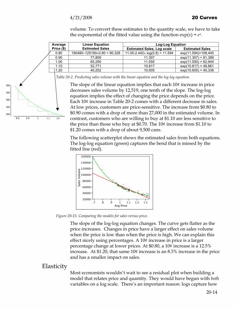
volume. To convert these estimates to the quantity scale, we have to take the exponential of the fitted value using the function exp(x) = ex.

Log-Log Equation Average Price ($)

Linear Equation Estimated Sales Estimated Sales, Log scale Estimated Sales

0.80 190480–125190×0.80 = 90,328 11.05-2.442× log(0.8) = 11.594 exp(11.594)=108,445 0.90 77,809 11.307 exp(11.307) = 81,389 1.00 65,290 11.050 exp(11.050) = 62,944 1.10 52,771 10.817 exp(10.817) = 49,861 1.20 40,252 10.605 exp(10.605) = 40,336

Table 20-2. Predicting sales volume with the linear equation and the log-log equation.

The slope of the linear equation implies that each 10¢ increase in price decreases sales volume by 12,519, one tenth of the slope. The log-log equation implies the effect of changing the price depends on the price. Each 10¢ increase in Table 20-2 comes with a different decrease in sales. At low prices, customers are price-sensitive. The increase from $0.80 to $0.90 comes with a drop of more than 27,000 in the estimated volume. In contrast, customers who are willing to buy at $1.10 are less sensitive to the price than those who buy at $0.70. The 10¢ increase from $1.10 to $1.20 comes with a drop of about 9,500 cans.

The following scatterplot shows the estimated sales from both equations. The log-log equation (green) captures the bend that is missed by the fitted line (red).

20000

40000

60000

80000

100000

120000

140000

160000

Sale

s Vo

lum

e

.7 .8 .9 1 1.1 1.2 1.3Avg Price

Figure 20-15. Comparing the models for sales versus price.

The slope of the log-log equation changes. The curve gets flatter as the price increases. Changes in price have a larger effect on sales volume when the price is low than when the price is high. We can explain this effect nicely using percentages. A 10¢ increase in price is a larger percentage change at lower prices. At $0.80, a 10¢ increase is a 12.5% increase. At $1.20, that same 10¢ increase is an 8.3% increase in the price and has a smaller impact on sales.

Elasticity Most economists wouldn’t wait to see a residual plot when building a model that relates price and quantity. They would have begun with both variables on a log scale. There’s an important reason: logs capture how

4/21/2008 20 Curves

20-15

percentage changes relate price and quantity. Logs change how we think about variation. Variation on a log scale amounts to variation in percentage differences.

The slope in an equation that transforms both x and y using logs is known as the elasticity of y with respect to x. The elasticity describes how small percentage changes in x are associated with percentage changes in y (see Under the Hood: Logs and Percentage Change). In the pet food example, the slope in the log-log model b1 = -2.44 tells us that, on average, a 1% increase in price brings a 2.44% decrease in sales. The intercept in a log-log model is important for calculating

€

ˆ y , but not very interpretable substantively.

What should we tell the retailer? On average, when we compare sales in weeks with prices that differ by 1%, the quantity sold during weeks with the lower price is 2.44% higher than during weeks at the higher price. These cans usually sell for about $1, with typical sales around 60,000 cans per week. If the retailer raises the price by 5% to $1.05, then we’d expect sales volume to fall by 5 × -2.44% = -12.2%. That’s about 0.122 × 60,000 = 7,320 fewer cans, but each of those that do sell bring in $0.05 more. We can find the best price by using the elasticity in a formula that includes the cost to the grocery. If the store spends $0.60 to stock and sell each can, then the price that maximizes profits is (see Under the Hood: Optimal Pricing)

€

Optimal price =cost × elasticity

elasticity +1

=0.60 −2.442( )−2.442 + 1

= $1.016

Most of the time, the retailer has been charging about $1 per can. At $1.02, estimated sales are 60,551; each sale earns $0.52 and profits are $25,189. At the much lower price offered in the discount weeks, the estimated sales are almost double, 108,445 at $0.80 (Table 20-2). At $0.20 profit per can, however, that only nets $21,689. Those big sales might have moved a lot of inventory, but they sacrificed profits.

Example 20.1 Optimal Pricing

Motivation state the question

How much should a convenience store charge for a half-gallon of orange juice? Economics tells us that if orange juice costs c dollars per carton and γ is the elasticity of sales with respect to price, then the optimal price to charge is c γ/(1+γ). For this store, each half-gallon of orange juice costs c = $1 to purchase and stock. All we need to find the best price is the elasticity. We can estimate the elasticity from a regression of the log of sales on the log of price.

elasticity Relates % change in x to % change in y; slope is a log-log regression equation.

tip

4/21/2008 20 Curves

20-16

Method describe the data and select an approach

The explanatory variable will be the price charged per half-gallon, and the response will be the sales volume. Both are transformed using logs. The slope in this equation will estimate the elasticity of sales with respect to price.

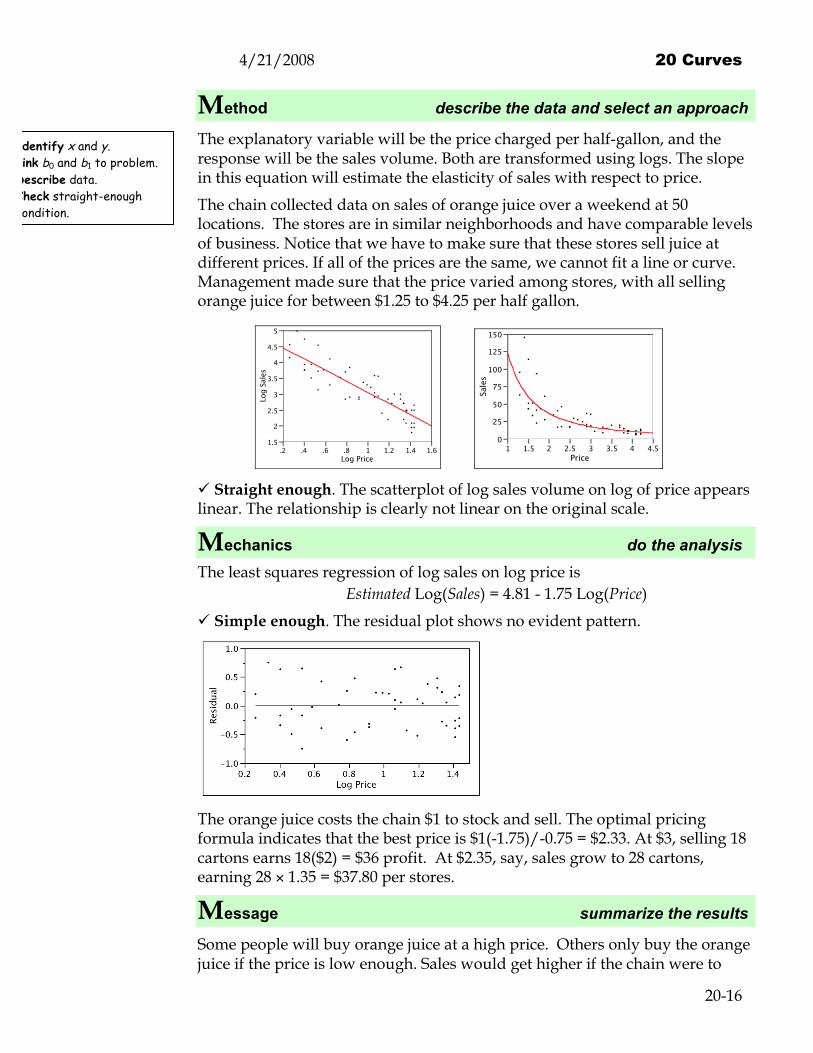
The chain collected data on sales of orange juice over a weekend at 50 locations. The stores are in similar neighborhoods and have comparable levels of business. Notice that we have to make sure that these stores sell juice at different prices. If all of the prices are the same, we cannot fit a line or curve. Management made sure that the price varied among stores, with all selling orange juice for between $1.25 to $4.25 per half gallon.

1.5

2

2.5

3

3.5

4

4.5

5

Log

Sale

s

.2 .4 .6 .8 1 1.2 1.4 1.6Log Price

0

25

50

75

100

125

150

Sales

1 1.5 2 2.5 3 3.5 4 4.5Price

Straight enough. The scatterplot of log sales volume on log of price appears linear. The relationship is clearly not linear on the original scale.

Mechanics do the analysis The least squares regression of log sales on log price is

Estimated Log(Sales) = 4.81 - 1.75 Log(Price)

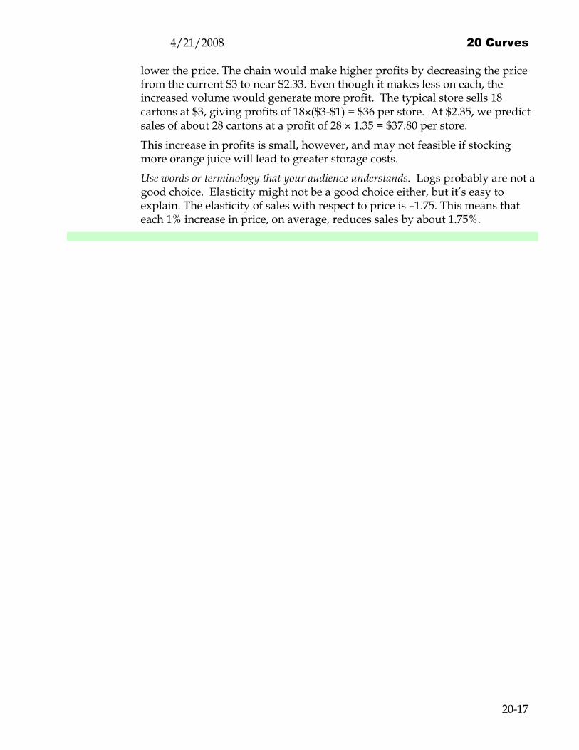
Simple enough. The residual plot shows no evident pattern.

The orange juice costs the chain $1 to stock and sell. The optimal pricing formula indicates that the best price is $1(-1.75)/-0.75 = $2.33. At $3, selling 18 cartons earns 18($2) = $36 profit. At $2.35, say, sales grow to 28 cartons, earning 28 × 1.35 = $37.80 per stores.

Message summarize the results

Some people will buy orange juice at a high price. Others only buy the orange juice if the price is low enough. Sales would get higher if the chain were to

Identify x and y. Link b0 and b1 to problem. Describe data. Check straight-enough condition.

4/21/2008 20 Curves

20-17

lower the price. The chain would make higher profits by decreasing the price from the current $3 to near $2.33. Even though it makes less on each, the increased volume would generate more profit. The typical store sells 18 cartons at $3, giving profits of 18×($3-$1) = $36 per store. At $2.35, we predict sales of about 28 cartons at a profit of 28 × 1.35 = $37.80 per store.

This increase in profits is small, however, and may not feasible if stocking more orange juice will lead to greater storage costs.

Use words or terminology that your audience understands. Logs probably are not a good choice. Elasticity might not be a good choice either, but it’s easy to explain. The elasticity of sales with respect to price is –1.75. This means that each 1% increase in price, on average, reduces sales by about 1.75%.

4/21/2008 20 Curves

20-18

Summary Regression equations use transformations of the original variables to describe patterns that curve. Equations with reciprocals and logs are useful in many business applications and are readily interpretable. Nonlinear equations that use these transformations allow the slope to change, implying that the effect of the relationship between the explanatory variable on the response depends on the value of the explanatory variable. The slope in a regression model that uses logs of both the response and explanatory variable is the elasticity of the response with respect to price.

Index elasticity, 20-15, 20-21 transformation, 20-6

Best Practices • Check that a line summarizes the relationship between the

explanatory variable and response both visually and substantively. Lines are common and simple, but not always the best summary of dependence. A linear pattern implies that changes in the explanatory variable have the same effect on the response, regardless of the size of the predictor variable. Often, particularly in economic problems, the effect of the predictor depends on its size.

• Stick to models you can understand and interpret. Reciprocals are a natural transformation if your data is already a ratio. Logs are harder to motivate, but are so common in economic modeling, such as in demand curves, to be worth considering.

• Interpret the slope carefully. Slopes in models that use logs or other transformations mean different things than slopes in a linear model. In particular, the slope in a log-log model is an elasticity, telling you how % changes in x are associated with % changes in y.

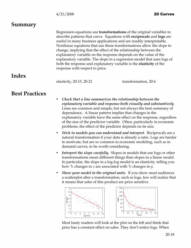
• Show your model in the original units. If you show most audiences a scatterplot after a transformation, such as logs, few will realize that it means that sales of this product are price sensitive.

1.5

2

2.5

3

3.5

4

4.5

5

Log

Sale

s

.2 .4 .6 .8 1 1.2 1.4 1.6Log Price

0

25

50

75

100

125

150

Sales

1 1.5 2 2.5 3 3.5 4 4.5Price

Most hasty readers will look at the plot on the left and think that price has a constant effect on sales. They don’t notice logs. When

4/21/2008 20 Curves

20-19

shown on the original scales, it’s immediate that the effect of price increases diminishes at higher prices.

Pitfalls • Thinking that regression only fits straight lines. It’s common to

think that regression equations only fit straight lines. That’s because, once we use the right transformation, we do fit straight lines. To see the curvature, you have to return to the original scales.

• Missing the bend. You won’t discover the curvature unless you look for it. Examine the residuals, and pay special attention to the most extreme residuals because they may have something to add to the story told by the linear model. It’s often easier to see deviations from a straight line in the residual plot than in the scatterplot of the original data.

• Modeling data that you don’t understand. One of the keys to finding curvature is understanding the context of your data. It’s more natural, for example, to think of the effect of price on quantity in percentage terms. Plots of marginal revenue or costs are typically nonlinear.

• Forgetting lurking variables. Another consequence of not understanding the data is forgetting that these equations describe association, not causation. It’s easy to get caught up in figuring out the right transformation and forget other factors. Unless we can rule out other factors, we don’t know that changing the price of a product caused the quantity sold to change. Perhaps every time in the past when the retailer raised prices, so did the competition.. Consumers always saw the same difference in prices. Unless that matching continues the next time the price changes, the response may be very different.

• Comparing r2 in models with different responses. You can only compare r2 between models with the same response. For instance, it makes no sense to compare the proportion of variation in the log of quantity to the proportion of variation in the quantity itself.

• Using too many transformations. Equations like this one used by NASA to study the space shuttle (Chapter 1) don’t always infuse audiences with confidence that you know what you’re doing.

€

p =0.0195 L /d( )0.45 d( )ρF0.27 V −V *( )

2 / 3

ST1/ 4ρT

1/ 6

Unless you can make sense of your model in terms that others appreciate, you’re not going to find curves that useful.

4/21/2008 20 Curves

20-20

Under the Hood: Logs and Percentage Changes The slope in a linear equation indicates how the estimate of y changes when x grows by 1. Denote the estimate of y at x by

€

ˆ y (x) = b0+b1 x, and the estimate of y at x+1 by

€

ˆ y (x+1) = b0+b1 (x+1). The slope is the difference between these estimates:

€

ˆ y (x+1) –

€

ˆ y (x) = (b0 + b1 (x + 1)) – (b0 + b1 x) = b1

To interpret a log-log equation, think in terms of percentages. Instead of looking for what to expect when x grows by 1, think in terms what happens when x grows by 1%. The predicted value for the log of y in the log-log equation at x is

€

log ˆ y (x) = b0 + b1 log x

Rather than increase x by adding 1, multiply x by 1.01 to increase it by 1%. If x increases by 1%, the predicted value becomes

€

log ˆ y (1.01x) = b0 + b1 log(1.01x)= b0 + b1 log x + b1 log 1.01= log ˆ y (x) + b1 log 1.01≈ log ˆ y (x) + 0.01b1

The last step uses a simple but useful approximation: log (1 + little bit) ≈ little bit

This approximation is accurate so long the little bit is less than 0.10. In this example, the approximation means log(1.01) = log(1 + 0.01) ≈ 0.01. If we rearrange the previous equation and remember that

log a – log b = log (a/b),

then the estimated change that comes with a 1% increase in x is

€

0.01b1 = log ˆ y (1.01x) − log ˆ y (x)

= logˆ y (1.01x)

ˆ y (x)

= logˆ y (x) + ˆ y (1.01x) − ˆ y (x)( )

ˆ y (x)

= log 1+ˆ y (1.01x) − ˆ y (x)

ˆ y (x)

≈ˆ y (1.01x) − ˆ y (x)

ˆ y (x)

Change x by 1% and the fitted value changes by

€

b1 ≈100ˆ y (1.01x) − ˆ y (x)

ˆ y (x)= Percentage change in ˆ y

The slope b1 in a log-log model tells you how percentage changes in x (up to about ±10%) translate into percentage changes in y.

little bit

4/21/2008 20 Curves

20-21

Under the Hood: Optimal Pricing Choosing the price that earns the most profit requires a bit of economic analysis. In the so-called monopolist situation, economics describes how the quantity sold Q depends on the price p according to an equation like this one, Q(p) = m pγ. The theory constrains the exponent γ < -1. The symbol m stands for a constant that depends, for example, on whether we’re measuring sales in cans or cases. The exponent γ is the elasticity of the quantity sold with respect to price.

We don’t want to maximize sales – it’s profits that matter. Suppose each item costs the seller c dollars. Then the profit at the selling price p is

Profit(p) = Q(p) (p – c)

Calculus shows that the price that maximizes the profit is

p* = c γ/(1 + γ)

For example, if each item costs c = $1 and the elasticity γ = -2, then the optimal price is c γ/(1 + γ) = $1 × -2/(1-2) = $2. If customers are more price sensitive and γ = -3, the optimal price is $1.50. As the elasticity approaches –1, the optimal price soars (tempting governments to regulate prices).

About the Data A former Wharton MBA student worked in the auto industry and provided the data in this chapter that describe characteristics of cars. The mileage data is the standard EPA estimate for urban driving. Highway mileage produces similar results.

The pricing data also comes from an MBA student who worked with a retailer during her summer internship. We modified the data slightly to protect the source of the data.

Software Hints There are two general approaches to fitting curves. In some cases, you can add the curve itself to a scatterplot of the actual data. Rather than transform, say, both X and Y to a log scale, you can add the curve that summarizes the fit of log Y on log X directly to the scatterplot of Y on X. (For example, see Figure 20-8.) However, most software instead forces you to transform the data. That is, you need to first build two new columns, one holding the logs of Y and the other holding logs of X. Then, you proceed to build a scatterplot of these two transformed columns. Fitting the line in the scatterplot of log Y on log X gives the equation for the curve in the original units.

Excel To help you decide if a transformation is necessary, start with the scatterplot of Y on X. With the chart selected, the menu sequence

4/21/2008 20 Curves

20-22

Chart > Add Trendline… allows you to fit several curves to your data (as well as a line). Try several and decide which fit provides the best summary of the data.

If you believe that the association between Y and X bends, use built-in functions to compute columns of transformed data (for example, make a column that is equal to the LOG or reciprocal of another). Then follow the methods in the prior chapter to fit a line to the transformed data.

Minitab If the scatterplot of Y on X shows a bending pattern, use the calculator (menu sequence Calc > Calculator…) to construct columns of transformed data (i.e., build new variables such as 1/X or log Y). Then follow the methods in the prior chapter to fit a line to the transformed data.

JMP The menu sequence

Analyze > Fit Y by X opens the dialog used to construct a scatterplot. Fill in variables for the response and explanatory variable, then click OK. In the window that shows the scatterplot, click on the red triangle above the scatterplot (near the words “Bivariate Fit of …”). In the pop-up menu, choose the item Fit Special to fit curves to the shown data. Select a transformation for Y or X and JMP will estimate the chosen curve by least squares, add the fit to the scatterplot, and add a summary of the equation to the output below the plot. If you would like to see the associated linear fit to the transformed data, you’ll need to use the JMP formula calculator to build new columns (new variables). For example, right-clicking in the header of an empty column in your spreadsheet allows you to define the column using a formula such as Log(X).